Controlling spatiotemporal chaos via small external forces

The spatiotemporal chaos in the system described by a one-dimensional nonlinear drift-wave equation is controlled by directly adding a periodic force with appropriately chosen frequencies. By dividing the solution of the system into a carrier steady wave and its perturbation, we find that the controlling mechanism can be explained by a slaving principle. The critical controlling time for a perturbation mode increases exponentially with its wave number.

PACS numbers:05.45+b, 52.35.Kt, 52.35.-g

I Introduction

Spatiotemporal chaos(STC) can appear in a large variety of systems such as hydrodynamic systems, plasma devices, laser systems, chemical reactions, Josephson junction arrays and biological systems. Because of the potential applications, controlling STC in these systems has been given much attention by scientists and technologists in recently years[1]-[12]. Generally speaking, there are two kinds of methods to control STC: the feedback control[1]-[8] and the nonfeedback one[9]-[12]. For the former one, it needs a fast responding feedback system that produces an external signal in response to the system’s dynamics. On the contrary, for the later one, the form and the amplitude of the external control signal can be adjusted numerically or experimentally by directly observing the response of the system to the applied signal. The advantages and disadvantages of the two kinds of methods are: for the feedback one, the reference state is always an unstable trajectory locating in the chaotic attractors, the controlling input is very small if the system can be well controlled, in this way, however, one must know some prior knowledge of the system before controlling; In contrast, for the nonfeedback one, it does not need any prior knowledge of the system, it is very easy in practice, and particularly convenient for experimentalist, but the target states are not the unstable periodic orbits of the chaotic attractors, hence, the controlling input does not vanish when the system is under control.

In this letter, we will give an example of controlling STC by adding a small external force on a system and discuss the mechanism. In fact, the methods of adding a pre-determined driving force or modifying an accessible parameter in a pre-determined way on the system to control chaos might be firstly used by Alekseev and Loskutov[13], who studied how to control a chaotic model of a water ecosystem by small periodic perturbations. After Alekseev and Loskutov, Lima and Pettini[14] successfully used the parametric perturbation method to eliminate chaos in Duffing-Holmes oscillator. Some experimental works about the method have been done by Azevedo[15],Fronzoni[16], Ding[17] and Ciofini[18]. Moreover, Braiman and Goldhirsch[19] directly added a weak external periodic force to Josephson junction system to suppress chaos even in nonresonant circumstance. Recently, the method has been intensively and extensively used to control chaos not only for nonautonomous systems but also for autonomous systems and iterated maps[20]. However, within our knowledge, the method has not ever been used to control STC. This letter will give the first example to use the method to control STC in a partial differential equation systems, and find for the first time that the mechanism can be explained by the slaving principle.

The letter is organized as follows. First, we will briefly introduce the driven-damped nonlinear drift-wave equation which we used as the model equation. Then, the control method and the numerical simulation results will be given. Next, we will analyze the controlling mechanism. Finally, a discussion and conclusion will be given.

II Model

The model we used in this letter is a one-dimensional nonlinear drift-wave equation driven by a sinusoidal wave. It reads[21]

$$\frac{\partial\phi}{\partial t}+a\frac{\partial^{3}\phi}{\partial t\partial x^{2}}+c\frac{\partial\phi}{\partial x}+f\phi\frac{\partial\phi}{\partial x}=-\gamma\phi-\epsilon\sin(x-\Omega t),$$ (1)

where the $2\pi$-periodic boundary condition,$\phi(x+2\pi,t)=\phi(x,t)$, is applied. In this study, we fix the parameters $a=-0.2871$, $\gamma=0.1$, $c=1.0$ and $f=-6.0$ , only the forcing strength $\epsilon$ and phase speed $\Omega$ of the sinucoidal wave are the control parameters. Without the dissipation and driving terms($\gamma=0$, $\epsilon=0$), Eq. (1) describes the nonlinear drift-wave in magnetized plasmas [22]. After introducing the driving and dissipation terms, the competition among dispersion, dissipation, driving and nonlinearity makes the system display rich dynamic phenomena[21][23].

In plasma physics, an integral quantity $E(t)$, which is well known as the ”energy” of the system,

$$E(t)=\frac{1}{2\pi}\int_{0}^{2\pi}\frac{1}{2}[\phi^{2}(x,t)-a(\frac{\partial\phi}{\partial z})^{2}]dz,$$ (2)

is conveniently used to monitor the dynamics of the system. $E(t)$ is a positive constant at $\epsilon=\gamma=0$ and monotonously decreases to zero by the dissipation if $\epsilon=0$ and $\gamma>0$.

In the present paper, we focus on STC states. On the parameter plane $\epsilon-\Omega$, the dynamic behavior of the system has been extensively studied by one of us(He)[21, 23]. According to Fig. 6(b) in Ref. [23], one can find that in certain regions of $\Omega$, when the driving $\epsilon$ is strong enough the system displays a STC state. It is necessary to point out that so called space-time chaos is an ambiguous terminology. There is evidence to show that the spatial incoherence may be caused by different physical effects. In previous work[24], Hu and He reported an example of controlling one type of STC states by feedback method, its erratic spatial behavior is due to the overlapping of the regimes of the Hopf instability of different modes. In the present work, we will focus our attention on a STC state, e.g. at $\epsilon=0.22,\Omega=0.65$, the transition to STC is caused by a crisis[23].

III Methods and numerical simulation results

For controlling STC in the system, we directly add a small temporally periodic signal on the right hand side of Eq. (1). Thus Eq. (1) is changed to

$$\frac{\partial\phi}{\partial t}+a\frac{\partial^{3}\phi}{\partial t\partial x^{2}}+c\frac{\partial\phi}{\partial x}+f\phi\frac{\partial\phi}{\partial x}=-\gamma\phi-\epsilon\sin(x-\Omega t)+\eta\cos(\omega t),$$ (3)

where $\eta$ and $\omega$ are the control parameters.

The pseudospectral method[25] is used to simulate Eq. (3). In the numerical simulation, we divide the space into 128 points. 256 and 512 points have also been used, the results do not show qualitative difference. Therefore, the 128 points are used in our work.

In order to find suitable $\eta$ and $\omega$ to control STC, we first calculate the power spectrum of $\phi(x_{0},t)$, denoted by $S(\omega)$, at a fixed point $x=x_{0}$ in space. From the power spectrum $S(\omega)$ one can find the characteristic frequency region of the chaotic attractor. For example, Fig. 1(a) shows the spectrum of the STC state to be controlled, from this figure one can see that except for the frequency of driving wave($\Omega=0.65$), there are many peaks in the region $\omega\in[0.2,0.9]$. Our experience shows that the appropriate $\omega$ for a successful control should be chosen in this region. Now, fix an $\omega$ in this region, one can try to find a suitable $\eta$. We find some windows in $\omega-\eta$ plane, with which parameters the turbulent motion of the STC state can be successfully suppressed. The results are given in Fig. 2, in which the circles stand for the suitable parameter points for controlling STC in system (1), while the crosses indicate the parameter points at which the turbulence are failed to be controlled. In the following, we choose $\omega=0.756$ and $\eta=0.1$ as an example. To compare the dynamic behavior of the system before and after the control, the power spectrum, energy and spatiotemporal patterns are calculated. Figure 1(b) shows the power spectrum $S(\omega)$ at a fixed space point($x=\pi$) after the control. In contrast to the wide noisy spectrum in Fig. 1(a), here only a few lines are left. In Fig. 3, We give the time series of the energy $E(t)$, one can see it is chaotic before control, which becomes harmonic oscillations after a while when the control signal is added. The spatiotemporal patterns of the system before and after control are shown in Fig. 4(a) and Fig. 4(b), respectively, obviously the turbulence is strongly suppressed .

IV Mechanism and Scaling behavior

To analyze the mechanism of the control method introduced above, firstly, let us observe the solution of Eq. (3) in the frame of the driving wave. By setting $z=x-\Omega t$ and $\tau=t$ , Eq. (3) can be rewritten as

$$\frac{\partial}{\partial\tau}(1+a\frac{\partial^{2}}{\partial z^{2}})\phi=\Omega\frac{\partial}{\partial z}(1+a\frac{\partial^{2}}{\partial z^{2}})\phi-c\frac{\partial\phi}{\partial z}-f\phi\frac{\partial\phi}{\partial z}-\gamma\phi-\epsilon\sin z+\eta\cos(\omega\tau).$$ (4)

Then, we divide a solution of Eq. (3) into a carrier steady wave $\phi_{0}(z)$, and it’s perturbation $\delta\phi(z,t)$, i.e.,

$$\phi(z,t)=\phi_{0}(z)+\delta\phi(z,t).$$ (5)

Here $\phi_{0}$ satisfies the steady equation $\partial\phi_{0}/\partial\tau=0$, i.e.,

$$\Omega\frac{\partial}{\partial z}(1+a\frac{\partial^{2}}{\partial z^{2}})\phi_{0}-c\frac{\partial\phi_{0}}{\partial z}-f\phi_{0}\frac{\partial\phi_{0}}{\partial z}-\gamma\phi_{0}-\epsilon\sin z=0.$$ (6)

Insert Eq. (5) into Eq. (4), and using Eq. (6), one has

$$\frac{\partial}{\partial\tau}(1+a\frac{\partial^{2}}{\partial z^{2}})\delta\phi = \Omega\frac{\partial}{\partial z}(1+a\frac{\partial^{2}}{\partial z^{2}})\delta\phi-c\frac{\partial\delta\phi}{\partial z}-f\phi_{0}\frac{\partial\delta\phi}{\partial z}-f\delta\phi\frac{\partial\phi_{0}}{\partial z}-f\delta\phi\frac{\partial\delta\phi}{\partial z}$$ (8)

$$-\gamma\delta\phi+\eta\cos(\omega\tau).$$

By making the Fourier transformation of $\phi_{0}(z)$ and $\delta\phi(z,t)$ as

$$\left\{\begin{array}[]{l}\phi_{0}(z)=A_{0}+lim_{N\rightarrow\infty}\sum_{k=1}^{N}A_{k}\cos(kz+\theta_{k}),\\ \delta\phi(z,t)=b_{0}(t)+lim_{N\rightarrow\infty}\sum_{k=1}^{N}b_{k}(t)\cos(kz+\alpha_{k}(t)),\end{array}\right.$$ (9)

Eq. (6) is transformed to a set of infinite algebraic equations, and Eq. (8) a set of infinite ordinary differential equations

$$\left\{\begin{array}[]{l}\frac{db_{0}}{dt}=-\gamma b_{0}+\eta\cos(\omega t),\\ \frac{db_{k}}{dt}=N_{k}(t)+fkb_{0}A_{k}\sin(\theta_{k}-\alpha_{k})/(1-ak^{2}),\\ \frac{d\alpha_{k}}{dt}=M_{k}(t)-\frac{fk(A_{0}+b_{0})}{(1-ak^{2})}-\frac{fkb_{0}A_{k}\cos(\theta_{k}-\alpha_{k})}{(1-ak^{2})b_{k}},\end{array}\right.$$ (10)

where

$$N_{k}(t)= - \frac{\gamma b_{k}}{1-ak^{2}}+\frac{fk}{2(1-ak^{2})}$$ (11)

$$\times \{\sum_{l+l^{\prime}=k}[A_{l}b_{l^{\prime}}\sin(\theta_{l}+\alpha_{l^{\prime}}-\alpha_{k})+\frac{1}{2}b_{l}b_{l^{\prime}}\sin(\alpha_{l}+\alpha_{l^{\prime}}-\alpha_{k})]$$ (12)

$$+ \sum_{l-l^{\prime}=k}[A_{l}b_{l^{\prime}}\sin(\theta_{l}-\alpha_{l^{\prime}}-\alpha_{k})+\frac{1}{2}b_{l}b_{l^{\prime}}\sin(\alpha_{l}-\alpha_{l^{\prime}}-\alpha_{k})]$$ (13)

$$+ \sum_{l^{\prime}-l=k}[A_{l}b_{l^{\prime}}\sin(-\theta_{l}+\alpha_{l^{\prime}}-\alpha_{k})+\frac{1}{2}b_{l}b_{l^{\prime}}\sin(-\alpha_{l}+\alpha_{l^{\prime}}-\alpha_{k})]\},$$ (14)

$$M_{k}(t)= - k(\frac{c}{1-ak^{2}}-\Omega)-\frac{kf}{2(1-ak^{2})b_{k}}$$ (15)

$$\times \{\sum_{l+l^{\prime}=k}[A_{l}b_{l^{\prime}}\cos(\theta_{l}+\alpha_{l^{\prime}}-\alpha_{k})+\frac{1}{2}b_{l}b_{l^{\prime}}\cos(\alpha_{l}+\alpha_{l^{\prime}}-\alpha_{k})]$$ (16)

$$+ \sum_{l-l^{\prime}=k}[A_{l}b_{l^{\prime}}\cos(\theta_{l}-\alpha_{l^{\prime}}-\alpha_{k})+\frac{1}{2}b_{l}b_{l^{\prime}}\cos(\alpha_{l}-\alpha_{l^{\prime}}-\alpha_{k})]$$ (17)

$$+ \sum_{l^{\prime}-l=k}[A_{l}b_{l^{\prime}}\cos(-\theta_{l}+\alpha_{l^{\prime}}-\alpha_{k})+\frac{1}{2}b_{l}b_{l^{\prime}}\cos(-\alpha_{l}+\alpha_{l^{\prime}}-\alpha_{k})]\},(k=1,2,\dots,N).$$ (18)

In numerical simulations, the mode equations for ${A_{k},\theta_{k}}$ and ${b_{k},\alpha_{k}}$ can be solved simultaneously with truncation. The proper $N$ should satisfy the condition that the modes $k>N$ give negligible contributions to the actual solution of the equation[24]. For the present parameters we use $N=13$, i.e., the 27-dimensional ordinary differential equations will be solved. With these mode equations one can obtain qualitatively the same results as the direct simulating Eq. (3).

Now let us analyze the numerical results of the solution of Eqs. (10). From the time evolution curves of $b_{k}$, one can see that, for every mode $k$, there exists a turning point $\tau_{k}^{*}$, before which $b_{k}$ shows chaotic motion with larger amplitude, while after which it becomes a quasi-periodic vibration with much smaller amplitude. As an example, Fig. 5(a) depicts the time evolution of $b_{3}$ and $b_{11}$ in the beginning 50 time units after the control signal is added and another 50 time units when they behave quasi-periodically. In order to determine $\tau_{k}^{*}$, let us calculate the relative average amplitude value of each mode

$$r_{k}(t)=(b_{k}^{*}(t)-\bar{b_{k}})/\bar{b_{k}},$$ (19)

where $\bar{b}_{k}$ is the time average value of $b_{k}$ in the quasi-periodic states, $b_{k}^{*}$ is the points only on the Poincaré section[26]. As an example, the results of $r_{8}(t)$,$r_{10}(t)$ and $r_{12}(t)$ are shown in Fig. 5(b), one can see that, after adding the periodic control signal, $r_{k}(t)$ starts to decrease exponentially, but they never tend to zero. After a certain time point, the oscillation level of each $r_{k}$ no longer decrease.

Next, we will study the dependence of the critical point $\tau_{k}^{*}$ on the mode number $k$. In the decreasing phase of $r_{k}$, its maxima decreasing linearly in the logarithmic diagram, while in the quasiperiodic phase, the maxima of $b_{k}$ are about a constant. The intersection point of the two straight lines gives $\tau_{k}^{*}$. In Fig. 5(c), we plot $\tau_{k}^{*}$ as a function of mode number $k$ in the semilogarithmic plane, the points can be well fitted by a straight line. Consequently we obtain a scaling law

$$\tau_{k}^{*}\propto e^{\beta k},$$ (20)

here by the least square method we get $\beta=0.1169$. When amplitude $b_{k}$’s transit to the quasi-periodic phase, the mode phase ,$\alpha_{k}$, of the originally chaotic mode also become very quiescent. We can also determine the turning points $\tau_{k}^{*}$ from the evolution of $\alpha_{k}$, the same scaling law as Eq. (20) is obtained, with $\beta=0.1158$.

From these results we conclude that, by using our time-periodic signal to control a STC state, the modes$\{b_{k},\alpha_{k}\}$ will be controlled one by one from the smallest wave number $k$ to the highest one. The critical time for a mode to be controlled increases exponentially with the wave number $k$. This phenomenon can be understood by the slaving principle in synergetics[27]. From the first equation of Eqs. (10), one can see that, in fact, the external force is added on the mode $k=0$, the evolution of $b_{0}$ is uniquely determined by the applied control signal and the dissipation rate $\gamma$. Its motion does not influenced by the other $k\neq 0$ modes. The motion of $b_{0}$ is adjusted to periodic one very quickly after the control signal is added. Then the other modes $k\neq 0$ are slaved by $b_{0}$. This fact can be seen from Eqs.(10) for $k\neq 0$. In both equations for $b_{k}$ and $\alpha_{k}$, there is a term depending on $b_{0}$, which is the contribution of the mode-mode couplings between $b_{0}$,$\{A_{k},\theta_{k}\}$ and $\{b_{k},\alpha_{k}\}$. Through these terms $b_{0}$ plays the slaving role. Meanwhile, since the modes of the steady wave $\phi_{0}(z)$, $\{A_{k},\theta_{k}\}$ are constants in the frame of $\{z,\tau\}$. the modes $\{b_{k},\alpha_{k}\}$ also play a significant role in the solving process. Moreover, the numerical results tell us that $b_{0}$ is a slowly relaxing variable and the other modes are fast ones in the beginning stage when the control signal is just added. Thus, $b_{0}$ plays an important role as an order parameter in the system, and it is affected by the control force. When the control signal is added, $b_{1}$ and $\alpha_{1}$ are immediately slaved by $b_{0}$. Since the effect of $b_{0}$ on $\{b_{k},\alpha_{k}\}$ is through $\{A_{k},\theta_{k}\}$ and $A_{k}$ decrease with $k\rightarrow\infty$ , the slaving intensity is not unform for different modes. From Eqs. (10), one can see that the smaller the mode $k$, the higher the slaving intensity it has. So the mode $k=1$ can be controlled firstly. Then, it starts to slave the modes $k=2,3,...$, until all the modes are tamed. In the whole process, the system changes from an extremely disordered(a STC state) into an ordered one by the self-organization principle.

V Conclusion and discussion

In conclusion, we have successfully suppressed very turbulent STC states by directly adding a temporally periodic force on the system. The appropriate input frequency can be chosen by analyzing the spectrum of the turbulence. In contrast to the feedback method for which one needs the knowledge of the target state, the present method is easy to be realized in practical experiments. The controlling mechanism is studied by investigating the evolution of perturbation wave to the carrier steady wave. We find that the perturbation modes are controlled one-by-one from long to short wave length by a slaving principle, and the critical controlling time for the mode increases exponentially with its wave number $k$. Since the slaving effect is very important in nonlinear science, these results may be interested in by scientists and engineers. The schemes of how to select the controlling frequency may also be helpful for the experimentalists.

ACKNOWLEDGMENTS

The first author(Wu) would like to thank Drs. Baisong Xie and Luqun Zhou for useful discussions. This work is supported by the National Natural Science Foundation of China under grant No. 19675006, No. 19835020 and the Research Funds for the Doctoral Program of Higher Education under the grant No. 98002713.

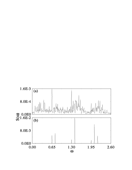
FIG. 1.: Power spectrum of potential at fixed $z$($z=\pi$) before(a) and after(b) control. The time interval,$\Delta t$, between consecutive samples is $0.5$, The 1024 points are used to do the FFT, the total sample points are $4096$.

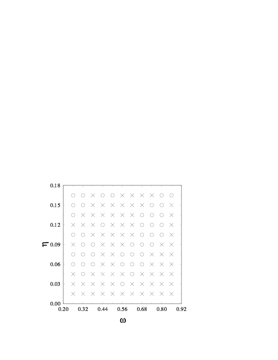
FIG. 2.: Global view of control parameters on the plane $\omega-\eta$. Points $\circ$ and $\times$ stand for the suitable and unsuitable parameter points for controlling STC in system (1),respectively.

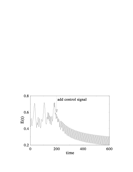
FIG. 3.: The energy E(t) as a function of time before and after control.                          

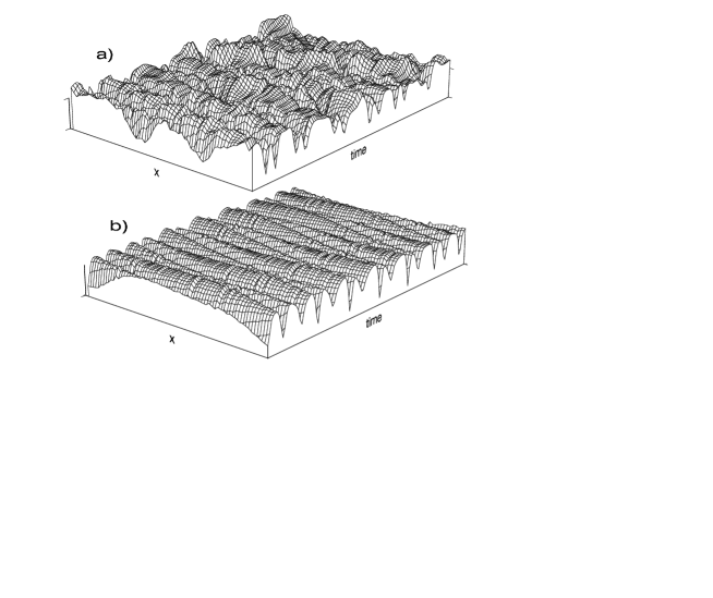
FIG. 4.: Spatiotemporal patterns of $\phi(z,t)$ before(a) and after(b) control.                          

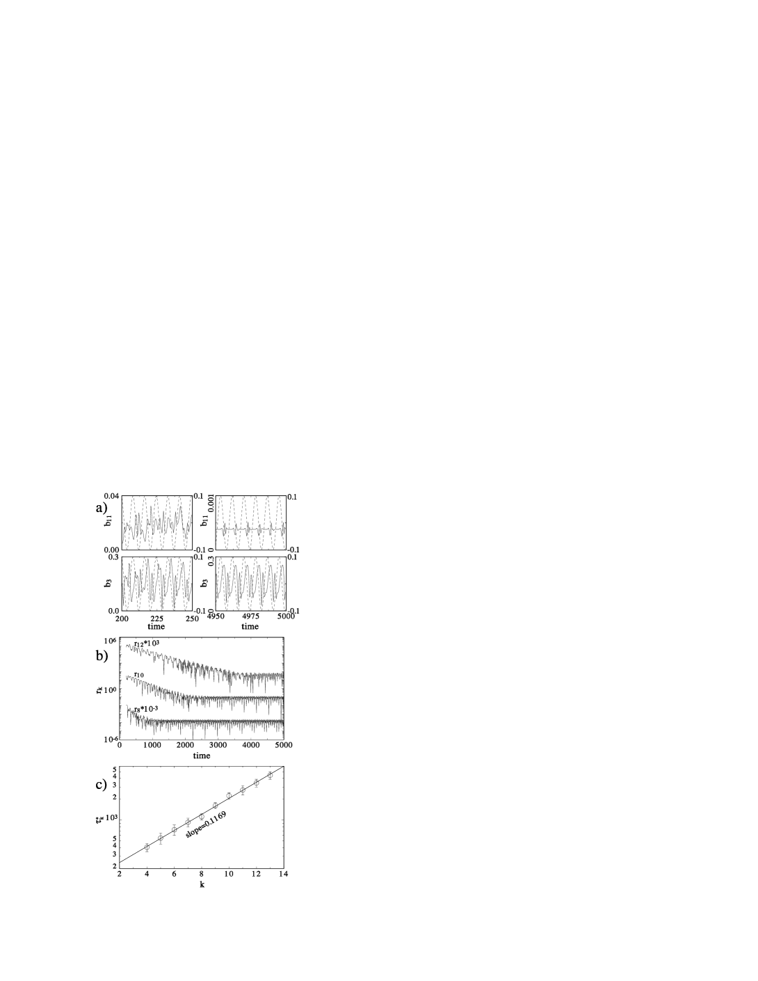
FIG. 5.: (a) The evolution of the amplitudes, $b_{k}(t)(k=3,11)$, for the perturbation wave, the dashed lines scaled by the right axises indicate the external force. (b) The evolution of $r_{k}(k=8,10,12)$. (c) The scaling law of $\tau_{k}^{*}$.

REFERENCES

- [1] G. Hu and Z. Qu, Phys. Rev. Lett. 72, 68 (1994).
- [2] D. Auerbach, Phys. Rev. Lett. 72, 1184 (1994).
- [3] F. Qin, E.E. Wolf, and H.-C. Chang, Phys. Rev. Lett. 72, 1459 (1994).
- [4] G. Hu, Z. Qu, and Kaifen He, Int. J. of Bifurcation and Chaos 5, 901 (1995).
- [5] W. Lu, D. Yu, and R.G. Harrison, Phys. Rev. Lett. 76, 3316 (1996).
- [6] E. Tziperman, H. Scher, S.E. Zebiak, and M.A. Cane, Phys. Rev. Lett. 79, 1034 (1997).
- [7] R.O. Grigoriev, M.C. Cross, and H.G. Schuster, Phys. Rev. Lett. 79, 2795 (1997).
- [8] P. Parmananda and Yu. Jiang, Phys. Lett. A 231, 159 (1997).
- [9] I. Aranson, H. Levine, and L. Tsimring, Phys. Rev. Lett. 72, 2561 (1994).
- [10] Y. Braiman, J.F. Lindner, and W.L. Ditto, Nature(Landon) 378, 465 (1995).
- [11] N. Parekh, S. Parthasarathy, and S. Sinha, Phys. Rev. Lett. 81, 1401 (1998).
- [12] R. Montagne and P. Colet, Int. J. of Bifurcation and chaos 8, 1849 (1998).
- [13] V.V. Alekseev and A.Y. Loskutov, Soviet Phys. Dokl. 32, 1346 (1987).
- [14] R. Lima and M. Pettini, Phys. Rev. A 41, 726 (1989).
- [15] A. Azevedo and S.M. Rezende, Phys. Rev. Lett. 66, 1342 (1991).
- [16] L. Fronzoni, M. Giocondo, and M. Pettini, Phys. Rev. A 43, 6483 (1991).
- [17] W.X. Ding, H.Q. She, W. Huang, and C.X. Yu, Phys. Rev. Lett. 72, 96 (1994).
- [18] M. Ciofini, R. Meucci, and F.T. Arecchi, Phys. Rev. E 52, 94 (1995).
- [19] Y. Braiman and I. Goldhirsch, Phys. Rev. Lett. 66, 2545 (1991).
- [20] D. Cai, A.R. Bishop, N. Gronbech-Jensen, and B.A. Malomed, Phys. Rev. E 49, 1000 (1994); G. Cicogna and L. Fronzoni, Phys. Rev. E 47, 4585 (1993); D. Iracane and P. Bamas Phys. Rev. Lett 67, 3086 (1991); Y.S. Kivshar, F. Rodelsperger, and H. Benner, Phys. Rev. E 49, 319 (1994); Z.L. Qu, G. Hu, G.J. Yang, and G. R. Qin, Phys. Rev. Lett. 74, 1736 (1994); E.F. Stone, Phys. Lett. A 163, 367 (1992); S.T. Vohra, L. Fabiny, and K. Wiesenfeld, Phys. Rev. Lett. 72, 1333 (1994); Y. Liu and J.R.R. Leite, Phys. Lett. A 185, 35 (1994); R.-R. Hsu, H.-T. Su, J.-L. Chern, and C.-C. Chen, Phys. Rev. Lett. 78, 2936 (1997).
- [21] Kaifen He and A. Salat, Plasma Phys. and Controlled Fusion 31, 123 (1989).
- [22] V. Oraevskii, H. Tasso, and H. Wobig, in Proc. 3rd Int. Conf. on Plasma Physics and Controlled Nuclear Fusion Research, Novosibirsk,1968 (IAEA,Vienna,1969) Vol.1, p.167.
- [23] Kaifen He, Phys. Rev. Lett. 80, 696 (1998).
- [24] G. Hu and Kaifen He, Phys. Rev. Lett. 71, 3794 (1993).
- [25] S.A. Orszag, Studies in Applied Mathematics L(4), 293 (1971)
- [26] Here, the Poincaré section is the time at which the control signal has a minimum value.
- [27] H. Haken, Synergetics, An Introduction, 2nd Ed. (Springer-Verlag, Berlin Heidelberg New York, 1978 )