Thermostating by deterministic scattering:
the periodic Lorentz gas

Abstract

We present a novel mechanism for thermalizing a system of particles in equilibrium and nonequilibrium situations, based on specifically modeling energy transfer at the boundaries via a microscopic collision process. We apply our method to the periodic Lorentz gas, where a point particle moves diffusively through an ensemble of hard disks arranged on a triangular lattice. First, collision rules are defined for this system in thermal equilibrium. They determine the velocity of the moving particle such that the system is deterministic, time reversible, and microcanonical. These collision rules can systematically be adapted to the case where one associates arbitrarily many degrees of freedom to the disk, which here acts as a boundary. Subsequently, the system is investigated in nonequilibrium situations by applying an external field. We show that in the limit where the disk is endowed by infinitely many degrees of freedom it acts as a thermal reservoir yielding a well–defined nonequilibrium steady state. The characteristic properties of this state, as obtained from computer simulations, are finally compared to the ones of the so–called Gaussian thermostated driven Lorentz gas.

PACS numbers: 05.20.-y, 05.45.+b, 05.60.+w, 05.70.Ln, 44.90.+c

I Introduction

The investigation of transport properties of many–particle systems in nonequilibrium situations generally requires thermostats which remove excess energy to ensure the existence of nonequilibrium steady states with constant, or on average constant, energy [1, 2, 3, 4, 5, 6, 7]. Hoover, Evans, Nosé and others developed methods of thermostating by introducing a momentum–dependent friction coefficient into the microscopic equations of motion, modeling the interaction of particles with a thermal reservoir [4, 5, 8, 9, 10, 11, 12, 13]. These methods are deterministic and time reversible, in contrast to stochastic thermostats [3, 14, 15, 16]. In this paper we propose and analyze in detail an alternative deterministic thermostat, based on including energy transfer for a microscopic collision process between the moving particles and the boundaries instead of using a momentum–dependent friction coefficient. A short account of the main idea was reported in [17].

The two basic versions of a conventional deterministic thermostat are the Gaussian thermostat and the Nosé–Hoover thermostat. The Gaussian thermostat [8, 9, 10] creates a microcanonical ensemble in equilibrium and keeps the total energy (isoenergetic), or the kinetic energy (isokinetic), constant in nonequilibrium. The equations of motion of this thermostat can be derived from Gauss’ principle of least constraint [7, 10]. The Nosé–Hoover thermostat [11, 12, 13] creates a canonical ensemble in thermal equilibrium and keeps the energy on average constant in nonequilibrium.

Though the microscopic equations of deterministic thermostated systems are time reversible the macroscopic dynamics is irreversible in nonequilibrium leading to momentum and energy fluxes with well–defined transport coefficients [8, 9, 18, 19, 20]. Macroscopic irreversibility is based on the fact that only one direction in time is dynamically stable in these systems, whereas the time reversed direction is dynamically unstable [20, 21]. This implies a contraction of the phase space onto a fractal attractor during the forward evolution [19, 22, 23, 24, 25, 26, 27]. In contrast, purely stochastic thermostats are expected to typically lead to a smooth phase space density in nonequilibrium [16, 28]. In agreement with the phase space contraction, it has been found that the sum of the Lyapunov exponents is negative in deterministic thermostated systems. It has been argued by many authors that the rate of this phase space contraction is related to the thermodynamic entropy production [20, 29, 30, 31, 32, 33, 34, 35, 36, 37, 38, 39]. Furthermore, relations between the sum of the Lyapunov exponents and the corresponding transport coefficient have been derived [19, 30, 32, 33, 40, 41, 42, 43]. In short, deterministic thermostats provide an important approach to modeling nonequilibrium steady states and establishing interesting links between dynamical system theory and statistical mechanics [4, 5, 44, 45, 46, 47].

On the other hand, conventional thermostats are based on a drastic modification of the microscopic equations of motion by including momentum–dependent friction coefficients, which implies that the microscopic equations cannot be Hamiltonian anymore in their usual physical coordinates. Although there exist methods to relate them to generalized Hamiltonian systems by noncanonical transformations [7, 48, 49, 50, 51] the question still remains whether the results obtained from these deterministic thermostats provide general characteristics of nonequilibrium steady states, or whether they depend on this particular way of thermostating [45, 46, 47].

As an alternative, a specific mechanism to simulate a steady shear flow without using a thermostat of the above kind has been studied in Refs. [34, 37, 52]. Here, the collision of a particle with a wall is described by rules which change the scattering angle but not the absolute value of the velocity of the particle. Open systems with fixed concentration gradients at the boundaries have been the subject of another approach to create a nonequilibrium steady state [53, 54, 55, 56]. A possible link of this approach to thermostated systems is discussed in Refs. [35, 36].

A simple deterministic one–particle system in which there is evident need of thermostating is the field driven periodic Lorentz gas. We recall that the original Lorentz gas model consists of a system of randomly distributed hard disks and a particle that moves freely between successive elastic collisions with the disks [57]. Later, a periodic configuration of disks onto a triangular lattice known as the periodic Lorentz gas [58] has been introduced, and still serves as a standard model in the field of chaos and transport [53, 56, 58, 59, 60, 61, 62, 63, 64, 65]. In case of the driven Lorentz gas, an external electric field drives the system into nonequlibrium by accelerating the moving particle while pumping at the same time energy into the system through Joule heating. A number of authors developed mechanisms for removing energy from this system through a Gaussian isokinetic thermostat, which creates a nonequilibrium steady state with constant energy of the particle [19, 32, 33, 41, 42, 43, 66, 67, 68, 69]. This thermostated one–particle system shows the same characteristics in nonequilibrium as other many–particle systems: the phase space density contracts onto a fractal attractor [19, 66, 67, 68], and the sum of Lyapunov exponents is negative. Relations were derived between this sum of Lyapunov exponents, the conductivity and the irreversible entropy production of this system. [32, 33, 41, 42, 43, 67, 69]. We note that a model almost identical to the driven periodic Lorentz gas, except for some geometric restrictions, is the Galton board, which has been invented in 1873 to study probability distributions [26].

In the present paper we introduce an alternative method of deterministic thermostating which is free of addition of new terms in the equations of motion, and illustrate it on the periodic Lorentz gas. The paper is organized as follows. In Section II we introduce our model in equilibrium. We define collision rules for the particle which change its velocity at a collision with a scatterer such that the dynamics of the system is deterministic, time reversible, and yields the microcanonical density in equilibrium. First the disk is equipped with one degree of freedom, and energy conservation between particle and disk determines the amount of energy on the disk after a collision. Then the model is modified by pretending that the disk has arbitrarily many degrees of freedom. This involves a redefinition of the microscopic scattering rules to keep the dynamics microcanonical. The reduced densities of an arbitrarily dimensional microcanonical system are then calculated. In Section III we numerically investigate the system in nonequilibrium by switching on the external field. We show that in the limit of associating infinitely many degrees of freedom to the disk our mechanism keeps the energy of the moving particle constant on average, thus leading to a well-defined nonequilibrium steady state. This confirms that our mechanism yields indeed a proper thermostating. The characteristic features of the resulting nonequilibrium steady state for our model are discussed explicitly, especially in comparison to the Gaussian thermostated periodic Lorentz gas. A summary with main conclusions is given in Section IV.

II The model and its equilibrium properties

Owing to the periodicity of the lattice, it will be sufficient to study the dynamics in one Lorentz gas cell with periodic boundary conditions, see Fig. 1(a). As the radius of the disk we take $r=1$. For the spacing between two neighboring disks we choose $w\simeq 0.2361$, as is standard in the literature to ensure that a diffusion coefficient exists [19, 60]. The variables intervening in the dynamics are defined in Fig. 1(b): $\beta$ is the angular coordinate of the point at which the particle collides with the disk, $\gamma$ is the angle of incidence at this point, and $\alpha$ is the angle of flight of the particle. The particle has two velocity components, $v=(v_{x},v_{y})$. To establish the energy transfer between particle and disk we also assign to the disk a velocity $k$. Thus, in total our model has three degrees of freedom. To proceed further we now need to introduce specific collision rules for the moving particle, which map $v$ and $\gamma$ onto $v^{\prime}$ and $\gamma^{\prime}$. Energy conservation between particle and disk then yields the velocity $k^{\prime}$ onto the disk after a collision.

A Rotating disk model

We first present a model based on a very simple physical mechanism for a possible energy transfer between particle and disk at a collision. This model has the required properties only in a limited parameter range, but it contains some basic ideas for the formulation of our thermostating mechanism, which we will introduce in full detail afterwards.

The position of the disk is held fixed. The velocity of the moving particle at a collision can be split into a normal component $v_{n}$ and into a tangent component $v_{t}$. We now interpret the velocity $k$ of the disk as a rotational degree of freedom. This allows us to define a transfer of kinetic energy between $v_{t}$ and $k$ based straightforwardly on energy and momentum conservation, while $v_{n}$ is elastically reflected. The collision rules thus read

$$v_{t}^{\prime} = \frac{(m-m_{k})v_{t}+2m_{k}k}{m+m_{k}}$$ (1)

$$k^{\prime} = \frac{(m_{k}-m)k+2mv_{t}}{m+m_{k}}$$ (2)

$$v_{n}^{\prime} = -v_{n}\;,$$ (3)

where $m$ is the mass of the particle and $m_{k}$ the mass of the disk. Computer simulations show that this model yields a microcanonical probability density for a total kinetic energy of $E=0.5$, $m=m_{k}=1$ and large spacings between two neighboring disks $w\geq 2.0$. However, by decreasing $w$ the probability density starts to deviate from the microcanonical density because the particle gets more and more trapped in parts of the Lorentz gas cell. By increasing the mass of the disk $m_{k}$ deviations from the microcanonical density appear already for larger $w$.

Thus, only for a certain choice of parameters is this simple approach leading to the desired result, which is that the system is microcanonical and shows equipartitioning of energy in all degrees of freedom, while, in general, the dynamics is apparently more complicated. In the following we want to investigate whether by introducing more generic collision rules we can achieve that the dynamics is microcanonical for any choice of respective parameters. Specifically the fact that the energy and momentum conservation law is a linear two–dimensional map of the form $(v_{t}^{\prime},k^{\prime})=f(v_{t},k)$ motivates us to define the collision process by a simple, chaotic two–dimensional map as discussed amply in the next section. More details of the rotating disk model will be reported elsewhere [70].

B Modeling the collision process by a two dimensional map

1 The baker map

We choose the well–known baker map [44], which we apply to the variables $(x_{b},y_{b})=(\sin|\gamma|,v)$. Here $x_{b}=\sin(|\gamma|)$ is the Birkhoff coordinate of $\gamma$ leading to $\varrho(\sin(|\gamma)|)\equiv 1$ [56]. The change of these variables at a collision to $({x_{b}}^{\prime},{y_{b}}^{\prime})=(\sin|\gamma^{\prime}|,v^{\prime})$ (see Fig. 1) is thus given by

$$(x_{b}^{\prime},y_{b}^{\prime})=M(x_{b},y_{b})=\left\{\begin{array}[]{r@{,}l@{\:,\:}l}(2x_{b}&y_{b}/2)\hfil\>,\>&x_{b}\leq 0.5\\ (2x_{b}-1&(y_{b}+1)/2)\hfil\>,\>&x_{b}>0.5\\ \end{array}\right.\quad,$$ (4)

where $0\leq y_{b}<1$. $k^{\prime}$ is then obtained from energy conservation. Since $k$ is not explicitly contained anymore in the collision rules given by Eq. (4), one can argue that the detailed dynamics of $k$ is no longer relevant for the moving particle. In particular, $k$ need no more be associated to a rotational degree of freedom. Based on our general formulation of the collision rules its physical interpretation as a degree of freedom is now more flexible. For example, one may think of $k$ as being related to some kind of lattice modes.

To ensure that the system is time-reversible, we let the forward baker act if $0\leq\gamma\leq\pi/2$, and its inverse if $-\pi/2\leq\gamma<0$. The angle $\gamma^{\prime}$ always goes to the respective other side of the normal, that means $\gamma^{\prime}$ has the opposite sign of $\gamma$, as shown in Fig.1. To avoid a symmetry breaking in a possible nonequilibrium situation we alternate the assignment of the forward and backward baker, that is, if $\mbox{int}(\beta\cdot 10^{8})$ is even (odd) we take the forward (backward) baker for $\gamma\geq 0$ and vice versa the corresponding backward (forward) baker for $\gamma<0$. Ideally, the alternation should be done in infinitely fine steps, which is not feasible in computer simulations.

2 Relation between map density and time continuous density

By investigating the dynamics of the collision process through a baker map, one is actually considering the Poincaré section of the velocity of the particle at the moment of the collision. We denote the corresponding probability density of the moving particle as the map density $\varrho_{map}(v)$. $\varrho_{map}(v)$ can be written in discretized form as $\varrho_{map}(v_{i})=(\ldots,c_{v_{i}}/c_{o},\ldots)$, where $c_{v_{i}}$ is the number of collisions after which the particle has the velocity $v_{i}$ and $c_{o}$ is the total number of collisions.

One may establish a relation between $\varrho_{map}(v)$ and the time continuous probability density $\varrho(v)$, where $v$ is measured at any time interval dt. This is the relevant quantity to check for a microcanonical distribution. Notice that we can write in the same way as before $\varrho(v_{i})=(\ldots,t_{v_{i}}/t,\ldots)$, where $t_{v_{i}}$ is the total time during which the particle has the velocity $v_{i}$, and t is the total time.

We introduce now the mean time of flight between two collisions $<t>$ by

$$<t>=\frac{t}{c_{o}}$$ (5)

and the mean time of flight between two collisions $<t>_{v_{i}}$ when the particle has the velocity $v_{i}$ by

$$<t>_{v_{i}}=\frac{t_{v_{i}}}{c_{v_{i}}}=\frac{<s>}{v_{i}}\;.$$ (6)

$<s>$ is the collision length, which is expected to be independent of $v$. To compute a value of $\varrho(v_{i})$, Eq. (5) and Eq. (6) can be combined to

$$\frac{t_{v_{i}}}{t}=\frac{<s>}{<t>v_{i}}\frac{c_{v_{i}}}{c_{0}}\;.$$ (7)

Eq. (7) is valid for all $i$ implying that we get the following relation between the time continuous density $\varrho(v)$ and the map density $\varrho_{map}(v)$,

$$\varrho(v)=\frac{\varrho_{map}(v)}{v}\frac{<s>}{<t>}=const.\frac{\varrho_{map}(v)}{v}\;,$$ (8)

where the constant is determined by normalization. By assuming that the coupling of the collision rules of Eq. (4) to the specific geometry of the Lorentz gas does not yield an invariant map density being different from the one of the baker map, we can now calculate $\varrho(v)$ for our model: Inserting $\varrho_{baker}\equiv 1$ in Eq. (8) results in $\varrho(v)=const./v$. This expression is not normalizable and does not correspond to the correct result related to a microcanonical density. The way out of this difficulty is presented in the next section.

3 Getting a microcanonical density

Having shown in the last subsection that the collision rules as described by the baker map are not sufficient to get a microcanonical probability density, we now amend the definition of the collision rules. We do this by including an additional transformation $Y$ which is constructed in the following way: Our system has three degrees of freedom $(v_{x},v_{y},k)$, and the total energy $E$ is conserved, $2E={v_{x}}^{2}+{v_{y}}^{2}+k^{2}$. The dynamics is microcanonical if the probability density is equidistributed on a three–dimensional sphere,

$$\varrho_{3}(v_{x},v_{y},k)=\frac{1}{8\pi E}\delta(2E-{v_{x}}^{2}-{v_{y}}^{2}-k^{2})\;.$$ (9)

In the Appendix we calculate the reduced density for one or two degrees of freedom of a $d$-dimensional microcanonical system. For $d=3$, Eq. (A17) and Eq. (A26) lead to

$$\varrho_{3}(v_{x}) = \frac{1}{2\sqrt{2E}}$$ (10)

$$\varrho_{3}(v) = \frac{v}{\sqrt{2E(2E-v^{2})}}\;.$$ (11)

With Eq. (8) the map density corresponding to Eq. (11) reads

$$\varrho_{map}(v)=\frac{2}{E\pi}\frac{v^{2}}{\sqrt{2E-v^{2}}}\;.$$ (12)

To get the reduced microcanonical probability densities given by Eqs. (10) and (11) for the velocity of the particle in our model we thus have to redefine the baker variable $y_{b}$. Conservation of probability

$$\varrho_{baker}(y_{b})dy_{b}=\varrho_{map}(v)dv$$ (13)

yields

$$y_{b}=Y_{3}(v)=-\frac{v}{\pi E}\sqrt{2E-v^{2}}+\frac{2}{\pi}\arcsin\frac{v}{\sqrt{2E}}$$ (14)

with $0\leq v\leq\sqrt{2E}\>,\>0\leq Y_{3}(v)\leq 1$. The inverse transformation $v=Y_{3}^{-1}({y_{b}})$ exists because $Y_{3}$ is monotonous. With $x_{b}=X(\gamma)=\sin|\gamma|$, we can summarize the collision rules to

$$(\gamma^{\prime},v^{\prime})=(X^{-1},Y_{3}^{-1})\circ M\circ(X(\gamma),Y_{3}(v))\;.$$ (15)

$k^{\prime}$ being obtained from energy conservation, $k^{\prime}=\sqrt{2E-{v^{\prime}}^{2}}$. Fig. 2 shows the probability densities for the three–dimensional system resulting from numerical simulations at $E=0.5$. $\varrho_{3}(\beta)=\varrho_{3}(\alpha)=1/2\pi$ are uniform as expected. $\varrho_{3}(v)$, $\varrho_{3}(v_{x})$ and $\varrho_{3}(v_{y})$ are in exact agreement with the reduced microcanonical densities, that is, $\varrho_{3}(v)$ corresponds to Eq. (11) and $\varrho_{3}(v_{x})$, $\varrho_{3}(v_{y})$ correspond to Eq. (10). Moreover, numerical simulations show that the trajectory of the particle covers the Lorentz gas cell uniformly in configuration space. Beside the equidistribution of $\varrho_{3}(\beta)$, this is a further check of the ergodic behavior of our system.

C Arbitrarily many degrees of freedom on the disk

We have considered an energy transfer between particle and disk for the case when the disk is equipped with one degree of freedom. We now further modify the dynamics by pretending that the disk has arbitrarily many degrees of freedom $\vec{k}=(k_{1},\ldots,k_{d-2})$, entailing that in total the system has $d$ degrees of freedom. We do not deal with the individual components of $\vec{k}$, because the detailed dynamics of $\vec{k}$ is not relevant for our purpose. Instead, we consider only the absolute value $|\vec{k}|$. The description of our model as a dynamical system is therefore still based on having only three relevant variables for the velocities, whereas the corresponding statistical physical situation involves a microcanonical probability density of a $d$-dimensional system, and thus implicitly mimics the situation of having $d$ physical degrees of freedom.

The consideration of such additional degrees of freedom requires a modification of the collision rules to get correctly the microcanonical probability density corresponding to this $d$–dimensional system. In particular, we have to redefine the transformation $Y$, which can be done by the same method as for the three dimensional system above: First, we calculate the reduced densities $\varrho_{d}(v_{x})$ and $\varrho_{d}(v)$ of the $d$-dimensional energy hypersphere. They are given by Eq. (A17) and Eq. (A26) in the Appendix,

$$\varrho_{d}(v_{x})=\frac{\Gamma(\frac{d}{2})}{\sqrt{\pi}\Gamma(\frac{d-1}{2})}\frac{1}{(2E)^{\frac{d-2}{2}}}(2E-v_{x}^{2})^{\frac{d-3}{2}}$$ (16)

and

$$\varrho_{d}(v)=\frac{d-2}{(2E)^{\frac{d-2}{2}}}v(2E-v^{2})^{\frac{d-4}{2}}\;.$$ (17)

Inserting Eq. (17) into Eq. (8) leads to the corresponding map density, and with Eq. (13) we can calculate $Y_{d}$. For arbitrary even $d$ it is given by

$$Y_{d}=\frac{2\Gamma(\frac{d+1}{2})}{\Gamma(\frac{3}{2})\Gamma(\frac{d-2}{2})(2E)^{\frac{d-1}{2}}(d-2)}\left(-v(2E-v^{2})^{\frac{d-2}{2}}+\sum_{i=0}^{\frac{d-2}{2}}{\frac{d-2}{2}\choose i}\frac{(-1)^{i}}{2i+1}v^{2i+1}(2E)^{\frac{d-2}{2}-i}\right)\>.$$ (18)

For all $d$ this expression is monotonous, and thus its inverse always exists. For odd $d>3$ $Y_{d}$ can be calculated in the same way, but cannot be written down in a closed form. Inserting Eq. (18) in Eq. (15) yields the full collision rules of our model for arbitrary even $d$. $|\vec{k^{\prime}}|$ is obtained from energy conservation. Fig. 3 shows computer simulation results of $\varrho_{d}(v)$ and $\varrho_{d}(v_{x})$ for $d=3$, $4$ and $6$. They are in exact agreement with Eqs. (16) and (17).

Eq. (16) was already written by Maxwell and Boltzmann [71, 72], however, for their calculation they took a different starting point: a set of $n$ particles, any particle with two degrees of freedom, is moving according to Hamilton’s equations of motion. Using properties of the canonical transformation they derived the reduced microcanonical probability densities Eqs. (16) and (17). Notice that starting the calculation of the reduced densities according to our reasoning, but including also momentum conservation, reduces the effort of the calculation drastically, see Ref. [73].

D The disk as a thermal reservoir

We now consider the limit $d\to\infty$. Using equipartitioning of energy $E=dT/2$ with $k_{B}=1$, Eq. (A17) reduces then to Eq. (A20),

$$\varrho_{\infty}(v_{x})\ =\ \frac{1}{\sqrt{2\pi T}}e^{-\frac{v_{x}^{2}}{2T}}\;,$$ (19)

which is the canonical distribution for the moving particle. The disk now acts as a thermal reservoir, yet, the whole system remains microcanonical. In the same way the limiting form of Eq. (A26), see Eq. (A27), reads

$$\varrho_{\infty}(v)\ =\ \frac{1}{T}ve^{-\frac{v^{2}}{2T}}\;.$$ (20)

As for the transformation $Y_{\infty}$, it is given by

$$Y_{\infty}(v)=-\sqrt{\frac{2}{\pi T}}ve^{\frac{-v^{2}}{2T}}+\mbox{erf}(\frac{v}{\sqrt{2T}})\;.$$ (21)

As before, $Y_{\infty}$ is monotonous, and thus the inverse $Y_{\infty}^{-1}$ exists. Notice that in all these expressions the temperature $T$ appears instead of the previous total energy of the system and serves as a free parameter.

Fig. 4 shows the probability densities for $d\to\infty$ resulting from computer simulations: $\varrho_{\infty}(\beta)$ and $\varrho_{\infty}(\alpha)$ are uniform, as expected. $\varrho_{\infty}(v)$ is in exact agreement with Eq. (20) and $\varrho_{\infty}(v_{x})$ and $\varrho_{\infty}(v_{y})$ are in exact agreement with Eq. (19).

We note that combining Eq. (20) with the respective equilibrium distribution for the angle of incidence $\varrho_{\infty}(\gamma)=\cos\gamma$ and applying Eq. (8) yields a map density $\varrho_{map}(\gamma,v)$ in local polar coordinates which is identical to the stochastic boundary conditions as given, e.g., in Ref. [37]. This relation of our method to stochastic boundary conditions is discussed in more detail in Ref. [74], where it has been used as an alternative starting point to define the deterministic and time-reversible thermostat constructed above.

III Nonequilibrium, steady states, and transport under an external electric field

In the previous section we have extended the dynamics of a periodic Lorentz gas in equilibrium by defining new collision rules for the particle allowing for an energy transfer between particle and disk at each collision such that the dynamics is deterministic, time reversible, and yields a microcanonical probability density. In this section we analyze the behavior of the model under nonequilibrium conditions, associated with the presence of an external electric field $\varepsilon$ applied parallel to the $x$–axis. Taking the collision rules as defined in equilibrium, we study the structure of $\varrho(v)$ in nonequilibrium and the associated transport properties.

Fig. 5 shows the time evolution of twice the average kinetic energy, $<v^{2}>$, for an ensemble of moving particles and for different $d^{\prime}s$. As can be seen, the particle energy grows continuously with time for finite $d$, but fluctuates around a constant mean value as $d\to\infty$. This can be understood as follows. In equilibrium the energy transfer ensures equipartitioning of energy between all degrees of freedom. In the presence of a field the energy of the particle grows during the free flight, and as a consequence the particle has on the average a surplus of energy at a collision in comparison to the disk. The energy transfer then counteracts this surplus of energy of the particle, because equipartitioning of energy is still built into the collision rules. Since there is no other source of dissipation in our model than the transfer of energy onto the disk, the energy of the particle must eventually grow for finite dimension, while the growth rate decreases by increasing $d$, because by increasing $d$ more energy can be stored onto the disk. In the limit of $d\to\infty$ we obtain a constant average kinetic energy, since then the disk acts as a thermal reservoir with infinitely many degrees of freedom, which means that our system is thermostated. Still, the system is time reversible. This interesting fact is reflected in the special functional form of the transformation $Y_{\infty}(v)$ in Eq. (21).

In the following we investigate the nonequilibrium steady state of the model for $d\to\infty$ in more detail. The mean kinetic energy in the comoving frame $<v^{2}>-<v_{x}>^{2}$ of the moving particle in comparison to the one obtained from the equipartition theorem, $<v^{2}>-<v_{x}>^{2}=2T$, is presented in Fig. 6. For small $\varepsilon$, or for large temperatures, the curves approach the equipartitioning values. However, for general $\varepsilon$ and $T$ there is a systematic difference between the measured temperature in the simulations and the parametric temperature as it appears in the collision rules. The reason for this difference can be found in our approach to define the collision rules in an equilibrium situation: First, Eq. (8), which is one step in the derivation of the transformation $Y_{\infty}$, is based on having a constant particle velocity between two collisions, which is not correct anymore by applying an electric field. And second, we always try to transform the system onto an equilibrium distribution by assuming that this will still be a good approximation for a system slightly perturbed out of equilibrium. We note that we do not have any better choice, since we do not know the correct nonequilibrium distribution for the Lorentz gas. As a consequence, the parametric temperature of the disk, which refers to an equilibrium distribution, and the measured kinetic temperature of the moving particle in nonequilibrium do not agree. One way out of this problem would be to redefine a proper kinetic temperature for the reservoir. This can in fact be done by employing the average value of the variances of the in- and outgoing map densities, as is discussed in detail in Ref. [74]. With respect to such a new temperature definition for the reservoir, we would expect to have equipartitioning of energy at least for sufficiently small field strengths when the temperature is sufficiently high. Fig. 6 shows that for low $T$ the variance approaches finite values not equal to zero for non-vanishing field strengths. The reason for this behavior is that between collisions the electric field accelerates the particle, whereas the thermostat acts only at the collisions. Thus, we may expect that in this region there will always remain a discrepancy between the measured temperatures of particle and reservoir.

Fig. 7 depicts the probability densities for $d\rightarrow\infty$ and $\varepsilon=0.5$. The external field leads to strong deviations from the equilibrium probability densities: On a very coarse scale, $\varrho_{\infty}(\beta)$ shows the existence of a global maximum opposite to the field direction at $\beta=\pi$. However, there appear six strong pronounced local maxima which are related to the specific geometry of our model. Correspondingly, $\varrho_{\infty}(\alpha)$ shows a global maximum parallel to the field direction at $\alpha=0$, but there also exist four local maxima on a finer scale. $\varrho_{\infty}(v)$, $\varrho_{\infty}(v_{x})$ and $\varrho_{\infty}(v_{y})$ are also clearly modified by the field, while remaining close to the functional form of the equilibrium probability densities. Especially, $\varrho_{\infty}(v_{x})$ is shifted to positive $v_{x}$-values. This indicates the existence of a current parallel to the field direction.

The changes in the probability densities by increasing the field strength in reference to the equilibrium solutions are presented in Fig. 8. The mean value of $\varrho_{\infty}(v_{x})$ grows with $\varepsilon$, whereas $\varrho_{\infty}(v_{y})$ remains symmetric around $0$.

The conductivity $\sigma=<v_{x}>/\varepsilon$, shown in Fig. 9, is a globally decreasing function of $\varepsilon$. This demonstrates that for the field strengths considered in the figure we are already in a highly nonlinear regime. We furthermore note that there exist irregularities in $\sigma$ on a finer scale, which are beyond our numerical error estimates and indicate a deviation of $\sigma$ from a simple functional dependence on $\varepsilon$. This curve should qualitatively be compared to the conductivity as obtained for the Gaussian thermostated periodic Lorentz gas [19, 43, 67]: Fig. 2 in Ref. [67] shows a globally decreasing conductivity on a coarse scale as well, however, its irregularities on a fine scale are much more pronounced and clearly nonmonotonous in $\varepsilon$. Whether the irregularities in our Fig. 9 are in fact monotonous or nonmonotonous on a finer scale cannot be decided on the basis of our numerical data. Unfortunately, it is not clear how to compare the conductivities of these two models quantitatively, since the choice of temperature in the Gaussian model is somewhat ambiguous by a factor of two [32, 33].

To understand why no linear response is seen in Fig. 9, we attempt an estimate of the expected range of validity of the linear response regime by applying the simple heuristic argument suggested, e.g., in Refs. [33, 44] and further references therein. The reasoning given in these references may actually be considered as the standard response to the famous van Kampen objection against linear response [75], since it amounts to properly modifying his original argument. For the periodic Lorentz gas it is stipulated that for having linear response it is sufficient for the field strength to fulfill $\varepsilon\ll 2/\tau_{coll}^{2}$, where $\tau_{coll}$ is the average mean-free time between collisions. We have computed this bound for the Gaussian thermostated Lorentz gas as well as for our model. For the Gaussian thermostat, $\tau_{coll}$ has already been obtained from computer simulations at different densities of scatterers in Ref. [43]. For the density corresponding to the gap size $w=0.2361$ the upper bound for linear response is then approximately $\varepsilon\ll 5.6$. However, numerical results for the conductivity indicate no linear response down to $\varepsilon\simeq 0.05$ [67]. For a higher density corresponding to $w=0.129$, the conductivity in Fig. 9 of Ref. [43] and the respective data values may be compatible with a linear response-like behavior at most up to a field strength of approximately $\varepsilon\approx 0.9$. Here, an upper bound for linear response yields $\varepsilon\ll 13$. Finally, for $w=0.0076$ the respective upper bound is $\varepsilon\ll 70$. The corresponding conductivity appears to be well-behaved up to $\varepsilon\simeq 2.5$, although for this very high density the numerical values are not very precise. For our model, we calculated as an upper bound $\varepsilon\ll 4.45$, however, down to a field strength of $\varepsilon=0.05$ we cannot detect any linear response.

We conclude that in the light of the numerical simulations the bound for linear response discussed above does not appear to serve as a very reliable reference for the driven periodic Lorentz gas. Other restrictions, which may make this bound more precise, have been discussed in Ref. [33], without leading, however, to an improved quantitative formulation. Thus, although the existence of a linear response has been proven for the Gaussian thermostated periodic Lorentz gas with an external field in Refs. [32, 33], having a reasonable estimate for the range of validity of linear response in this system remains, to our knowledge, an open question. In particular, we note that up to now for smaller densities like $w=0.2361$ such a regime has not been detected in computer simulations. We furthermore note that analogous problems, namely the existence of irregularities on a fine scale in parameter-dependent deterministic transport coefficients as well as apparently the complete lack of a linear response regime have already been encountered in more simple low-dimensional models of chaotic transport. These are so-called multibaker maps, which are believed to represent certain essential dynamical features of Lorentz gas models [56, 76, 77], and associated one-dimensional maps. The currents in such systems have been computed by numerically exact methods with respect to varying a bias, and they turned out to be fractal functions in the bias [78, 79, 80], implying also the non-existence of a regime of linear response down to extremely small field strengths. Such properties may be related to the low dimensionality of these systems, which is shared by the periodic Lorentz gas.

Fig. 10 (a) shows the Poincaré section of $(\sin(\gamma),\beta)$ at the moment of the collision obtained for our model with the baker map. It displays a highly variable phase space density exhibiting a structure which is qualitatively analogous to the one of the fractal attractor found for the Gaussian thermostated Lorentz gas [19, 24, 26, 27, 43]. The existence of such an attractor for our model is due to the fact that the phase space variables in Fig. 10 (a) only reflect the dissipative dynamics of the moving particle, whereas the corresponding complementary dynamics of the reservoir is completely left out. However, the dynamics of the single moving particle, which represents here a subsystem projected out of the full system (particle plus reservoir), is certainly not phase space volume preserving, because there is an average energy transfer to the reservoir. This does not contradict the existence of volume preservation, and thus a related Hamiltonian character, of the full system (particle plus reservoir) if one takes the complete dynamics of the full system appropriately into account. This reasoning can be made more precise by computing the Jacobian determinant for the full system (particle plus reservoir) at a collision by systematically varying the number of degrees of freedom associated to the reservoir [81].

Figure 10 (b) shows the Poincaré section for a modification of our model where we have replaced the baker map by a random number generator, thus modeling in a way stochastic boundary conditions. This stochastic model apparently leads to a smooth nonuniform density. The existence of smooth versus singular measures in thermostated dynamical systems like the driven Lorentz gas has been vividly discussed in the recent literature [16, 27, 28, 82]: As pointed out in the introduction of this paper, the existence of singular nonequilibrium measures is an essential feature of Gaussian and Nosé-Hoover thermostated systems. On the other hand, it has been proven that for a specific system in a nonequilibrium situation created by stochastic boundaries the corresponding measure is smooth [16], and it has been argued that this should be considered as a general feature of systems which are thermostated by stochastic boundaries [28]. Our results of Figs. 10 (a) and (b) suggest that for the periodic Lorentz gas there is a clear distinction between deterministic boundaries producing a singular measure, and stochastic boundaries creating a smooth measure. We note that in Ref. [27] a combination of deterministic and stochastic boundaries has been applied to the driven periodic Lorentz gas, leading to the observation that the fractal attractor is apparently very stable with respect to the random perturbations induced by the stochastic part of the boundaries. In Ref. [82] computer simulations appear to indicate the existence of a slightly singular measure for a system with stochastic boundaries. How the nonequilibrium stationary measure looks like for a general many-particle systems with stochastic boundaries remains thus an open question up to now. Our approach of thermostating may help to bridge the gap, because we can alternatively produce deterministic or stochastic boundaries simply by replacing the reversible deterministic map by a random number generator, thereby either preserving or completely destroying any dynamical correlations induced by the boundaries.

Fig. 10 (c) shows the Poincaré plot for $\beta=f(\varepsilon)$ at $T=0.5$. For small $\varepsilon$ we observe a uniform phase space density which is in agreement with the histogram $\varrho_{\infty}(\beta)$ in Fig. 4. By increasing $\varepsilon$ the density shows several maxima but remains phase space filling. This behavior reflects the dynamics depicted in the histogram $\varrho_{\infty}(\beta)$ of Fig. 7. We could neither detect a contraction of the attractor onto periodic orbits, nor a breakdown of ergodicity for higher field strengths, or eventually the existence of a so-called creeping orbit for very high field strengths. Similar results have been obtained for other choices of Poincaré sections in phase space. This is in contrast to what has been found for the Gaussian isokinetic thermostat [7, 19, 68, 66, 67], suggesting that the complicated scenario found in the Gaussian model is rather a property induced specifically by the Gaussian thermostating mechanism.

IV Conclusions

We have presented a new deterministic thermostating mechanism for the periodic Lorentz gas. Our mechanism is based on modeling the energy transfer between the particle and the disk at each collision instead of using a momentum–dependent friction coefficient. We have defined the collision rules for the particle such that they are time reversible, deterministic, and yield a microcanonical probability density in equilibrium. We have shown how our mechanism could be applied for a disk equipped with arbitrarily many degrees of freedom. We investigated the behavior of the model under nonequlibrium conditions by applying an external electric field. In the limit $d\rightarrow\infty$, where the disk acts as a thermal reservoir, we obtained a nonequilibrium steady state with a constant average kinetic energy of the particle implying that we have successfully thermostated our system.

With respect to the parametric temperature contained in our collision rules the dynamics of our model nearly fulfills equipartitioning of energy for small field strengths, however, by increasing the field strength the deviation from equipartitioning grows. This appears to be a problem of a definition of temperature in nonequilibrium and could probably be avoided by using an appropriately defined temperature for the disk.

The results obtained from our model in nonequilibrium have been compared to the results of the Gaussian thermostated periodic Lorentz gas. It turned out that the attractor associated to the model is qualitatively similar to the fractal attractor of the Gaussian thermostated periodic Lorentz gas. However, we could not find any breakdown of ergodicity or a collaps of the attractor onto periodic orbits for higher field strengths in our model. In both models the conductivity is a nonlinear decreasing function with increasing field strength with more or less pronounced irregularities on a finer scale.

Our thermostating mechanism yields the canonical probability density for the moving particle in equilibrium and keeps the kinetic energy of the particle constant on average in nonequilibrium. This is similar to what is achieved by applying a Nosé–Hoover thermostat. However, to our knowledge a Nosé–Hoover thermostated Lorentz gas has not yet been studied so far. Work along these lines and comparison with the results of our model is currently under investigation [83].

We note that the thermostating mechanism presented in this work has recently been successfully applied to simulate a heat and shear flow of an interacting many-particle system of hard disks [74]. As a main result, it has been found that in general there exists no identity between phase space contraction and entropy production in this system if it is thermostated by our method. We would expect the same result to hold for the thermostated Lorentz gas as described in this paper. It would also be interesting to investigate the validity of fluctuation theorems [38, 84] for our Lorentz gas model.

Further work along the lines of this paper should also aim at calculating the Lyapunov exponents, using for instance the method of Dellago and Posch [43, 85, 86]. This would enable to check for the validity of the expression of the conductivity in terms of the sum of Lyapunov exponents, as obtained for conventionally thermostated systems [19, 30, 32, 33, 40, 41, 42, 43]. Moreover, it could be investigated whether there exists a conjugate pairing rule for the Lyapunov exponents in our model [7, 40]. In particular, the knowledge of the Lyapunov exponents would allow an estimation of the fractal dimension of the attractor.

Finally, collision processes in granular media might be advantageously modeled by applying our formalism of energy transfer. This could be done by associating finitely many degrees of freedom to a scatterer according to our method, thus rendering the collision process inelastic. This would provide an interesting alternative to describing collision processes by velocity dependent restitution coefficients, as it has been done previously [87, 88, 89, 90, 91].

Acknowledgements: We are indebted to P.Gaspard for many important hints. Helpful discussions with W.G.Hoover are gratefully acknowledged. K.R. thanks the European Commisssion for a TMR grant under contract no. ERBFMBICT96-1193, and R.K. thanks the DFG and the European Commission for financial support.

A Calculation of the reduced densities

In this section we calculate the reduced, or projected, densities for one and two degrees of freedom of a $d$–dimensional microcanonical system. We use the following notation: general momentum space coordinates are denoted by $x_{1},\ldots,x_{d}$ or by $x$, and $w_{i}$ is the absolute value of a vector with $i\>,\>i\in N$, degrees of freedom.

The probability density of a $d$–dimensional microcanonical system is an equidistribution on a $d$–dimensional hypersphere,

$$\varrho_{d}(x_{1},\ldots,x_{d})=\frac{\Gamma(\frac{d}{2})}{2\pi^{\frac{d}{2}}(2E)^{\frac{d-1}{2}}}\delta(2E-x_{1}^{2}-\ldots-x_{d}^{2})\;.$$ (A1)

With the definition of $d$-dimensional spherical coordinates

$$x_{1} = \sqrt{2E}\sin\psi_{d-1}\sin\psi_{d-2}\ldots\sin\psi_{2}\sin\psi_{1}$$ (A2)

$$x_{2} = \sqrt{2E}\sin\psi_{d-1}\sin\psi_{d-2}\ldots\sin\psi_{2}\cos\psi_{1}$$ (A3)

$$x_{3} = \sqrt{2E}\sin\psi_{d-1}\sin\psi_{d-2}\ldots\cos\psi_{2}$$ (A4)

$$\ldots$$ (A5)

$$x_{d-1} = \sqrt{2E}\sin\psi_{d-1}\cos\psi_{d-2}$$ (A6)

$$x_{d} = \sqrt{2E}\cos\psi_{d-1}\;,$$ (A7)

where $\psi_{1}\in[0,2\pi)$ and $\psi_{n}\in[0,\pi),n\geq 2$, we can transform Eq. (A1) onto these coordinates according to

$$\varrho_{d}(\sqrt{2E},\psi_{1},\ldots,\psi_{d-1})=J_{d}(x_{1},\ldots,x_{d},\sqrt{2E},\psi_{1},\ldots,\psi_{d-1})\varrho_{d}(x_{1},\ldots,x_{d})\;,$$ (A8)

where $J_{d}=|(dx_{1}\ldots dx_{d})/(d\sqrt{2E}d\psi_{d-1}\ldots d\psi_{1})|$ is the Jacobian determinant. For $J_{d}$, $d\geq 3$, we obtain the following recursion relation,

$$J_{d}=\left|\begin{array}[]{*{5}{c}}\sin\psi_{d-1}\alpha_{11}&\sqrt{2E}\cos\psi_{d-1}\alpha_{11}&\sin\psi_{d-1}\alpha_{12}&\ldots&\sin\psi_{d-1}\alpha_{1(d-1)}\\ \sin\psi_{d-1}\alpha_{21}&\sqrt{2E}\cos\psi_{d-1}\alpha_{21}&\sin\psi_{d-1}\alpha_{22}&\ldots&\sin\psi_{d-1}\alpha_{2(d-1)}\\ \lx@intercol\dotfill\hfil\hfil\lx@intercol\\ \sin\psi_{d-1}\alpha_{(d-1)1}&\sqrt{2E}\cos\psi_{d-1}\alpha_{(d-1)1}&\sin\psi_{d-1}\alpha_{(d-1)2}&\ldots&\sin\psi_{d-1}\alpha_{(d-1)(d-1)}\\ \cos\psi_{d-1}&-\sqrt{2E}\sin\psi_{d-1}&0&\ldots&0\end{array}\right|\;,$$ (A9)

where $\alpha_{jk}$ are the matrix elements of the Jacobian $J_{d-1}$ for $d-1$ dimensions. An expansion after the $d$–th row yields

$$J_{d}=(\cos\psi_{d-1}|\Omega_{1}|+\sqrt{2E}\sin\psi_{d-1}|\Omega_{2}|)\;.$$ (A10)

Any column in the matrices $\Omega_{1}$ and $\Omega_{2}$ is equivalent to the corresponding column in $J_{d-1}$ multiplied by a factor. In the first column of $\Omega_{1}$ (derivative after $\psi_{d-1}$) the factor is $\sqrt{2E}\cos\psi_{d-1}$, in the other columns of $\Omega_{1}$ the factor is $\sin\psi_{d-1}$. In all columns of $\Omega_{2}$ the factor is $\sin\psi_{d-1}$. Factoring out leads to

$$J_{d}=\sqrt{2E}\sin^{d-2}\psi_{d-1}J_{d-1}\;.$$ (A11)

Proceeding for the Jacobians $J_{d-1}\ldots J_{2}$ in the same way gives

$$J_{d}=(2E)^{\frac{d-1}{2}}\prod^{d-1}_{n=2}\sin^{n-1}\psi_{n}\;.$$ (A12)

Inserting Eq. (A12) into Eq. (A8) and taking into account that the radius appearing in the spherical coordinates is a constant equal to $\sqrt{2E}$, according to $\delta(2E-x_{1}^{2}-\ldots-x_{d}^{2})\equiv 1$ leads to the microcanonical probability density in spherical coordinates

$$\varrho_{d}(\psi_{1},\ldots,\psi_{d-1})=\frac{\Gamma(\frac{d}{2})}{2\pi^{\frac{d}{2}}}\prod^{d-1}_{n=2}\sin^{n-1}\psi_{n}\;.$$ (A13)

In Eq. (A13) the angles $\psi_{n}$ appear in product form. This allows to infer from this equation directly the probability density for the angle $\psi_{n}$,

$$\varrho(\psi_{n})=N\sin^{n-1}\psi_{n}\;.$$ (A14)

Normalizing $\varrho(\psi_{n})$, $n\geq 2$, leads to

$$N=\frac{\Gamma(\frac{n+1}{2})}{\sqrt{\pi}\Gamma(\frac{n}{2})}$$ (A15)

and $\varrho(\psi_{1})=1/2\pi$. Now we can calculate the probability density for a variable representing exactly one degree of freedom by using the last line of Eq. (A7),

$$\varrho_{d}(x_{d}) = \varrho(\psi_{d-1})|\frac{d\psi_{d-1}}{dx_{d}}|$$ (A16)

$$\varrho_{d}(x_{d}) = \frac{\Gamma(\frac{d}{2})}{\sqrt{\pi}\Gamma(\frac{d-1}{2})}\frac{1}{(2E)^{\frac{d-2}{2}}}(2E-x_{d}^{2})^{\frac{d-3}{2}}\;.$$ (A17)

Eq. (A17) is valid for all $x_{n},1\leq n\leq d$. To simplify the notation we replace the variable $x_{d}$ by $x$ in the following. Inserting equipartitioning of energy $E=Td/2$ into Eq. (A17) and performing the limit $d\rightarrow\infty$ leads to

$$\lim_{d\to\infty}(1-\frac{x^{2}}{Td})^{\frac{d-3}{2}}=e^{-\frac{x^{2}}{2T}}$$ (A18)

for the last term and, by applying Stirlings formula, to

$$\lim_{d\to\infty}\frac{\Gamma(\frac{d}{2})}{\Gamma(\frac{d-1}{2})}=\sqrt{\frac{d}{2}}$$ (A19)

for the prefactor. Finally, we get

$$\varrho_{\infty}(x)=\lim_{d\to\infty}\varrho_{d}(x)=\frac{1}{\sqrt{2\pi T}}e^{-\frac{x^{2}}{2T}}\;.$$ (A20)

The probability density $\varrho_{d}(w_{d-1})$ with $w_{d-1}=\sqrt{x_{1}^{2}+x_{2}^{2}+\ldots+x_{d-1}^{2}}=\sqrt{2E-x_{d}^{2}}=\sqrt{2E}\sin\psi_{d-1}$ can be calculated straightforward to

$$\varrho_{d}(w_{d-1}) = 2\varrho(\psi_{d-1})|\frac{d\psi_{d-1}}{dw_{d-1}}|$$ (A21)

$$\varrho_{d}(w_{d-1}) = \frac{\Gamma(\frac{d}{2})}{\sqrt{\pi}\Gamma(\frac{d-1}{2})}\frac{2}{(2E)^{\frac{d-2}{2}}}\frac{w_{d-1}^{d-2}}{\sqrt{2E-w_{d-1}^{2}}}\;.$$ (A22)

Note that the angles $\psi_{d-1},0\leq\psi_{d-1}<\pi/2$ and $\pi/2<\pi-\psi_{d-1}\leq\pi$ are mapped onto the same value $w_{d-1}$, $w_{d-1}\geq 0$, which leads to the factor of two in Eq. (A21).

We proceed by considering the variable $w_{d-2}=\sqrt{x_{1}^{2}+x_{2}^{2}+\ldots+x_{d-2}^{2}}=w_{d-1}\sin\psi_{d-2}$. Together with the variable $x_{d-1}=w_{d-1}\cos\psi_{d-2}$ of Eq. (A7) a two–dimensional set of variables $(w_{d-2},x_{d-1})$ can be defined, where $(w_{d-1},\psi_{d-2})$ are the corresponding polar coordinates. On these grounds the probability density $\varrho_{d}(w_{d-2})$ can be calculated to

$$\varrho_{d}(x_{d-1},w_{d-2}) = \varrho_{d}(w_{d-1})\varrho(\psi_{d-2})|\frac{\partial(w_{d-1},\psi_{d-2})}{\partial(x_{d-1},w_{d-2})}|$$ (A23)

$$= \frac{d-2}{\pi(2E)^{\frac{d-2}{2}}}\frac{w_{d-2}^{d-3}}{\sqrt{2E-w_{d-2}^{2}-x_{d-1}^{2}}}\;.$$ (A24)

Integration over $x_{d-1}$ yields

$$\varrho_{d}(w_{d-2})=\frac{d-2}{(2E)^{\frac{d-2}{2}}}w_{d-2}^{d-3}\;.$$ (A25)

With $w_{2}=\sqrt{2E-w_{d-2}^{2}}$ we get the probability density for two degrees of freedom $\varrho_{d}(w_{2})$,

$$\varrho_{d}(w_{2})=\frac{d-2}{(2E)^{\frac{d-2}{2}}}w_{2}(2E-w_{2}^{2})^{\frac{d-4}{2}}\;.$$ (A26)

Inserting $E=Td/2$ and performing the limit $d\rightarrow\infty$ yields

$$\varrho_{\infty}(w_{2})=\frac{w_{2}}{T}e^{-\frac{w_{2}^{2}}{2T}}\;.$$ (A27)

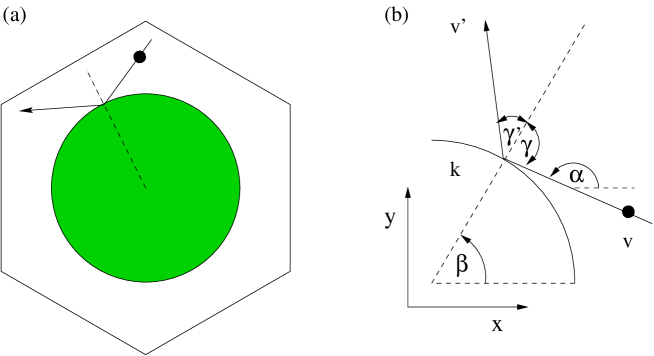
FIG. 1.: (a) Elementary cell of the periodic Lorentz gas on a triangular lattice. (b) Definition of the relevant variables to describe the collision process.

FIG. 2.: Probability densities for $d=3$ at $E=0.5$

FIG. 3.: Probability densities for $d=3$ (solid curve), $4$ (dashed curve) and $6$ (long dashed curve) at $E=0.5$

FIG. 4.: Probability densities for $d\to\infty$ at $T=0.5$

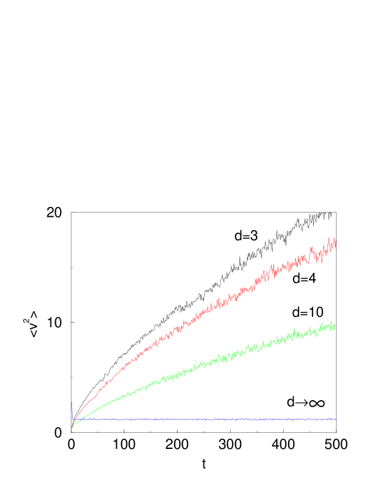
FIG. 5.: Time series of the ensemble average $<v^{2}>$ as a function of time $t$ for different d

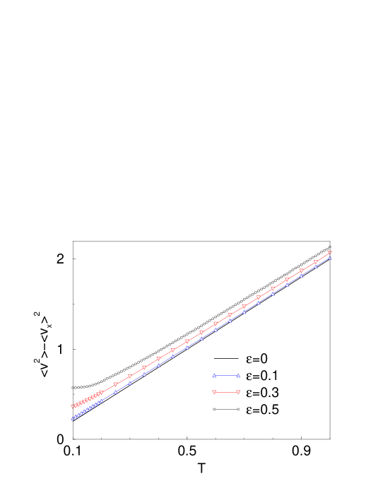
FIG. 6.: Relation between average velocity squared in the frame moving with the current, $<v^{2}>-<v_{x}>^{2}$, and parametric temperature $T$ for the infinite dimensional model. Equipartitioning of energy would imply $<v^{2}>-<v_{x}>^{2}=2T$. The numerical uncertainty of each point is less the size of the symbols

FIG. 7.: Probability densities for $d\to\infty$, $\varepsilon=0.5$ at $T=0.5$

FIG. 8.: Probability densities for $d\to\infty$ and $\varepsilon=0$ (solid curve), $0.5$ (dashed curve) and $1$ (long dashed curve) at $T=0.5$

FIG. 9.: Conductivity $\sigma(\varepsilon)$ as it varies with field strength $\varepsilon$ for $T=0.5$. The curve consists of 90 data points, the numerical uncertainty of each point is less the size of the symbols

FIG. 10.: (a),(b) Poincaré section of $(\beta,\sin\gamma)$ defined in Fig.1 at the moment of the collision for field strength $\varepsilon=1$. In (a) our model with the baker map has been used, in (b) the baker has been replaced by a random number generator. (c) Poincaré section of $\beta$ at the moment of the collision for varying field strength $\varepsilon$.(a).(b),(c) with $T=0.5$.

REFERENCES

- [1] W. G. Hoover and W. T. Ashurst, in Theoretical Chemistry, edited by H. Eyring and D. Henderson (Academic, New York, 1975), Vol. 1.
- [2] J. M. Haile and S. Gupta, J. Chem. Phys. 79, 3067 (1983).
- [3] M. D. Allen and D. J. Tildesley, Computer simulation of liquids (Clarendon Press, Oxford, 1987).
- [4] D. J. Evans and G. P. Morriss, Statistical Mechanics of Nonequilibrium Liquids (Academic Press, London, 1990).
- [5] W. G. Hoover, Computational statistical mechanics (Elsevier, Amsterdam, 1991).
- [6] S. Hess, in Computational physics, edited by K. Hoffmann and M. Schreiber (Springer, Berlin, 1996), pp. 268–293.
- [7] G. P. Morriss and C. P. Dettmann, Chaos 8, 321 (1998).
- [8] W. G. Hoover, A. J. C. Ladd, and B. Moran, Phys. Rev. Lett. 48, 1818 (1982).
- [9] D. J. Evans, J. Chem. Phys. 78, 3297 (1983).
- [10] D. J. Evans et al., Phys. Rev. A 28, 1016 (1983).
- [11] S. Nosé, Mol. Phys. 52, 255 (1984).
- [12] S. Nosé, J. Chem. Phys. 81, 511 (1984).
- [13] W. G. Hoover, Phys. Rev. A 31, 1695 (1985).
- [14] J. L. Lebowitz and H. Spohn, J. Stat. Phys. 19, 633 (1978).
- [15] A. Tenenbaum, G. Ciccotti, and R. Gallico, Phys. Rev. A 25, 2778 (1982).
- [16] S. Goldstein, C. Kipnis, and N. Ianiro, J. Stat. Phys. 41, 915 (1985).
- [17] R. Klages, K. Rateitschak, and G. Nicolis, preprint chao-dyn/9812021 (1998).
- [18] D. J. Evans and B. L. Holian, Phys. Rev. A 83, 4069 (1985).
- [19] B. Moran and W. G. Hoover, J. Stat. Phys. 48, 709 (1987).
- [20] B. L. Holian, W. G. Hoover, and H. A. Posch, Phys. Rev. Lett. 59, 10 (1987).
- [21] W. G. Hoover, Phys. Rev. A 37, 252 (1988).
- [22] G. P. Morriss, Phys. Lett. A 122, 236 (1987).
- [23] G. P. Morriss, Phys. Lett. A 134, 307 (1989).
- [24] W. G. Hoover and B. Moran, Phys. Rev. A 40, 5319 (1989).
- [25] G. P. Morriss, Phys. Rev. A 39, 4811 (1989).
- [26] W. G. Hoover and H. A. Posch, Chaos 8, 366 (1998).
- [27] W. G. Hoover and H. A. Posch, Phys. Lett. A 246, 247 (1998).
- [28] G. Eyink and J. Lebowitz, in Microscopic simulations of complex hydrodynamic phenomena, Vol. 292 of NATO ASI Series B: Physics, edited by M. Mareschal and B. L. Holian (Plenum Press, New York, 1992), pp. 323–326.
- [29] H. A. Posch and W. G. Hoover, Phys. Lett. A 123, 227 (1987).
- [30] H. A. Posch and W. G. Hoover, Phys. Rev. A 38, 473 (1988).
- [31] H. A. Posch and W. G. Hoover, Phys. Rev. A 39, 2175 (1989).
- [32] N. L. Chernov, C. L. Eyink, J. L. Lebowitz, and Y. G. Sinai, Phys. Rev. Lett. 70, 2209 (1993).
- [33] N. L. Chernov, C. L. Eyink, J. L. Lebowitz, and Y. G. Sinai, Comm. Math. Phys. 154, 569 (1993).
- [34] N. I. Chernov and J. L. Lebowitz, Phys. Rev. Lett. 75, 2831 (1995).
- [35] T. Tel, J. Vollmer, and W. Breymann, Europhys. Lett. 35, 659 (1996).
- [36] J. Vollmer, T. Tél, and W. Breymann, Phys. Rev. Lett. 79, 2759 (1997).
- [37] N. I. Chernov and J. L. Lebowitz, J. Stat. Phys. 86, 953 (1997).
- [38] G. Gallavotti and E. G. D. Cohen, Phys. Rev. Lett. 74, 2694 (1995).
- [39] D. Ruelle, J. Stat. Phys. 85, 1 (1996).
- [40] D. J. Evans, E. G. D. Cohen, and G. P. Morris, Phys. Rev. A 42, 5990 (1990).
- [41] W. N. Vance, Phys. Rev. Lett. 69, 1356 (1992).
- [42] A. Baranyai, D. J. Evans, and E. G. D. Cohen, J. Stat. Phys. 70, 1085 (1993).
- [43] C. Dellago, L. Glatz, and H. A. Posch, Phys. Rev. E 52, 4817 (1995).
- [44] J. R. Dorfman, An introduction to chaos in nonequilibrium statistical mechanics (Cambridge University Press, Cambrigde, 1999).
- [45] Chaos and Irreversibility, Vol. 8 of Chaos, edited by T. Tél, P. Gaspard, and G. Nicolis (American Institute of Physics, College Park, 1998).
- [46] Microscopic simulations of complex hydrodynamic phenomena, Vol. 292 of NATO ASI Series B: Physics, edited by M. Mareschal and B. L. Holian (Plenum Press, New York, 1992).
- [47] The microscopic approach to complexity in non-equilibrium molecular simulations, Vol. 240 of Physica A, edited by M. Mareschal (Elsevier, Amsterdam, 1997).
- [48] W. G. Hoover et al., Phys. Lett. A 133, 114 (1988).
- [49] C. P. Dettmann and G. P. Morriss, Phys. Rev. E 54, 2495 (1996).
- [50] C. P. Dettmann and G. P. Morriss, Phys. Rev. E 55, 3693 (1997).
- [51] P. Choquard, Chaos 8, 350 (1998).
- [52] C. Dellago and H. A. Posch, J. Stat. Phys. 88, 825 (1997).
- [53] P. Gaspard and G. Nicolis, Phys. Rev. Lett. 65, 1693 (1990).
- [54] P. Gaspard and J. R. Dorfman, Phys. Rev. E 52, 3525 (1995).
- [55] J. R. Dorfman and P. Gaspard, Phys. Rev. E 51, 28 (1995).
- [56] P. Gaspard, Chaos, Scattering, and Statistical Mechanics (Cambridge University Press, Cambridge, 1998).
- [57] H. A. Lorentz, Proc. Amst. Acad. 438 (1905).
- [58] L. A. Bunimovich and Y. G. Sinai, Commun. Math. Phys. 78, 479 (1981).
- [59] P. Cvitanovic, P. Gaspard, and T. Schreiber, Chaos 2, 85 (1992).
- [60] J. Machta and R. Zwanzig, Phys. Rev. Lett. 50, 1959 (1983).
- [61] P. Gaspard, Chaos 3, 427 (1993).
- [62] P. Gaspard and F. Baras, Phys. Rev. E 51, 5333 (1994).
- [63] G. P. Morriss and L. Rondoni, J. Stat. Phys. 75, 553 (1994).
- [64] P. Gaspard, Phys. Rev. E 53, 4379 (1996).
- [65] H. Matsuoka and R. Martin, J. Stat. Phys 88, 81 (1997).
- [66] J. Lloyd, L. Rondoni, and G. P. Morriss, Phys. Rev. E 50, 3416 (1994).
- [67] J. Lloyd, M. Niemeyer, L. Rondoni, and G. P. Morriss, Chaos 5, 536 (1995).
- [68] C. P. Dettmann and G. P. Morriss, Phys. Rev. E 54, 4782 (1996).
- [69] C. P. Dettmann and G. P. Morriss, Phys. Rev. Lett. 78, 4201 (1997).
- [70] K. Rateitschak and R. Klages (unpublished).
- [71] J. C. Maxwell, Cam. Phil. Trans. 12, 547 (1879).
- [72] L. Boltzmann, in Wissenschaftliche Abhandlungen von L. Boltzmann, edited by F. Hasenöhrl (J. A. Barth Verlag, Leipzig, 1909), Vol. 2, Chap. 63.
- [73] L. J. Milanović, H. A. Posch, and W. Thirring, Phys. Rev. E 57, 2763 (1998).
- [74] C. Wagner, R. Klages, and G. Nicolis, Phys. Rev. E 60, (in press) (1999).
- [75] N. van Kampen, Physica Norvegica 5, 279 (1971).
- [76] P. Gaspard and R. Klages, Chaos 8, 409 (1998).
- [77] W. Breymann, T. Tel, and J. Vollmer, Chaos 8, 396 (1998).
- [78] J. Groeneveld, priv. commun.
- [79] R. Klages and J. Groeneveld, Verhandl. DPG VI, 646 (1998).
- [80] R. Klages, Verhandl. DPG VI, 678 (1999).
- [81] R. Klages (unpublished).
- [82] H. A. Posch and W. G. Hoover, Phys. Rev. E 58, 4344 (1998).
- [83] K. Rateitschak, R. Klages, W. Hoover, and G. Nicolis (unpublished).
- [84] J. Lebowitz and H. Spohn, preprint cond-mat/9811220.
- [85] C. Dellago and H. A. Posch, Phys. Rev. E 52, 2401 (1995).
- [86] C. Dellago, H. A. Posch, and W. G. Hoover, Phys. Rev. E 53, 1485 (1996).
- [87] N. Brillantov, F. Spahn, J.-M. Hertzsch, and T. Pöschel, Phys. Rev. E 53, 5382 (1996).
- [88] T. Pöschel and T. Schwager, Phys. Rev. Lett. 80, 5708 (1997).
- [89] T. Schwager and T. Pöschel, Phys. Rev. E 57, 650 (1998).
- [90] G. Giese and A. Zippelius, Phys. Rev. E 54, 4828 (1996).
- [91] T. Aspelmeier, G. Giese, and A. Zippelius, Phys. Rev. E 57, 857 (1998).