Order and chaos in galactic maps

Abstract

We investigate the properties of motion in a map model derived from a galactic Hamiltonian made up of perturbed elliptic oscillators. The phase space portrait is obtained in all three different cases using the map and numerical integration of the equations of motion. Our numerical calculations suggest that the map describes very well the properties of regular motion in all three cases. There are cases where the map fails to describe chaotic motion and cases where the map describes satisfactorily the chaotic phase plane. We also compare the Lyapunov characteristic number and the spectra of orbits derived by the map and numerical integration in each case. The agreement of the outcomes is satisfactory.

1 Introduction

The application of modern methods in the domain of Galactic Dynamics has been proved very fruitful during the last decade. Among them is the use of maps to describe galactic motion (Caranicolas c1 (1990), c3 (1994)), and the invariant spectra in galactic Hamiltonian systems (see Contopoulos et al. cong (1995), Patsis et al. panos (1997)).

Maps, derived from galactic type Hamiltonians, are useful in the study of galactic orbits because they are faster, in general, than numerical integration and allow a quick visualisation of the corresponding phase plane. Maps also can give the stability conditions for the periodic orbits. On the other hand, our experience based on previous work shows that the results given by the maps are in good agreement with those given by numerical integration at least for small perturbations (see Caranicolas & Karanis ck (1999)). On this basis, it seems that one has some good reasons to use a map for the study of galactic motion.

In the present work we consider that the local (i.e. near an equilibrium point ) galactic motion is described by the potential

$$V=\frac{1}{2}\left(\omega_{1}^{2}x^{2}+\omega_{2}^{2}y^{2}\right)-\epsilon\left[\beta\left(x^{4}+y^{4}\right)+2\alpha x^{2}y^{2}\right]\leavevmode\nobreak\ \leavevmode\nobreak\ ,$$ (1)

where $\omega_{1},\omega_{2}$ are the unperturbed frequencies of oscillation along the x and y axis respectively, $\epsilon>0$ is the perturbation strength while $\alpha,\beta$ are parameters.We shall study the case where $\omega_{1}=\omega_{2}=\omega$. Without the loss of generality we can take $\omega=1$, that is the 1:1 resonance case. Then the Hamiltonian to the potential (1) is

$$H = \frac{1}{2}\left(p_{x}^{2}+p_{y}^{2}+x^{2}+y^{2}\right)$$ (2)

$$-\epsilon\left[\beta\left(x^{4}+y^{4}\right)+2\alpha x^{2}y^{2}\right]=h\leavevmode\nobreak\ \leavevmode\nobreak\ ,$$

where $p_{x},p_{y}$ are the momenta per unit mass conjugate to x, y and h is the numerical value of H.

Our aim is to study the various types of periodic orbits, their stability and the kind of non periodic motion (regular or chaotic) in the Hamiltonian (2) for various values of parameters $\alpha$ and $\beta$ using the map corresponding to the Hamiltonian (2), as well as numerical integration. This resonance case is also known as the perturbed elliptic oscillators (Deprit d1 (1991), Deprit & Elipe d2 (1991), Caranicolas & Innanen ci (1992), Caranicolas c2 (1993)). The $x-p_{x}$ Poincare phase plane derived by the map and the numerical integration will be compared in each case. Of a special interest is the study of the chaotic motion. We shall try to find an answer to questions such as:

1. Does the map describe in a satisfactory way the chaotic layers in the $x-p_{x}$ plane and, if so, how this behavior evolves by increasing $\epsilon$ ?

2. What are the differences, if any, in the Lyapunov Characteristic Number (LCN) found by the map and the numerical integration in the regular and the chaotic area?

3. Are there any similarities in the invariant spectra derived by the map and the numerical integration?

The map and the stability conditions of the periodic orbits are given in Section 2. In the same Section we compare the $x-p_{x}$ phase plane found by the map and numerical integration for some of the main different cases. In Section 3 we compare the LCNs and the spectra of orbits, derived using the map and numerical integration. Section 4 is devoted to a discussion and the conclusions of this work.

2 Map and stability conditions

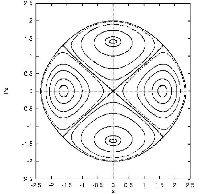
Figure 1: The $x-p_{x}$ (type A) phase plane derived by numerical integration. The values of the parameters are $\alpha=1.2$, $\beta=0.8$, $\epsilon=\epsilon_{esc}=0.03125$, $h=2$.

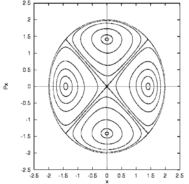
Figure 2: Same as Fig. 1 derived by the map.

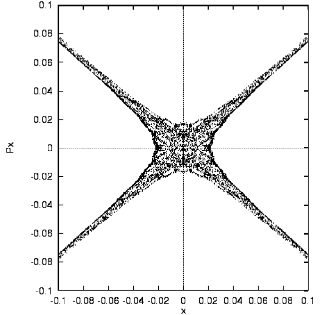
Figure 3: The area near the center of Fig. 1

The averaged Hamiltonian corresponding to the Hamiltonian (2) reads

$$<H> = \epsilon\alpha J\left(\Lambda-J\right)\left[2-\cos 2\phi\right]$$ (3)

$$+\frac{3}{2}\epsilon\beta\left[J^{2}+\left(\Lambda-J\right)^{2}\right]$$

Following the steps described in Caranicolas (c1 (1990)) we find the map

$$J_{n+1} = J_{n}-2\epsilon\alpha J_{n+1}(\Lambda-J_{n+1})\sin 2\phi_{n}$$

$$\phi_{n+1} = \phi_{n}+\epsilon(2\alpha-3\beta)(\Lambda-2J_{n+1})$$

$$-\epsilon\alpha(\Lambda-2J_{n+1})\cos 2\phi_{n}$$

where $\Lambda=h$. The map describes the motion in the $J-\phi$ plane and we return to $x,p_{x}$ variables through $x=(2J)^{1/2}\cos\phi,p_{x}=-(2J)^{1/2}\sin\phi$. The fixed points of (4) are at

$$(i)\ \ \ J = 0,\ \ \ \ \ \ \ \ for\ \ \ any\ \ \ \phi$$

$$(ii)\ \ \ J = \Lambda/2,\ \ \ \ \phi=0,\pi$$ (5)

$$(iii)\ \ \ J = \Lambda/2,\ \ \ \ \phi=\pm\pi/2\leavevmode\nobreak\ \leavevmode\nobreak\ .$$

There are three distinguished case of the $x-p_{x}$ phase plane portrait in the Hamiltonian (2). Type A, when both fixed points (i) and (ii) are stable. Type B when points (i) are stable while fixed points (ii) are unstable. In type C phase plane, fixed points (i) and (ii) are unstable and stable respectively. Applying the stability conditions (see Lichtenberg & Lieberman ll (1983)) we find after some straightforward calculations: Type A phase plane appears when $\alpha>\beta>\alpha/3$ $(\alpha>0,\beta>0)$. Type B appears when $\beta>\alpha$ $(\alpha>0,\beta>0)$. We observe the phase plane of type C when $\alpha>3\beta$ $(\alpha>0,\beta>0)$ or if $\alpha<0,\beta>0$.

In all three cases there is, for a fixed value of the energy h, a value of the perturbation strenght $\epsilon_{\mathrm{esc}}$, such as for $\epsilon>\epsilon_{\mathrm{esc}}$ curves of zero velocity $h-V=0$ open and the test particle is free to escape. We do not consider cases where the curves of zero velocity are always closed that is cases where the Hamiltonian (1) has no $\epsilon_{\mathrm{esc}}$. The value of $\epsilon_{\mathrm{esc}}$ can be found using the method described in Caranicolas & Varvoglis (cvar (1984)). For the type A phase plane we find

$$\epsilon_{\mathrm{esc}}=1/[8h(\alpha+\beta)]\leavevmode\nobreak\ \leavevmode\nobreak\ ,$$ (6)

while in the cases B and C $\epsilon_{\mathrm{esc}}$ is given by the formula

$$\epsilon_{\mathrm{esc}}=1/[16h\beta]\leavevmode\nobreak\ \leavevmode\nobreak\ .$$ (7)

Let us now go to see the three different types of the phase plane produced by the Hamiltonian system (2). In all numerical calculation we use the value $h=2$. Fig. 1 shows the type A $x-p_{x}$ phase plane derived by numerical integration. The values of $\alpha,\beta$ are 1.2, 0.8 respectively while $\epsilon=\epsilon_{\mathrm{esc}}=0.03125$. The motion is everywhere regular except near the hyperbolic point in the center and in a thin strip along the separatrix.(see Fig. 3). Fig. 2 is the corresponding figure produced by the map. As one can see the agreement is good. One significant difference is that the map is inadequate to produce the chaotic layer seen in Fig. 3. Also note that $x_{max}$ in Fig. 1 is greater than 2 while in Fig. 2 is smaller.

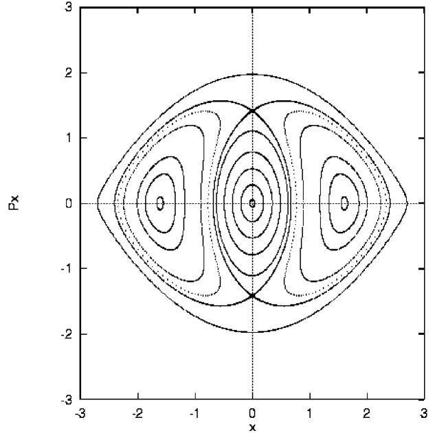
Figure 4: The $x-p_{x}$ (type B) phase plane derived by numerical integration. The values of the parameters are $\alpha=0.2$, $\beta=0.25$, $\epsilon=\epsilon_{esc}=0.125$, $h=2$.

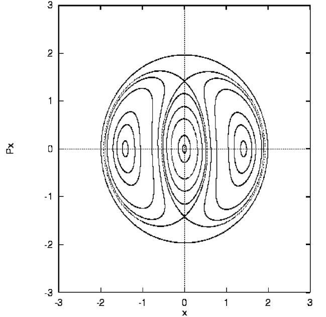
Figure 5: Same as Fig.4 derived by the map.

Fig. 4 and Fig. 5 show the type B phase plane derived using numerical integration and the map respectively. The values of the parameters are $\alpha=0.20$, $\beta=0.25$, while $\epsilon=\epsilon_{\mathrm{esc}}=0.125$. The results are similar to those observed in Figs. 1 and 2. Again the map describes well the real phase plane except in a small chaotic region near the two hyperbolic fixed points. Thus, our numerical calculations suggest that, the map (4) describes well the properties of motion in the Hamiltonian (2) up to the largest perturbation, that is $\epsilon=\epsilon_{\mathrm{esc}}$ but it is insufficient to described the small chaotic region observed when using numerical integration.

Type C phase plane is shown in Figs. 6 and 7. Fig. 6 comes from numerical integration while Fig. 7 was derived using the map. The values of the parameters are $\alpha=-1.20,\beta=0.20$, while $\epsilon=\epsilon_{\mathrm{esc}}=0.15625$. This value of $\epsilon$ was chosen to maximize the chaotic effects. The most important characteristic, observed in both Figs. 6 and 7 is the large unified chaotic region. In contrast with the two previous cases A and B, here the map reproduces satisfactorily the chaotic sea found by numerical integration. On the other hand, it is evident that the map describes qualitatively in a satisfactory way the areas of regular motion around the elliptic points in the $p_{x}$ axis. Some differences are observed in the area near the center between the two patterns. Another important characteristic, observed in case C, is that the chaotic areas are large even when $\epsilon<\epsilon_{\mathrm{esc}}$. Results, not shown here, suggest that considerable chaotic areas are observed in the phase plane derived using the map, when $\epsilon\geq 0.08$. Therefore we must admit that our numerical experiments show that, in the case when the Hamiltonian system (2) has small chaotic regions, the map is inadequate to produce them but it describes them satisfactorily when they are large.

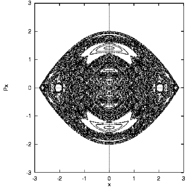
Figure 6: The $x-p_{x}$ (type C) phase plane derived by numerical integration. The values of the parameters are $\alpha=-1.2$, $\beta=0.2$, $\epsilon=\epsilon_{esc}=0.15625$, $h=2$.

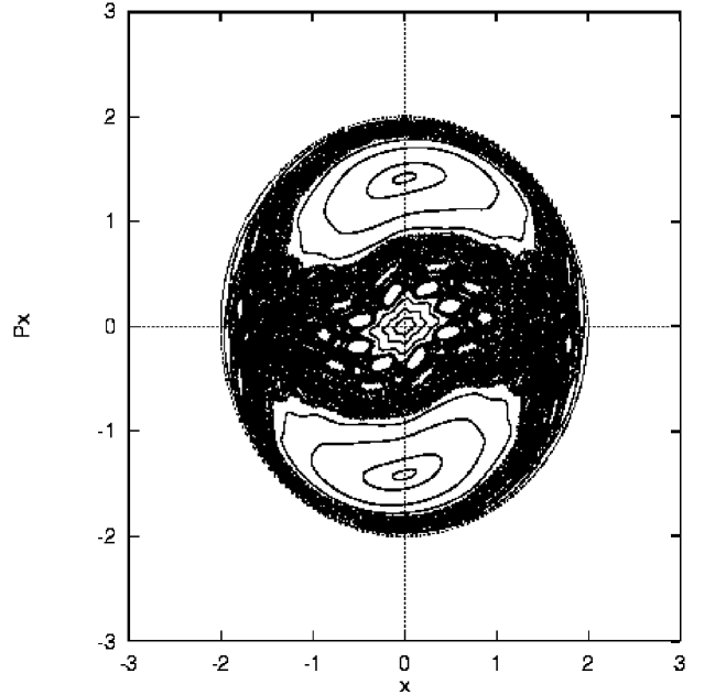
Figure 7: Same as Fig.6 derived by the map.

3 Dynamical spectra

In this Section we shall study the spectra of the Hamiltonian system (2) using numerical integration and the map (4).Before doing this, it is necessary to remember some useful notions and definitions. The “stretching number” $\alpha_{i}$ (see Voglis & Contopoulos vogcon (1994), Contopoulos at al. cong (1995), Contopoulos & Voglis conv (1997)) is defined as

$$\alpha_{i}=\ln\left|\frac{\xi_{i+1}}{\xi_{i}}\right|\leavevmode\nobreak\ \leavevmode\nobreak\ ,$$ (8)

where $\xi_{i+1}$ is the next image on the Poincare phase plane of an infinitesimal deviation $\xi_{i}$ between two nearby orbits. The spectrum of the stretching numbers is their distribution function

$$S(\alpha_{i})=\frac{\Delta N(\alpha)}{Nd\alpha}\leavevmode\nobreak\ \leavevmode\nobreak\ ,$$ (9)

where $\Delta(\alpha)$ is the number of stretching numbers in the interval $(\alpha,\alpha+d\alpha)$ after N iterations.The maximal Lyapunov characteristic number can be written as

$$LCN=\int\limits_{-\infty}^{\infty}\alpha S(\alpha)d\alpha\leavevmode\nobreak\ \leavevmode\nobreak\ ,$$ (10)

in other words, the LCN is the average value of the stretching number $\alpha$.

Today we know that the distribution of the successive stretching numbers forms a spectrum which is invariant with respect to (i) the initial conditions along an orbit and the direction of the deviation from this orbit and (ii) the initial conditions of the orbits belonging to the same chaotic region.

In what follows we shall give the spectra $S(\alpha)$ of orbits of the Hamiltonian system (2) derived using the map (4) as well as numerical integration. In the case of the Hamiltonian where t is a continuous quantity ( that is in the numerical integration of the equations of motion) we use for the derivation of the stretching numbers and spectra the method used by Contopoulos et al. (1995). All calculations correspond to the case C because the results are much more interesting.

Figure 8: The spectrum $S(\alpha)$ of two chaotic orbits derived using numerical integration. The values of the parameters are as in Fig. 6. Initial conditions $x=1.3$, $y=p_{x}=0$ and $x=1.1$, $y=0$, $p_{x}=0.2$. The value of $p_{y}>0$ is found from the energy integral.

Figure 9: Same as Fig. 8 derived using the map.

Figure 10: LCNs for the same chaotic orbit given by the map 1 and numerical integration 2. Initial conditions $x=1.3$, $y=p_{x}=0$.

Fig. 8 shows the spectra of two orbits (the first with solid line the other with dots) derived using numerical integration. The orbits were started in the chaotic region with different initial conditions. It is evident that the two spectra are close to each other. Fig. 9 shows the spectra of the same two orbits found using the map. Again the two spectra are close to each other. The spectra in both cases were calculated for $N=10^{6}$ periods. As one observes the pattern shown in both Figs. 8 and 9 have the characteristics of the spectrum of orbits belonging to a chaotic region. Fig. 10 shows the LCNs for two chaotic orbits. Number 1 was derived using the map, while number 2 was found using numerical integration. As one can see the mean exponential divergence of the two nearby chaotic trajectories, described by the map, is larger than that given by numerical integration. Nevertheless the two curves are qualitatively similar.

In Figs. 11 and 12 we give the spectra of the same regular orbit derived by numerical integration and the map respectively. This is an orbit with initial conditions near the periodic orbit $x=y=0,p_{x}=\Lambda^{1/2}$. The spectra were calculated for $N=10^{6}$ periods. As one can see the agreement between the two spectra is good. From other cases we know that the agreement is much better if we calculate an orbit for $N=10^{7}$, or $N=10^{8}$ periods. Both are “U-shaped”, with two large and two small peaks. Such spectra are characteristic of quasi-periodic orbits, starting close to a stable periodic orbit (see Patsis et al. panos (1997)). Fig. 13 shows the LCNs for the orbit of Fig. 11 derived using a map (dots) and numerical integration (solid line). Again one can see that the map describes well the qualitative properties of regular orbits.

Let us now come to the symmetry of the spectra. It was observed that the spectra of ordered orbits, starting close to a stable periodic orbit, are almost symmetric with respect to the $\alpha=0$ axis, while, when we go far from the stable periodic orbit they become asymmetric. In order to give an estimate between closeness and symmetry we have made extensive numerical experiments near the exact periodic orbit $x=0$, $p_{x}=h^{1/2}=\sqrt{2}$.

Figure 11: The spectrum $S(\alpha)$ of a regular orbit derived using numerical integration. The values of the parameters are as in Fig. 6. Initial conditions $x=y=0$, $p_{x}=1.55$. The value of $p_{y}>0$ is found from the energy integral.

Figure 12: Same as Fig. 11 derived using the map.

Figure 13: LCNs for the same regular orbit given by the map (dots) and numerical integration (solid line). Initial conditions as in Fig 11.

We define as “symmetry factor” the quantity

$$Q=\frac{1}{N}\sum_{i=1}^{N}|S(\alpha_{i})-S(-\alpha_{i})|$$ (11)

As one can see, $Q=0$ corresponds to a perfectly symmetric spectrum, while $Q=1$ to a totally asymmetric with all non zero values of $S(\alpha)$ to belong to either positive or negative $\alpha$. The results $Q$ vs $p_{x}$ for the map, in the case C, when $\epsilon=0.02$, are shown in Fig. 14. Dots correspond to values given by the numerical experiments, while the solid line corresponds to the best fit

$$Q\leavevmode\nobreak\ =\leavevmode\nobreak\ \mathrm{a}p_{x}^{2}+bp_{x}+c\leavevmode\nobreak\ \leavevmode\nobreak\ \leavevmode\nobreak\ ,$$ (12)

where $\mathrm{a}=0.2704$, $b=-0.7960$ and $c=0.5986$. Fig. 15 is the same as Fig. 14, for the Hamiltonian in the case C when $\epsilon=0.1$. The best fit is now with $\mathrm{a}=0.9100$, $b=-2.659$ and $c=1.983$. As we can see we have a second order polynomial growth of the asymmetry of the spectrum as we move far from the stable periodic orbit. The value of N in all cases was $10^{6}$ iterations.

4 Discussion

In this paper we have studied the regular and chaotic motion in the Hamiltonian system (2) using a map, derived from the averaged Hamiltonian and numerical integration. Note that Hamiltonian (2) is integrable when $\alpha=\beta$ and when $\alpha=3\beta$. Depending on the choice of the parameters $\alpha,\beta$ this Hamiltonian displays three different types of $x-p_{x}$ phase plane named as types A,B,C. In the case of the two first types of phase plane, the map describes in a very satisfactory way the real properties of orbits up to $\epsilon=\epsilon_{\mathrm{esc}}$. Extensive numerical calculations have shown that the map does not produce any chaotic regions in the cases A and B. Therefore, one concludes that the map fails to describe the small chaotic regions near the separatrix found by numerical integration. Here we must note that at the beginning we had started with smaller values of $\epsilon$, but we observed that the map persisted not to produce chaos up to $\epsilon=\epsilon_{\mathrm{esc}}$. This explains why $\epsilon=\epsilon_{\mathrm{esc}}$ was chosen.

Figure 14: $Q$ vs $p_{x}$ for the map in case C, when $\epsilon=0.02$

Figure 15: Same as Fig. 14 for the Hamiltonian in case C when $\epsilon=0.1$.

The situation is quite different in the case of the phase plane of type C. Here the system has large chaotic regions, increasing when $\epsilon$ approaches $\epsilon_{\mathrm{esc}}$ and the map describes them satisfactorily. Moreover, the comparison of the spectra and LCNs of orbits found using the map and numerical integration shows that one can trust the map. This is very important because the map is at least 10-20 times faster than numerical integration and one can make faster all the time consuming calculations. Note that in all cases the number of periods in the calculation of the spectra using the map or numerical integration was the same in order to be able to compare the corresponding results.

We have also investigated the symmetry of the spectra of ordered orbits. It was found that the quantity $Q$ increases, with a second order polynomial dependence, as we are moving far from the stable periodic orbit.

Finally the authors would like to make clear that (i) the proposed map has some qualitative similarities with the Poincaré map of the original Hamiltonian system (2), although the numerical differences may be important and (ii) the results of this work correspond to the particular Hamiltonian system (2) and for the resonance case 1:1. Interesting results, on the spectra of orbits, in galactic Hamiltonians made up of harmonic oscillators in the 4:3 resonance, have been given by Contopoulos et al. (cong (1995)). Also spectra of orbits have been studied, in the standard map, by Voglis & Contopoulos (vogcon (1994)), Contopoulos et al. (conve (1997)). This paper was focused on the comparison of the results (structure of the phase plane and spectra of orbits) given by numerical integration and the map.

- (1) Caranicolas, N.D., 1990, Cel. Mech. 47, 87
- (2) Caranicolas, N.D., 1993, A&A 267, 368
- (3) Caranicolas, N.D., 1994, A&A 291, 754
- (4) Caranicolas, N., Varvoglis, Ch., 1984, A&A 141, 383
- (5) Caranicolas, N.D, Innanen, K.A., 1992, AJ 103, 1308
- (6) Caranicolas, N.D. ,Karanis, G.I., 1999, A&A 342, 389 304, 374
- (7) Contopoulos, G., Voglis, N., 1997,A&A 317, 73
- (8) Contopoulos, G., Grousousakou, E., Voglis, N. 1995 A&A
- (9) Contopoulos, G., Voglis, N., Efthymiopoulos, C., Froeschle, C., Gonczi, R., Lega, E., Dvorak, R., Lohinger, E., 1997, Cel. Mech. 67, 293
- (10) Deprit, A., 1991, Cel. Mech. 51, 203
- (11) Deprit, A., Elipe, A., 1991, Cel. Mech. 51, 227
- (12) Lichtenberg, A. J., Lieberman, M. A., 1983, Regular and stochastic motion, Springer, Berlin Heidelberg, New York
- (13) Patsis, P. A., Efthymiopoulos, C., Contopoulos, G., Voglis, N., 1997, A&A 326, 493
- (14) Voglis, N., Contopoulos, G., 1994, J.Phys. A 27, 4899