Imperfect fractal repellers and irregular families of periodic orbits in a 3-D model potential

Abstract

A model, plane symmetric, 3-D potential, which preserves some features of galactic problems, is used in order to examine the phase space structure through the study of the properties of orbits crossing perpendicularly the plane of symmetry. It is found that the lines formed by periodic orbits, belonging to Farey sequences, are not smooth neither continuous. Instead they are deformed and broken in regions characterised by high Lyapunov Characteristic Numbers (LCN’s). It is suggested that these lines are an incomplete form of a fractal repeller, as discussed by Gaspard and Baras (1995), and are thus closely associated to the “quasi-barriers” discussed by Varvoglis et al. (1997). There are numerical indications that the contour lines of constant LCN’s possess fractal properties. Finally it is shown numerically that some of the periodic orbits -members of the lines- belong to true irregular families. It is argued that the fractal properties of the phase space should affect the transport of trajectories in phase or action space and, therefore, play a certain role in the chaotic motion of stars in more realistic galactic potentials.

1 Introduction - Motivation

One of the most interesting open questions in non-linear dynamics is the nature and evolution of transport in the chaotic phase space regions of perturbed integrable Hamiltonian systems. Most of the work in this field has been done for 2-D systems or for the standard map, following two different approaches. In the first approach, which may be designated as microscopic, one studies the homoclinic and heteroclinic tangle of stable and unstable manifolds inside the chaotic region. This gives a “complete” qualitative picture of transport in phase space, since a chaotic trajectory follows the unstable manifolds of the unstable periodic orbits, jumping from one to another near the heteroclinic points. On the other hand, invariant tori surrounding stable periodic orbits act as “barriers” in the transport process, modifying at the same time the topological structure of phase space. However, it is not presently well understood how the results from this kind of study can be used in a quantitative description of the evolution of an ensemble of trajectories.

In the second approach, which may be designated as macroscopic, one assumes a priori that transport is a pure random phenomenon (a Markovian process). Then the transport of an ensemble of trajectories may be considered as “classical diffusion” in action space. Unfortunately, it is well known that transport in Hamiltonian systems cannot be considered as a pure Markovian process, due to the problem of stickiness. Moreover the process may follow Lévy rather than classical statistics (Shlesinger et al., 1993). In this case the macroscopic approach still works, provided that the process is considered as fractal diffusion in normal space (Zaslavsky, 1994). In this way it becomes evident that Lévy-like statistics are closely related to the self-similarity of the phase space. This formalism results in a differential equation with fractional partial derivatives, whose solution is formidably difficult, even in the simple case of 2-D systems.

There are rather few attempts to study transport in Hamiltonian systems with more than two degrees of freedom, mainly because the above mentioned approaches for 2-D systems cannot be directly generalized. It is therefore important to note that there exists yet a third approach for the description of transport, which may be implemented in a straightforward way in systems with more than two degrees of freedom, and this is normal diffusion in fractal space (e.g. see West and Deering, 1994, and references therein). The fractality of phase space has been already demonstrated for 2-D systems and has been associated with the self similarity of the hierarchical structure of island families on a surface of section (e.g. see Zaslavsky, 1994, BenKadda et al., 1997).

In the case of more than two degrees of freedom the situation is more complicated, since the topological structure of phase space in any region depends on the number of local integrals of motion. Recently Varvoglis et al. (1997) have found indications of phase space fractality in the same model 3-D Hamiltonian system studied in the present work, but they were unable, due to the particular method of study they had selected, to identify actual fractal or multifractal sets in phase space. They have conjectured that the fractality is due to the presence of quasi-barriers (Varvoglis and Anastasiadis, 1996), i.e. geometrical objects of lower than full dimensionality (depending on the number of local integrals of motion), such as periodic orbits, invariant tori around them and cantori (Aubry, 1978; Percival, 1979).

From the above discussion it is obvious that the importance of the fractality of phase space in the diffusion process lies in the nature and in the rate of the diffusion: In a simply connected space, the diffusion is classical and follows Fick’s law (transport proportional to $\sqrt{(}t)$). In a fractal space the diffusion is non-classical (presumably a Lévy process) and, in the case of a Hamiltonian system, usually it has a lower than the Fickian rate.

On the other hand, the distribution of periodic orbits perpendicular to the $x-y$ plane in the present 3-D model potential has been studied by Barbanis and Contopoulos (1995) (henceforth referred to as BC) and Barbanis (1996). It was found that it is not random: the perpendicular crossings (p.c.’s) of orbits with multiplicities forming Farey sequences with the $x-y$ plane are arranged along lines, named in the present paper basic-lines (BL) and Farey tree lines (FTL). These lines are not continuous but they possess gaps; two of them have already been mentioned in BC. Since the presence of Farey sequences implies a form of self-similarity, it is possible that the BL’s and FTL’s may be related to the above-mentioned quasi-barriers and that the gaps may be related to any fractal properties of phase space.

In the present paper we use the model potential studied by BC in order to test the conjecture put forward by Varvoglis et al. (1997) about the origin of the fractality of phase space. Furthermore, through this, we attempt to assess the relation between the topological structure of the phase space and transport, on the one hand, and the system of BL’s and FTL’s, on the other. Although this potential can model a true galaxy only locally, its study is expected, nevertheless, to contribute to the understanding of galactic evolution problems, based on the fact that evolution is intimately connected to transport in phase and configuration space. Transport in a chaotic region of a perturbed integrable dynamical system, in turn, may be viewed as (stochastic) diffusion, which depends on the value of the Lyapunov Characteristic Number as well as on the topological structure of the phase space. We believe that similar behaviour would characterise any 3-D perturbed integrable dynamical system, as are most of the realistic model galactic potentials.

The purpose of this paper is threefold:

(a) to study in finer detail the distribution of the periodic orbits along the BL’s and FTL’s.

(b) to examine whether these lines are connected, in any way, to transport in phase space and are, thus, related to the “quasi-barriers” and

to confirm the existence of true irregular families of periodic orbits in a 3-D Hamiltonian system.

This paper is organized as follows. In the next section we present, for reasons of completeness, some remarks on previous results. In Section 3 we show that the LCN’s may “map” the fractality of phase space. In Section 4 we present our results on the interconnection and discontinuities of BL’s and FTL’s. In Section 5 we show numerically the existence of irregular families of periodic orbits. Finally in Section 6 we summarise and discuss our results.

2 Remarks on previous results

2.1 Basic lines

The systematic exploration of the phase space structure of 3-D Hamiltonian systems was initiated by Magnenat (1982) and later by Contopoulos & Barbanis (1989), BC and Barbanis (1996), through the study of periodic orbits of unit mass test particles in a 3-D model potential, corresponding to the Hamiltonian

$$H= {1\over 2}\left(p_{x}^{2}+p_{y}^{2}+p_{z}^{2}\right)+{1\over 2}\left(Ax^{2}+By^{2}+Cz^{2}\right)$$

$${-\epsilon xz^{2}-\eta yz^{2}=h}$$

with a particular set of parameters (A = 0.9, B = 0.4, C = 0.225, $\epsilon=0.560$, $\eta=0.20$ and $h=0.00765$). The specific values for the parameters A, B, C were selected by Magnenat (1982) because the 2-D system $x-z$ for $\sqrt{A/C}$ = 2 is topologically equivalent to the Inner Lindblad Resonance and the 2-D system $y-z$ for $\sqrt{B/C}$ = 4/3 is a well studied 2-D dynamical system with extended chaotic regions. For this set of parameters it was found in BC that the distribution of the p.c.’s of the periodic orbits is not accidental: the crossings are arranged along particular lines on the $\overline{x}-\overline{y}$ plane (where $\overline{x}=A^{1/2}x$, $\overline{y}=B^{1/2}y$), as it is evident in Fig. 1 (taken from Fig. 5 of BC). Each orbit has either one p.c., marked by a (x), or two p.c.’s, marked by (+). In this paper, for clarity reasons, we use a point ($\cdot$) instead of (x). Each p.c. is designated by a number (or a number and a letter), representing the multiplicity of the orbit; different orbits with the same multiplicity are differentiated by a prime. The lines are formed by the p.c.’s of the orbits, whose multiplicities form arithmetic progressions with increment the multiplicity of the limit orbit. They are termed in this paper basic if they connect orbits of the unperturbed system (e.g. 1a, 1b in Fig. 1) or orbits with low multiplicity, $m$ (e.g. $m\leq 5$). For example the basic sequences

• 3(+), 5($\cdot$), 7(+), 9($\cdot$), …2c(+)

• and 3(+), 5^′($\cdot$), 7(+), 9^′($\cdot$), …2c(+),

which form the lines C and C^′, start with an orbit of multiplicity 3 and increment 2, which is the multiplicity of the limit orbit 2c.

2.2 Farey tree lines

In BC it was recognized that the distribution of p.c.’s on the $\overline{x}-\overline{y}$ plane presents some self-similar features. To begin with, to each basic sequence of orbits corresponds a number of new sequences of higher order. Each member of a new sequence is a periodic orbit having as multiplicity the sum of the multiplicities of two consecutive orbits of the generating sequence. For example between the first two orbits of the basic sequence C, i.e. 3(+) and 5($\cdot$), there is the orbit 8(+). Two second order sequences are formed between 3 and 8 as well as between 8 and 5, i.e.

$$8(+),11(\cdot),14(+),17(\cdot),20(+),23(\cdot),...3(\cdot)$$

$$\mathrm{and}$$

$$8(+),13(+),18(+),23(+),28(+),...5(\cdot)$$

Both new sequences have as first member the orbit 8, but they have different limit orbits and increments (i.e. 3 for the first and 5 for the second, respectively). In the same way we can form sequences of even higher order. We call the orbits of these higher order sequences Farey tree orbits and the lines on which they lie Farey tree lines, because such sequences are similar to the Farey sequences discussed by Niven and Zuckerman (1960). For a good review on Farey trees see Efthymiopoulos et al. (1997).

The periodic orbits are used, in the present paper, as an additional tool for probing the topological structure of the phase space. In particular, periodic orbits of high multiplicities are needed in order to search for self-similar structures in the BL’s and FTL’s for a wide interval of multiplicities (see Avnir et al., 1998). The importance of the non-basic (Farey) lines lies exactly on the above line of reasoning, as well as in the fact that they might be necessary in order to calculate correctly an appropriate diffusion coefficient. It should be noted that we have restricted our study to the periodic orbits crossing perpendicular the x-y plane for simplicity reasons.

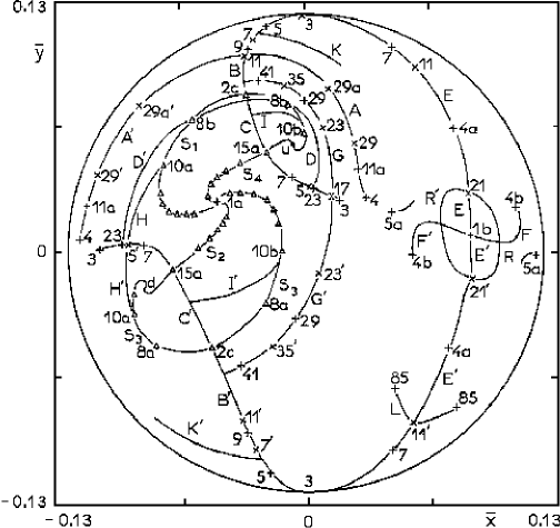
Figure 1: The majority of the perpendicular crossings of the periodic orbits of the Hamiltonian (1) lie on particular lines on the $\overline{x}-\overline{y}$ plane inside the boundary circle $\overline{x}^{2}+\overline{y}^{2}=2h$. Most of the lines are concentrated around the basic orbits 1a and 1b. There is also a noticeable spiral structure with focal point the orbit 1a. Four spirals illustrate the area of this structure. Note that in this figure (reproduced from BC, Fig. 5) a different notation is used than in the rest of the present paper. Each symbol, $(\times)$ or $(+)$, shows a periodic orbit with one or two crossing points, respectively.

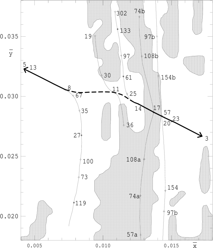
Figure 2: A segment of the BL between the p.c.’s of the periodic orbits 3 and 5 (indicated by a bold line) and the network of various FTL’s (corresponding to the upper central part of Fig. 1, line C). The nonexistent part of C between 8 and 14 is indicated by a dashed line. The contour lines of constant LCN’s $\lambda=10^{-4}$ are superimposed and the regions of $\lambda>10^{-4}$ are gray shaded

2.3 Irregular orbits

All periodic orbits of the same multiplicity that can be found through the continuous variation of a parameter in the equations of motion belong to the same family. The graph giving one of the initial conditions of the periodic orbits as a function of the parameter is the characteristic of this family. Families, which do not exist for values of the perturbing parameter below a critical value, appear only as pairs, are well known in 2-D dynamical systems and are called irregular families (Contopoulos 1970; Barbanis 1986). However, their existence has not been proven for 3-D systems. Pairs of families that have been found in such systems without a direct connection to a basic orbit, they were all of small multiplicities and it turns out that they have an indirect connection to a basic orbit through other families bifurcating from it (Barbanis, 1996). It is desirable to know whether families of periodic orbits in 3-D systems (presumably of high multiplicities) do exist without any connection to a basic orbit. Their presence might play a certain role in the fractality of phase space and, therefore, in trajectory transport.

2.4 Lyapunov Numbers

Varvoglis et al. (1997), while studying numerically transport phenomena in the trajectories of the Hamiltonian (1), have found, in an indirect way, that the phase space shows a fractal structure. In particular they presented numerical evidence that the function $dV/dt$ has multifractal properties, where $V(t)$ denotes essentially the coarse-grained volume of phase space visited by a trajectory up to time $t$. They found, also, that the evolution of the function $dV/dt$ is closely related to the evolution of the function

$$\chi(t)={1\over t}\ln{d(t)\over d(0)}$$ (3)

whose limit, as $t\rightarrow\infty$, is defined as the LCN. The function $\chi(t)$ shows plateaus in the time intervals where $dV/dt$ is close to zero and steeply increasing transient segments in the time intervals where $dV/dt$ takes large positive values. This fact shows that a trajectory is confined successively in regions of phase space where the LCN converges to a limit and, therefore, the fractal properties of $dV/dt$ should arise from the (apparently) self-similar distribution of periodic orbits and other quasi-barriers in phase space (Zaslavsky, 1994).

It should be emphasised that, in the present paper, LCN’s are not calculated in order to estimate “rates of diffusion”, since LCN’s alone cannot describe completely this phenomenon in the case where there exist invariant tori of considerable measure. We do, however, calculate LCN’s in order to “probe” the phase space structure, i.e. to delineate, in an independent from other methods way, the “topology” of the phase space. This new method is based on the property that trajectories starting in a certain region, bounded by “quasi-barriers”, are characterised by a certain “Local Lyapunov Number”. By drawing the contour lines of LCN’s, one draws, essentially, the geometric boundary of the region bounded by the “quasi-barriers”.

3 LCN’s and fractal properties

The “classical” calculation of LCN’s requires a continuous integration of the corresponding trajectories, until the function $\chi(t)$ has reached a plateau. It is, therefore, obvious that this method cannot be used in a “mass production” procedure. For this reason we decided to use a different approach, by calculating the value of the function $\chi(t)$ at various integration time intervals, $\Delta t$, up to $\Delta t=3\,10^{5}$. Comparing the results for different $\Delta t^{\prime}s$ we have found that they are qualitatively the same (i.e. they form level lines with increasing complexity as one goes to finer details), provided that $\Delta t>10^{5}$. So, even if $\chi(t)$ does not reach a plateau, its value at the end of the corresponding time interval $\Delta t>10^{5}$ gives a correct estimate, at least to order of magnitude, of the “degree of stochasticity” of the trajectory in the phase space region restricted by the quasi-barriers. We designate this value as the Fixed Time LCN. In what follows we use, for convenience, the notation LCN. Through this kind of LCN’s we attempt to probe the topological structure on the $\overline{x}-\overline{y}$ plane as follows:

We draw a dense mesh on the $\overline{x}-\overline{y}$ plane (for $0<\overline{x}<0.020$ and $0.010<\overline{y}<0.045$ at intervals $\Delta\overline{x}$ = $\Delta\overline{y}=0.0005$) and we use the nodes of this mesh as initial conditions for trajectories starting perpendicular to this plane. We calculate the LCN of each trajectory at the end of various time intervals and we draw the contour lines of constant LCN on the $\overline{x}-\overline{y}$ plane at the LCN value $\lambda=10^{-4}$. In Fig. 2 we show our results for the LCN’s at the end of a time interval $\Delta t=3\,10^{5}$. Fig. 2 contains only a small part of the studied region. The structure of the contour lines in the whole region as well as their variation with $\Delta t$ is still under investigation and will be the topic of another publication.

The emergent picture is very interesting. One can immediately see that the studied area may be divided into two regions: Most of it is characterized by small values of LCN’s (white regions); inside the white regions one can find small elongated regions characterized by high values of LCN’s (gray regions). It should be noted that the position and elongation of these regions is closely related to the position and the direction of BL’s and FTL’s (see next Section). This fact may be interpreted in the following way. Since a considerable fraction of the periodic orbits along these lines are unstable, the exponential divergence of trajectories in the area around them is governed mainly by the unstable manifolds of the orbits-members of the lines. The situation is reminiscent of a fractal repeller as defined in Gaspard and Baras (1995), i.e. a set of countably infinite unstable periodic orbits, which has zero Lebesgue measure and a finite Hausdorff dimension. In our case the orbits-members of BL’s and FTL’s may be considered as forming a sort of an incomplete (since not all periodic orbits are unstable) fractal repeller. In other words the BL’s and FTL’s are closely associated with the “quasi-barriers”, which are geometrical objects that separate “loosely” different phase space regions with different Local LCN, as it has been discussed by Varvoglis et al. (1997) and Tsiganis et al. (1998).

Since (I) there is evidence that BL’s and FTL’s have fractal properties and (ii) there is a relation between the BL’s and FTL’s, on one hand, and the LCN’s on the other, it should be interesting to examine whether the contour lines have fractal properties as well. To do so we calculate the LCN’s in the region $-0.02<\overline{x}<0.01,0.05<\overline{y}<0.10$ using a coarse ($\Delta\overline{x}=\Delta\overline{y}=0.005$) and a fine mesh ($\Delta\overline{x}=\Delta\overline{y}=0.001$). This region was selected because it was studied, although with a much coarser mesh ( $\Delta\overline{x}=\Delta\overline{y}=0.01$) by Contopoulos and Barbanis (1989, Fig. 9). We then plot both contour lines at $\lambda=10^{-4}$, on the same graph, as shown in Fig. 3. It is easy to see that, while the dashed line, corresponding to the coarser mesh, seems rather smooth, the continuous one, corresponding to the finer mesh, shows “tongues” that oscillate about the dashed curve, a picture reminiscent of the classical examples of fractal curves. Of course this cannot be taken as a proof, even numerical, that contour lines are fractal curves, since the available data are not exhaustive (see also Avnir et al., 1998). However, we believe that Fig. 3, if considered together with the fact that LCN’s reflect the distribution of the unstable manifolds of unstable periodic orbits, is a strong indication that the contour lines have, indeed, fractal properties.

4 BL and FTL are not simple

As it is evident from Fig. 1 and the relevant discussion in BC and Barbanis (1996), the BL’s formed by the lowest order sequences look continuous and smooth. Because of this it had been assumed that the lines appearing in Fig. 1 contain all the higher order sequences described in Section 2 as well, so that any fractal properties, arising from the Farey tree character of the p.c. sequences, are restricted along the lines and not across them. However, the existence of two small gaps in a BL, noticed by BC, gave the first evidence that, somehow, this picture is not correct. In order to examine, therefore, in depth the situation, we proceed in the calculation of periodic orbits belonging to several higher order sequences than those appearing in Fig. 1.

We focus our interest on a small region, between the orbits 3(+) and 5($\cdot$) of the line C (BC, Fig. 8), since it is in this area that the first noticeable gap was observed. Between these two orbits lies the orbit 8(+). Therefore two second order sequences are formed with orbit 8 as first member and increments 3 and 5 respectively, i.e. the sequences (2). In Fig. 2 we can see that the first sequence presents a large gap between orbits 8 and 14, where higher order FTL’s, branching away from the BL, may be observed. Furthermore, as we discuss below, orbit 11 (which lies between orbits 8 and 14, instead of being part of the BL) belongs to a higher order FTL. In contrast the second sequence does not show any noticeable gaps. The reason for this difference becomes obvious, if one considers the BL’s and FTL’s in association with the degree of stochasticity of the phase space where these orbits lie, estimated through the calculation of LCN’s. In Fig. 2 one can immediately notice that the first sequence crosses a region of high LCN’s, while the second is confined in a region of low LCN’s.

Let us now examine what happens to the higher order sequences between 11 and 8, on one hand, and 11 and 14 on the other, i.e. 11($\cdot$), 19(+), 27($\cdot$), 35(+), …, 8(+) and 14(+), 25(+), 36(+), …, 11($\cdot$). As it is evident from Fig. 2, the FTL corresponding to the first sequence is torn and split into two branches, one beginning from orbit 11 going upwards and the other beginning from orbit 8 going downwards. Similar is the situation with the second sequence. The FTL is torn and split into two branches, one going upwards from orbit 14 and the other going downwards from orbit 11. The branch going downwards from orbit 11 is connected to the FTL of the first sequence going upwards from orbit 11, resulting in a composite S-shaped line (the three leftmost continuous thin lines in Fig. 2). In this way we see that the gap between orbits 8 and 14 is, in a way, “filled” with FTL’s corresponding to higher order sequences. This is an example of a case where higher order FTL’s do not lie on the “parent” BL.

It is interesting to note that the branch of the second FTL going upwards from orbit 11 is developed inside a narrow strip of ordered motion.

In Fig. 2 we notice also two “vertical” higher order FTL’s that emanate from the orbits 57($\cdot$) and 17($\cdot$), corresponding to higher order sequences with increment 40. The first of them, the one emanating from orbit 57($\cdot$), is vertical to the local gradient of the contour lines and lies in a region of low LCN’s. The second one, the one emanating from orbit 17($\cdot$), is vertical to the local gradient of the contour lines as well but it seems to span a high LCN’s region. The most probable explanation is that the line lies, in fact, in a narrow strip of low LCN’s, with a width less than the size of the mesh used. This is something that should be expected for a geometrical object with fractal properties and has been indeed encountered in some other regions of the studied area.

From the above discussion emerges an intuitively appealing picture: BL’s and FTL’s are, in a sense, lines representing some ordered features of the dynamical system, which are deformed in the neighbourhood of the chaotic seas and tend to run perpendicular to the local gradient of the contour lines of constant LCN’s. Therefore we understand that the structure of the BL’s and FTL’s on the $\overline{x}-\overline{y}$ plane is considerably more complicated than it was assumed in BC, a fact which, as we showed in Section 3, seems to play an important role in the nature of transport in the phase space of Hamiltonian (1).

5 Existence of irregular families

In two previous papers (BC; Barbanis 1996) the authors investigated the bifurcation and the evolution of known periodic orbits belonging to some BL’s. It was found that a small number of these families form pairs that do not have any direct or indirect connection with the periodic orbits of the unperturbed system. However, for a given multiplicity, there are many other bifurcating families, which may play the role of connecting bridges between those pairs.

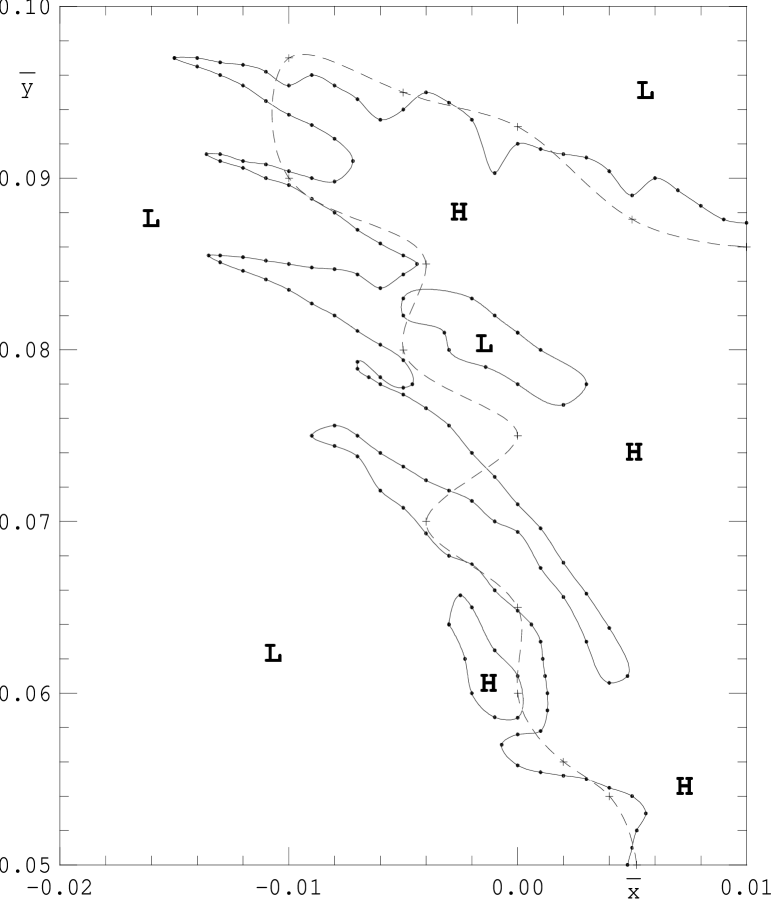
Figure 3: The contour lines of constant LCN at the value $\lambda=10^{-4}$ for a coarse mesh ($\Delta\overline{x}=\Delta\overline{y}=0.005$, dashed line) and a fine mesh ($\Delta\overline{x}=\Delta\overline{y}=0.001$, solid line). Regions of $\lambda>10^{-4}$ and $\lambda<10^{-4}$ are marked with a H and an L, respectively

Following these considerations, we studied the evolution of the bifurcations of some specific multiplicities from the basic orbits 1a and 1b. We have selected the multiplicities 11 and 29 for three reasons: (I) 11 and 29 are prime numbers, so that there are no families of these multiplicities resulting from lower multiplicity families, except from those with multiplicity one. (ii) The number of bifurcating families is neither small nor great. (iii) There are a lot of orbits of these multiplicities on the various BL’s and FTL’s for $\epsilon=0.560$ and $\eta=0.20$.

The detailed discussion in Appendix A and the examples in Appendix B lead to the conclusion that pairs of families without any direct or indirect connection to a basic orbit of the unperturbed system (e.g. the six pairs appearing in Fig. 4) exist in a 3-D system. This happens mainly for high multiplicities, exactly as one would expect considering the analogous case of irregular families in 2-D systems. It should be noted also that, besides the above mentioned classical case of irregular families, in this work we have found a new kind of irregular families, which we call a double pair, i.e a pair consisting of two single pairs (see Fig. 14 and its discussion in Appendix B).

6 Summary and conclusions

Barbanis and Contopoulos (1995), in studying the distribution of the p.c.’s of the periodic orbits in a well known 3-D model potential with the $\overline{x}-\overline{y}$ plane, have discovered a noteworthy order. Except for a couple of gaps, the p.c.’s of periodic orbits, whose multiplicities form Farey-tree sequences, are arranged along continuous and smooth-looking lines. The p.c.’s along these lines have some fractal properties, arising from the fact that they belong to Farey-tree sequences of various orders. In the present work we tried to study the properties of these lines in association with the values of the LCN’s of the area span by them.

We have found numerical evidence that the contour lines of LCN’s show fractal properties. We have also found numerical evidence that the splitting of initially continuous and smooth-looking BL’s and FTL’s, as well as the ensuing formation of gaps, is not an exception, as was implied in BC. As a rule, it is observed in regions of the $\overline{x}-\overline{y}$ plane characterised by high values of the LCN’s and appears not only in BL’s, but in higher order FTL’s as well.

Since our results are only numerical and involve only a small number of periodic orbits, the above results cannot be considered as firm proof that the distribution of BL’s and FTL’s as well as the contour lines of LCN’s have, beyond any doubt, fractal properties. However we feel that there is enough evidence that the above two geometrical objects (BL’s and FTL’s on the one hand and contour lines on the other) are closely related and that, furthermore, they show strong indications of fractal behaviour. Therefore we think that the study of some selected regions of the $\overline{x}-\overline{y}$ should be done in more detail, by calculating LCN’s in even finer mesh and by comparing the contour lines to higher order FTL’s, in order to establish to a higher level of confidence the fractal nature of both geometrical objects.

As far as irregular periodic orbits are concerned, we have found that the majority of the periodic orbits forming BL’s and FTL’s either bifurcate directly from 1a or 1b or they are connected indirectly with them. However, by considering families of periodic orbits with large multiplicities, we find that some of them do not have any connection with 1a or 1b but they form a pair with another family. In the present work we have encountered also the more complex situation of a double pair, i.e. a pair whose members are pairs too.

Appendix A Search for irregular families; bifurcations from the orbit 1a

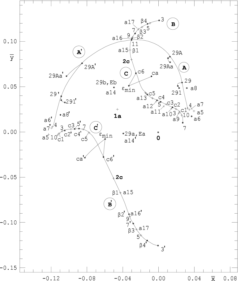
Figure 4: The lines A and A^′, B and B^′, C and C^′ are around orbit 1a. On these lines the p.c.’s of the periodic orbits with multiplicity 29 are depicted, when $\epsilon=0.560$, $\eta=0.20$. The orbits of the corresponding families of the bifurcations from orbit 1a of Table A1 are also given, omitting from each name the prefix 29.

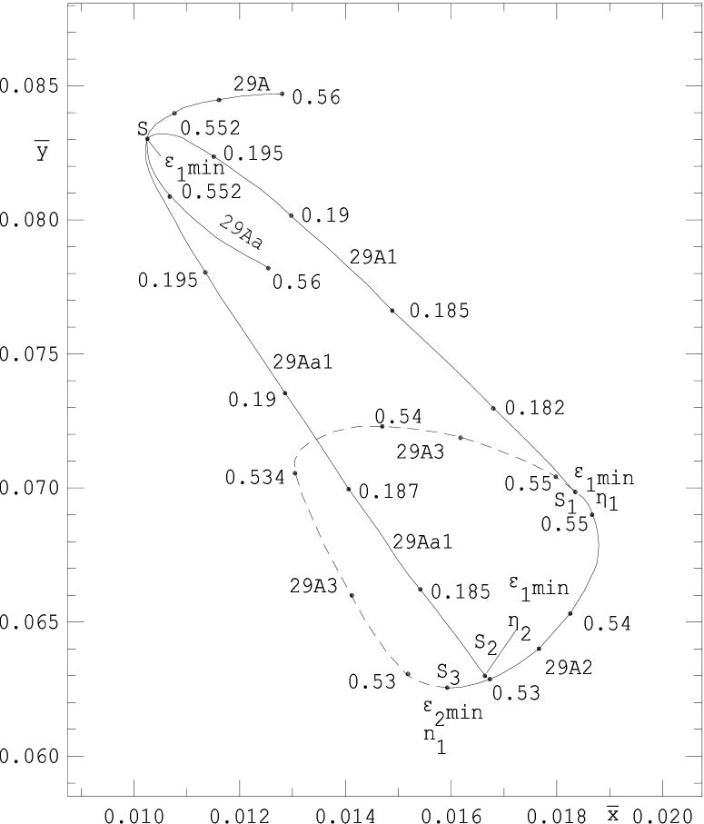
Figure 5: The family 29A forms a pair with the family 29Aa. From the common point S ($\epsilon_{\mathrm{{}_{1}min}},\eta$) emanate the family 29A1 and 29Aa1 by changing $\eta$. The family 29A1 stops at the point S1 ($\epsilon_{\mathrm{{}_{1}min}},\eta_{1}$), while 29Aa1 at the point S2 ($\epsilon_{\mathrm{{}_{1}min}},\eta_{2}$). No continuation of 29Aa1 has been found. On the other hand at the point S1 two other families, i.e. 29A2 and 29A3 emanate with $\eta=\eta_{1}$ and changing $\epsilon$ between $\epsilon_{\mathrm{{}_{1}min}}\leq\epsilon\leq\epsilon_{\mathrm{{}_{2}min}}$. The two families are connected at the point S3 ($\epsilon_{\mathrm{{}_{2}min}},\eta_{1}$). No connection of S3 with 1a has been found.

Tables A1 and A2 give the bifurcating families from the basic family 1a with multiplicities 29 and 11 respectively, when $0\leq\epsilon\leq 0.560$ and $\eta=0.20$. The corresponding bifurcations from 1b are given in Appendix B. The bifurcations from 1a and 1b take place when the index

$$a=-2\cos\left(2\pi R\right)$$ (4)

(where $R$ is the rotation number of the bifurcating orbit) is equal to one of the two indices of the stability, $s$, of the orbits 1a or 1b (Contopoulos & Barbanis 1994). In this way we calculate $\epsilon_{\mathrm{bif}}$, i.e. the value of the parameter $\epsilon$ (for $\eta=0.20$) for which one of the indices of the stability of the orbit 1a or 1b, calculated in quadruple precision, is equal to the index $a$.

Each Table contains the rotation number, $R$, the index $a$, the values of $\epsilon_{\mathrm{bif}}$, the name of each bifurcating family and the way that this family evolves. The name of each bifurcating family from 1a or 1b consists of a letter (a or b) and two numbers. The first number gives the multiplicity, $m$ (11 or 29), and the second the nominator of $R$. For example, 11a7 designates the family with multiplicity 11 which bifurcates from 1a and has $R$ = 7/11. Orbits of families whose nominator of $R$ is odd have two p.c.’s with the ($\overline{x}-\overline{y}$) plane, while those with even nominators have only one. In the case of one p.c. there are two different bifurcating families. We distinguish one of them from the other with an accent to its family name, i.e. 11a6^′.

In Fig. 4 we have drawn the BL’s A and A^′, B and B^′, C and C^′. The origin and the end of these lines are the orbits 4(+) and 11($\cdot$) for A and A^′, 3($\cdot$) and 2c(+) for B, 3^′($\cdot$) and 2c for B^′, 3(+) and 2c(+) for C and C^′. For clarity reasons we omit the prefix 29 from the name of the families in Fig. 4 and Table A1.

Table 1: Bifurcations from 1a with m=29

R	$a$	$\epsilon_{\mathrm{bif}}$	Fam.	Comments
1/29	-1.95324111	0.046714	a1	highly unst.
			a2
2/29	-1.81515084	0.104470		$\gg$
			a2′
3/29	-1.59218613	0.157357	a3	$\gg$
			a4
4/29	-1.29477257	0.207020		$\gg$
			a4′
5/29	-0.93681688	0.253711	a5	see points on
				Fig. 4
			a6
6/29	-0.53505668	0.297548		$\gg$
			a6′
7/29	-0.10827782	0.338633	a7	$\gg$
			a8
8/29	0.32356399	0.377069		$\gg$
			a8′
9/29	0.740277631	0.412949	a9	a9=c1
			a10	a10 = c2
10/29	1.12237413	0.446314
			a10′	a10′ = c2′
11/29	1.45199098	0.477053	a11	a11=c3
			a12	a12=c4
12/29	1.71371435	0.504489
			a12′	a12′=c4′
13/29	1.89530634	0.525074	a13	a13=c5
			a14	a14=29b
14/29	1.98827591	0.5184375
			a14′	a14′=29a
15/29	1.98827591	0.467095	a15	a15=$\beta$1
			a16	a16=$\beta$2
16/29	1.89530634	0.395884
			a16′	a16′=$\beta$2′
17/29	1.71371435	0.310435	a17	a17=$\beta$3
			a18	a18$\rightarrow\beta$4
18/29	1.45199098	0.208203
			a18′	a18′$\rightarrow\beta$4′
19/29	1.12237413	0.085467	a19	a19$\rightarrow$a191

The known orbits of multiplicity 29 on the above lines are:

• On the lines A and A^′ : 29 and 29^′, 29A and 29A^′

• On the lines B and B^′ : $\beta$1, $\beta$2 and $\beta$2^′, $\beta$3, $\beta$4 and $\beta$4^′

• On the lines C and C^′ : c1,c2 and c2^′, c3, c4 and c4^′, c5, c6 and c6^′

• On other FTL lines (not shown here) lie the termination points of the bifurcating families from 1a, with $R$=5/29 to 8/29, namely a5, a6 and a6^′, a7, a8 and a8^′ (see Table A1)

The families of Table A1, which correspond to the first four rotation numbers, become highly unstable as $\epsilon$ increases. This is the reason why the computations were not continued until $\epsilon=0.560$.

The corresponding orbits of the families with $R$=9/29 to 13/29, when $\epsilon=0.560$, are the points c1, c2 and c2^′, c3, c4 and c4^′, c5 of C and C^′ respectively. Similarly, the orbits of the families with $R$=15/29 to 17/29 coincide with the points $\beta$1, $\beta$2 and $\beta$2^′, $\beta$3. The families a14 and a14^′ pass through the point 29b of the spiral Eb and 29a of Ea, respectively. The lines Ea, Eb belong to the spiral structure around 1a as seen in Fig. 1. (see also Fig. 3 in Barbanis 1993).

The families a18 and a18^′ are connected indirectly with the families $\beta$4 and $\beta$4^′ respectively through two other families. A similar example is shown in Fig. 6.

The family a19 bifurcates at $\epsilon_{\mathrm{bif}}=0.085467$ and exists for $\epsilon<\epsilon_{\mathrm{bif}}$ until $\epsilon_{\mathrm{min}}=0.048765$. At this value it is connected to a family which becomes highly unstable at $\epsilon=0.305$.

Each of the remaining orbits 29 and 29A of A , 29^′ and 29A^′ of A^′, c6 of C, c6^′ of C^′ belongs to a family which terminates at some minimum $\epsilon$, where a new family emanates, so that six pairs are formed. E.g. the orbit c6 is the 14th member of the basic sequence C. This family terminates at $\epsilon_{\mathrm{min}}=0.53507$. From this termination point emanates the family ca, which at $\epsilon=0.560$ reaches the point ca on a FTL (see Fig. 4).

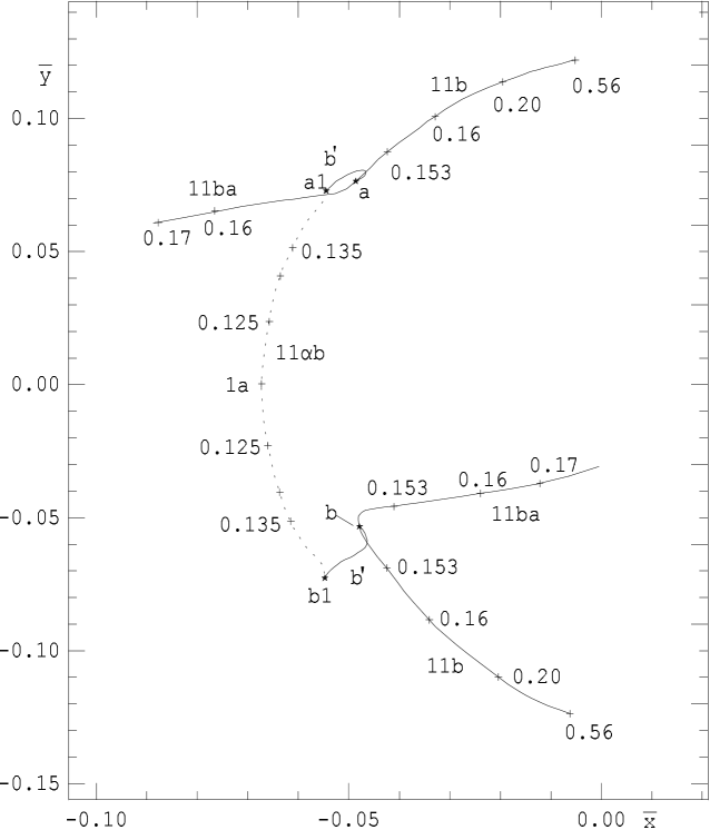
Figure 6: The two branches of the family 11b connect to the branches of the family 11ba, at the points a, b. At these points emanate the branches of the family b^′, which, by changing $\eta$ from 0.20 to 0, reach the points a1, b1. At these points terminate the branches of the family 11ab, which bifurcate from 1a when $\epsilon=0.1227395$, $\eta=0$

Summarizing, the bifurcating families evolve, with respect to $\epsilon$, in the following way:

1. The characteristics of many families move away from the original parent family and, for $\epsilon=0.560$, they cross a BL or a FTL.

2. Some families terminate at a maximum $\epsilon_{\mathrm{max}}$ or a minimum $\epsilon_{\mathrm{min}}$. In this case there are three possibilities:

   • Such a family is connected to another family bifurcating also from the same orbit 1a or 1b and terminating at the same $\epsilon$ (see e.g. 11b2${}^{\prime}\to$11b8^′, Table B1).

   • From the same parent orbit, 1a or 1b, bifurcate two families, one of them terminating at $\epsilon_{\mathrm{max}}$ and the other at $\epsilon_{\mathrm{min}}$. Another family starting at $\epsilon_{\mathrm{min}}$ terminates at $\epsilon_{\mathrm{max}}$ (see Fig. 6). In few cases there are more than one intervening families.

   • From the bifurcating family, which stops at $\epsilon_{\mathrm{max}}$, another family emanates which, for $\epsilon=0.560$, crosses a BL or a FTL (see e.g. 11b3 reaches 11f of F, F^′, Table B1).

3. In bifurcating families with small rotation numbers the computations stop sooner than $\epsilon=0.560$, because the orbits of these families become extremely unstable.

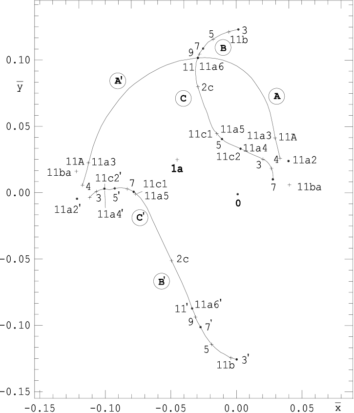
Figure 7: The p.c.’s of the periodic orbits with m=11 are illustrated with the corresponding bifurcating families from 1a. All the orbits on the BL’s are connected directly with 1a, except of 11b, forming a pair with 11ba which is connected indirectly with 1a (see Fig 6)

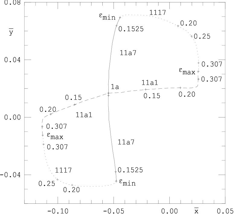
Figure 8: The two branches of the bifurcating families 11a1 and 11a7 from 1a stop at $\epsilon_{\mathrm{max}}=0.3099459$ and $\epsilon_{\mathrm{min}}=0.1522655$ respectively. The family 1117 connects these families.

Some pairs of families that are connected at some $\epsilon_{\mathrm{min}}$ have no direct connection with 1a. The question is: Is there some other family bifurcating from 1a, for some pair of values of $\epsilon$ and $\eta$, which passes through the point from which emanates the pair when $\epsilon=0.560$ and $\eta=0.20$ ?

Fig. 5 represents the pair of 29A and 29Aa; their common point, S, corresponds to $\epsilon_{\mathrm{{}_{1}min}}=0.5504835$, $\eta=0.20$. Keeping $\epsilon=\epsilon_{\mathrm{{}_{1}min}}=const$ and varying $\eta$ we find two other families, 29A1 and 29Aa1, emanating from the common point S. The family 29A1 stops at the point, S1, corresponding to minimum $\eta_{1}=0.181232$, while the family 29Aa1 stops at S2 when $\eta_{2}=0.184350$. All efforts to find a continuation of 29Aa1 were unsuccessful. On the contrary, from the point S1 emanate the families 29A2 and 29A3 for $\eta=\eta_{1}=const$ and $\epsilon$ varying from the value $\epsilon_{\mathrm{{}_{1}min}}$ to $\epsilon_{\mathrm{{}_{2}min}}=0.52840725$, where the two families terminate at the common point S3. No connection of S3 to 1a has been found.

In the case of multiplicity 11 we find that all orbits connect, directly or indirectly, to 1a, except for orbit 11b with two p.c.’s (Fig. 7). This orbit is a Farey tree orbit on the lines B and B^′ between the basic members 3($\cdot$) and 5(+). The two branches of family 11b stop at $\epsilon_{\mathrm{{}_{1}min}}=0.15204035$, $\eta=0.20$ at the two p.c.’s a, b (Fig. 6). From these points emanates the family 11ba which, for $\epsilon=0.560$, passes through points 11ba (see Fig. 7). The two families form a pair with no direct connection to 1a. However, there is an indirect connection to 1a. In fact, starting from the common points a and b with constant $\epsilon=\epsilon_{\mathrm{{}_{1}min}}$ and diminishing $\eta$ from $\eta=0.20$ to $\eta=0$, we reach points a1 and b1. Continuing this family, keeping $\eta=0$ and reducing now $\epsilon$ until the value $\epsilon_{\mathrm{bif}}=0.1227395$, we find that the new family 11ab bifurcates from 1a. Therefore, families 11b and 11ba do not form a pair of irregular families, because this pair is connected indirectly to 1a.

Since our results are numerical, it should be useful to confirm them through further work for the following two reasons:

• The search for bifurcations from 1a and 1b with multiplicity 29 has been confined within the interval $0<\epsilon<0.560$ and $\eta=0.20$ only. One may argue that, although highly improbable, bifurcations for $\epsilon>0.560$ may play the role of connecting bridges of the pairs, considered here as irregular families, to orbits 1a or 1b.

• Following the above argument as well as for reasons of completeness, it would be desirable to find also the bifurcations of 1a and 1b for $\epsilon=0.560$ and $\eta\geq 0$.

Table A2 shows the bifurcations of the orbits with multiplicity m=11 from 1a when $0\leq\epsilon\leq 0.560$, $\eta=0.20$.

On the lines of Fig. 7 we represent the known orbits with m=11, when $\epsilon=0.560$, $\eta=0.20$. These orbits are:

Table 2: Bifurcations from 1a with m=11

R	$a$	$\epsilon_{\mathrm{bif}}$	Fam.	Comments
1/11	-1.68250707	0.138524	11a1	11a1$\rightarrow$11a7
			11a2	point 11a2
2/11	-0.83083003	0.265946
			11a2′	point 11a2′
3/11	0.28462968	0.373682	11a3	11a3=11A of A, A′
			11a4	11a4=11c2 of C
4/11	1.30972147	0.463427
			11a4′	11a4′=11c2′ of C′
5/11	1.91898595	0.527056	11a5	11a5=11c1 of C, C′
			11a6	11a6=11 of B & A
6/11	1.91898595	0.409869
			11a6′	11a6′=11′ of B′
7/11	1.30972147	0.155080	11a7	11a7$\rightarrow$11a1

• On A and A^′ : 11 (also on B), 11A

• On B and B^′ : 11 (also on A) and 11^′, 11b

• On C and C^′ : 11c1, 11c2 and 11c2^′

• On other lines (not showing) 11a2 and 11a2^′, 11ba

The bifurcations of Table A2 are related to the above orbits as follows.

Family 11a1 is connected to family 11a7 through another family 1117, as shown in Fig. 8. Family 11a1 terminates at $\epsilon_{\mathrm{max}}=0.3099459$. Family 11a7 exists for $\epsilon\leq\epsilon_{\mathrm{bif}}$ and terminates at $\epsilon_{\mathrm{min}}=0.1522655$. Family 1117 starts at $\epsilon_{\mathrm{min}}$ and terminates at $\epsilon_{\mathrm{max}}$.

For $\epsilon=0.560$, $\eta=0.20$ the following families pass through the points illustrated in Fig. 7

• Family 11a2 passes though point 11a2, lying on a FTL (not shown). Similarly 11a2^′ passes through 11a2^′

• Family 11a3 passes through point 11A on A and A^′.

• Family 11a4 reaches point 11c2 on C, while 11a4^′ reaches point 11c2^′ on C^′.

• Family 11a5 reaches points 11c1 on C and C^′

• Family 11a6 passes through the cross point 11 of B and A, while 11a6^′ reaches point 11^′ on B^′.

Families which start at points 11b on B and B^′ and 11ba form a pair when $\epsilon=0.15204035$, $\eta=0.20$. This pair has an indirect connection to 1a, as illustrated in Fig. 6.

Appendix B Search for irregular families; bifurcations from the orbit 1b

Table B1 gives the bifurcations with multiplicity m=11 from 1b. Families with $R=4/11$ to $7/11,9/11$ and $10/11$ are not included, because the corresponding values of $a$ are outside the interval of the present study of $0<\epsilon\leq 0.560$ and $\eta=0.20$.

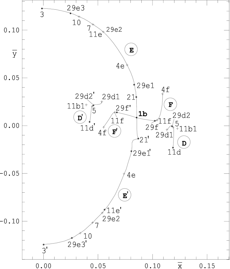
Figure 9: The basic lines E and E^′, F and F^′ cross each other at the periodic orbit 1b, while D and D^′ lie close to 1b. On these lines we show some basic orbits with small multiplicities and the p.c.’s of the periodic orbits with m=11 and m=29.

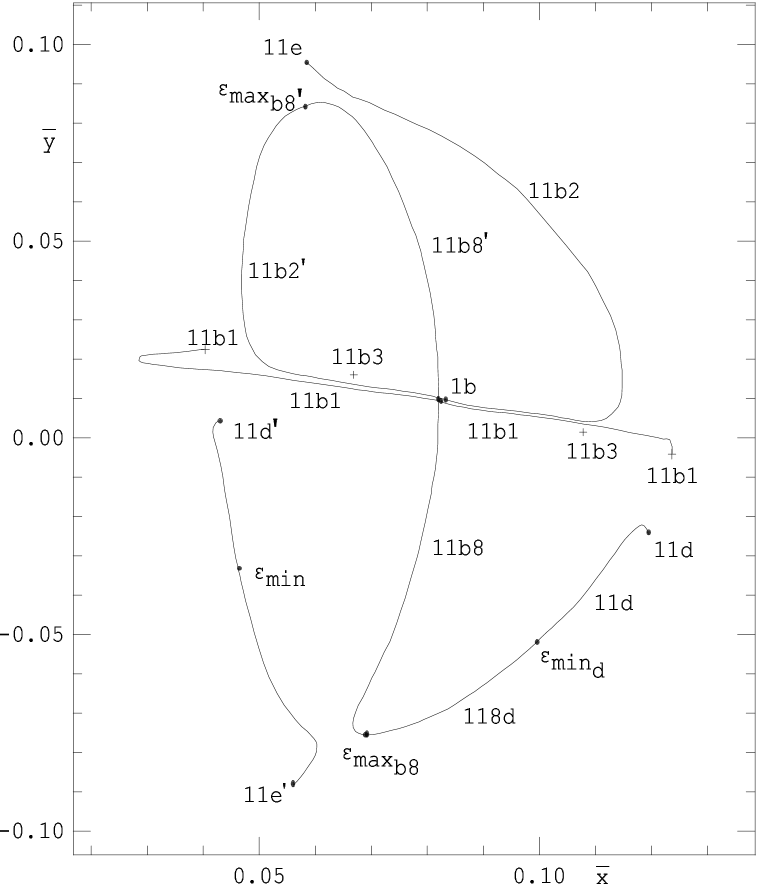
Figure 10: Location of the characteristics of the bifurcating families of Table B1 parametrized by $\epsilon$ ($\eta=0.20$) until $\epsilon=0.560$. Only the last points of family 11b3 are given. The pair of the families 11e^′ and 11d^′ which start through the corresponding orbits on E^′ and D^′ s also shown. Family 11b8 is connected to 11d through the intervening family 118d.

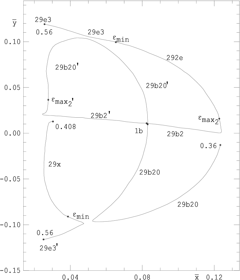
Figure 11: The bifurcating family 29b2^′ is connected to 29b20^′. Families 29b2 and 29e3, corresponding to point 29e3 on E, are connected indirectly through family 292e. Family 29b20 becomes highly unstable at $\epsilon=0.360$. Family 29e3^′ forms a pair with 29x.

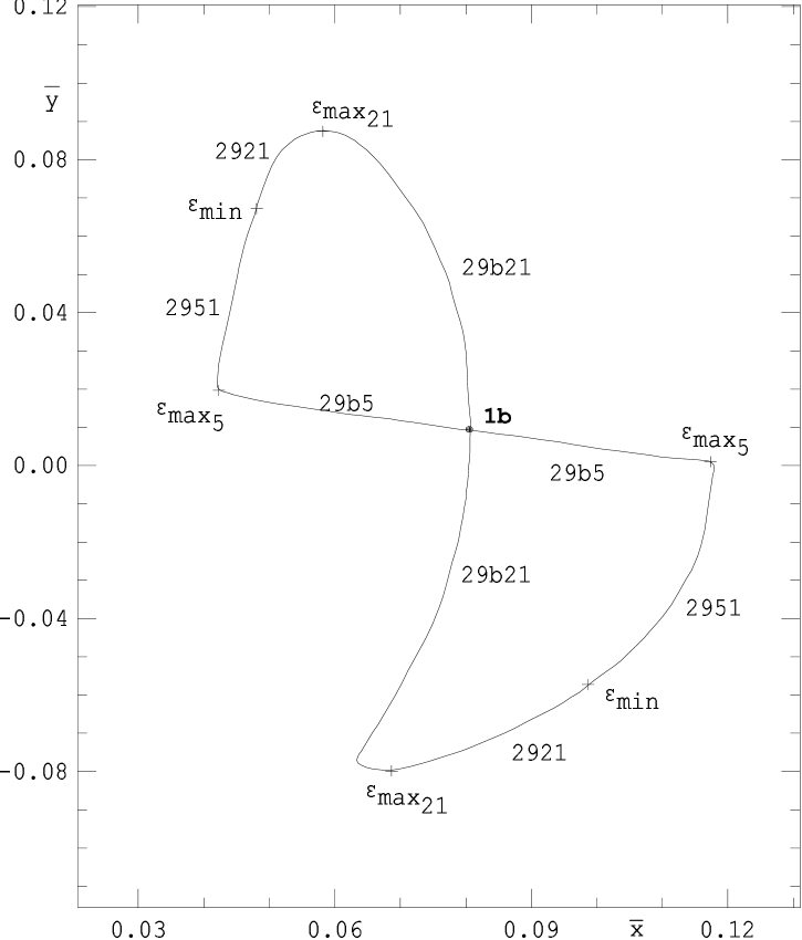
Figure 12: The two branches of the bifurcating families 29b5 and 29b21 are connected through the intervening families 2951 and 2921.

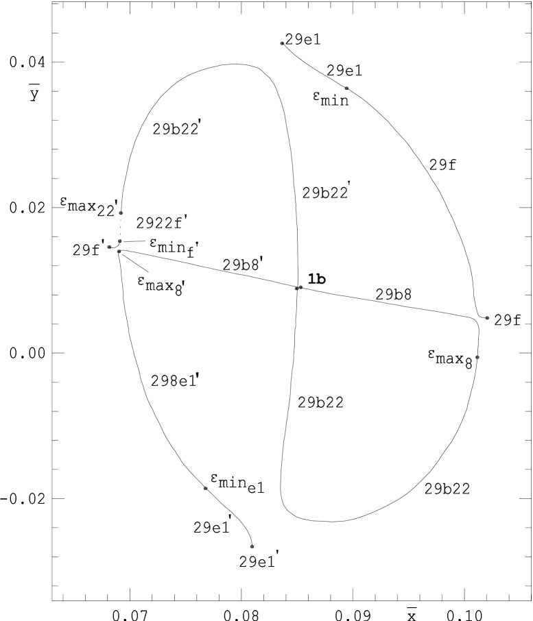
Figure 13: The direct connection of 29b8 to 29b22 as well as the indirect connections of 29b22^′ to 29f^′ through family 2922f^′ and of 29b8^′ to 29e1^′ through family 298e1^′ are illustrated. Families 29e1 and 29f, starting from points 29e1 on E and 29f on F respectively, form a pair which has no obvious connection to 1b.

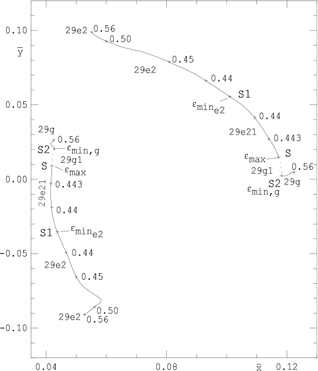
Figure 14: Two pairs of families are connected at the common point S. The first pair, consisting of families 29e2 and 29e21, has as common point S1. The second pair of the families 29g and 29g1 is connected at S2.

Table 3: Bifurcations from 1b with m=11

R	$a$	$\epsilon_{\mathrm{bif}}$	Fam.	Comments
1/11	-1.68250707	0.168452	11b1	11b1=11b1
			11b2	11b2 = 11e of E
2/11	-0.83083003	0.344563
			11b2′	11b2′ $\to$ 11b8′
3/11	0.28462968	0.525391	11b3	11b3=11f of F, F′
			11b8	11b8$\rightarrow$11d of D
8/11	0.28462968	0.290248
			11b8′	11b8′ $\to$ 11b2′

Table 4: Bifurcations from 1b with m=29

R	$a$	$\epsilon_{\mathrm{bif}}$	Fam.	Comments
1/29	-1.95324111	0.063890	29b1	highly unst.
			29b2	29b2$\rightarrow$29e3
2/29	-1.81515084	0.127362
			29b2′	29b2${}^{\prime}\to$29b20′
3/29	-1.59218613	0.192211	29b3	highly unst.
			29b4
4/29	-1.29477257	0.258516		$\gg$
			29b4′
5/29	-0.93681688	0.326001	29b5	29b5$\rightarrow$29b21
			29b6	29b6 = 29d2
6/29	-0.53505668	0.394292
			29b6′	29b6′ = 29d2′
7/29	-0.10827782	0.462973	29b7	29b7 = 29d1
			29b8	29b8$\rightarrow$29b22
8/29	0.32356399	0.531620
			29b8′	29b8${}^{\prime}\rightarrow$29e1′
9/29	0.74027631	$\epsilon_{\mathrm{bif}}$$>$$0.56$
			29b20	29b20 stops
20/29	0.74027631	0.078653
			29b20′	29b20${}^{\prime}\to$29b2′
21/29	0.32356399	0.270218	29b21	29b21$\rightarrow$29b5
			29b22	29b22$\rightarrow$29b28
22/29	-0.10827782	0.516148
			29b22′	29b22′ $\rightarrow$29f′

Fig. 9 depicts the BL’s E and E^′, F and F^′, D and D^′ and the places of the orbits with m=11 and m=29 when $\epsilon=0.560,\eta=0.20$.

The known orbits on these lines are:

• m=11

  • On E and E^′ : 11e , 11e^′

  • On F on F^′ : 11f

  • On D and D^′ : 11d , 11d^′d

• m=29

  • On E and E^′ : 29e1, 29e1^′, 29e2, 29e3, 29e3^′

  • On F and F^′ : 29f, 29f^′

  • On D and D^′ : 29d1, 29d2, 29d2^′

Fig. 10 depicts the characteristics of the families in Table B1, except for family 11b3, because its characteristic is very close to that of family 11b1. Family 11b1 reaches points 11b1 when $\epsilon=0.560$, while family 11b3 reaches the two points 11f of F, F^′.

Family 11b2 passes through point 11e of E. Family 11b2^′ reaches $\epsilon_{\mathrm{max_{b8^{\prime}}}}=0.46578405$, where it is connected to family 11b8^′. Family 11b8 reaches $\epsilon_{\mathrm{max_{b8}}}=0.4622105$, where family 118d emanates. This family connects 11b8 to 11d, which starts at $\epsilon_{\mathrm{min_{d}}}=0.443468$ and, when $\epsilon=0.560$, it reaches point 11d lying on D.

Family 11d^′ terminates at $\epsilon_{\mathrm{min}}=0.443836$, where it joins family 11e^′, which for $\epsilon=0.560$ passes through point 11e^′ of E^′ (Fig. 10). Families 11e^′ and 11d^′ form a pair, not having any obvious connection to the basic orbit 1b.

Table B2 shows the bifurcating families with multiplicities m=29 from 1b. As we mentioned before, the computation of orbits with small $R$, i.e. $R$ = 1/29, 3/29 and 4/29, stops before $\epsilon=0.560$ because these orbits become highly unstable.

Fig. 11 shows the indirect connection of family 29b2 to the family 29e3, starting from orbit 29e3 on E. Family 29b2 terminates at $\epsilon_{\mathrm{max_{2}}}=0.3339236$, while family 29e3 at $\epsilon_{\mathrm{min}}=0.2491375$. The family connecting 29b2 and 29e3 is 292e.

Family 29b2^′ is connected to 29b20^′ at $\epsilon_{\mathrm{max_{2^{\prime}}}}=0.3334738$. On the other hand family 29b20 stops at $\epsilon=0.360$. Family 29e3^′, starting from point 29e3^′ on E^′, reaches $\epsilon_{\mathrm{min}}=0.2491375$, where family 29x emanates. The computation of 29x stops at $\epsilon=0.408$, $\eta=0.20$.

Fig. 12 shows the connection of the branches of families 29b5 and 29b21 through two other families, i.e. 2951 and 2921. Families 29b5 and 29b21 reach $\epsilon_{\mathrm{max_{5}}}=0.44357242$ and $\epsilon_{\mathrm{max_{21}}}=0.4545552$ respectively. Families 2951 and 2921, which are connected at $\epsilon_{\mathrm{min}}=0.4394852$, start, respectively, in these points.

For $\epsilon=0.560$ family 29b6 reaches point 29d2 of the FTL sequence 5(+), ….29d2($\cdot$), 24(+), 19($\cdot$), 14(+), 9($\cdot$) on D, while 29b6^′ is going through point 29d2^′ on D^′ (Fig. 9). Similarly for $\epsilon=0.560$ family 29b7 reaches points 29d1 of the basic sequence D and D^′, namely the sequence with first member the orbit 5(+) and increment 4.

Family 29b8 is connected to 29b22 at $\epsilon_{\mathrm{max_{8}}}=0.55711905$ (Fig. 13). Family 29b8^′ is connected indirectly to 29e1^′, which passes through point 29e1^′ of E^′ when $\epsilon=0.560$. The intervening family 298e1^′ starts at $\epsilon_{\mathrm{min_{e1}}}=0.5520015$ where 29e1^′ stops and meets 29b8^′ at its $\epsilon_{\mathrm{max_{8^{\prime}}}}=0.556970$. Family 29b22^′ continues until $\epsilon_{\mathrm{max_{22^{\prime}}}}=0.55712395$, where family 2922f^′ emanates. This family connects 29b22^′ to family 29f^′. Family 29f^′ starts from orbit 29f^′ on F^′ when $\epsilon=0.560$ and stops at $\epsilon_{\mathrm{min_{f^{\prime}}}}=0.557062675$.

Families 29e1 and 29f, going through points 29e1 on E and 29f on F respectively, form a pair connecting at $\epsilon_{\mathrm{min}}=0.5520015$.

The two branches of family 29e2, which start from points 29e2 on E and E^′ when $\epsilon=0.560$, parametrized by $\epsilon$ ($\eta=0.20$) stop at point S1 when $\epsilon_{\mathrm{min_{e2}}}=0.43790$ (Fig. 14). A new family 29e21 emanates here and terminates at point S when $\epsilon_{\mathrm{max}}=0.4437953$. This pair is connected to another pair which is formed by two families having two branches also. The first family of this pair starts at $\epsilon=0.560$ and $\eta=0.20$ from points 29g, lying on FTL’s and terminates at point S2, when $\epsilon_{\mathrm{min,g}}=0.4435759$. At this point emanates the second family 29g1 of this pair. This family terminates at S together with 29e21. Such a double pair, having no connection to an orbit of the unperturbed system, is noticed for the first time.

References

- (1) Aubry, S., 1978 In : Solitons and condensed matter physics, Bishop, A.R., Schneider, T. (eds.), Springer, Berlin, p. 264
- (2) Avnir, D., Biham, O., Lidar, D., Malcai, O., 1998, Sci 279, 39
- (3) Barbanis, B., 1986, Celest. Mech. 39, 345
- (4) Barbanis, B., 1993, Celest. Mech. Dyn. Astron. 55, 87
- (5) Barbanis, B., 1996, In: Proceedings of the 2nd Hellenic Astronomical Conference, Contadakis M.E., Hadjidemetriou J.D., Mavridis L.N., Seiradakis J.H. (eds.), P. Ziti & Co, Thessaloniki, p. 520-525
- (6) Barbanis, B., Contopoulos, G., 1995, A & A 294, 33 (BC)
- (7) BenKadda, S., Kassibrakis, S., White, R.B. and Zaslavsky, G.M., 1997, Phys. Rev. E 55, 4909
- (8) Contopoulos, G., 1970, AJ 75, 96
- (9) Contopoulos, G., Barbanis, B., 1989, A & A 222, 329
- (10) Contopoulos, G., Barbanis, B., 1994, Celest. Mech. Dyn. Astron. 59, 279
- (11) Efthymiopoulos, C., Contopoulos, G., Voglis, N., Dvorak, R., 1997, J. Phys. A: Math. Gen., 30, 8167
- (12) Gaspard, P., Baras, F., 1995, Phys. Rev. E 51, 5332
- (13) Magnenat, P., 1982, Celest. Mech. 28, 319
- (14) Niven, I., Zuckerman, H., 1960, An Introduction to the Theory of Numbers, Wiley, New York
- (15) Percival, I.C. 1979, In: Non-linear dynamics and the beam-beam interaction, Month M. and Herrera J.C. (eds.), Am. Inst. Phys. Conf. Proc. 57, 302
- (16) Shlesinger, M.F., Zaslavsky, G.M., Klafter, J., 1993, Nature 363, 31
- (17) Tsiganis, K., Anastasiadis, A., Varvoglis, H., 1998, (preprint)
- (18) Varvoglis, H., Anastasiadis, A., 1996, AJ 111, 1718
- (19) Varvoglis, H., Vozikis, Ch., Barbanis, B., 1997, In: The Dynamical Behaviour of Our Planetary System, Henrard J., Dvorak R. (eds.), Kluwer, Dordrecht
- (20) West, B.J., Deering, W., 1994, Phys. Rep 246, 1
- (21) Zaslavsky, G.M., 1994, Physica D 76, 110