From template analysis
to generating partitions II:
Characterization of the symbolic encodings

Abstract

We give numerical evidence of the validity of a previously described algorithm for constructing symbolic encodings of chaotic attractors from a template analysis. We verify that the different solutions that can be found are dynamically equivalent, and that our approach yields results that are consistent with those obtained from methods based on homoclinic tangencies. This is further confirmed by verifying directly that the computed partitions are generating to a high degree of accuracy, and that they can be used to estimate precisely the metric entropy. It is also shown that the correct number of symbols needed to describe the dynamics is naturally provided, and that a compact parameterization of a partition can easily be determined, which makes our algorithm suitable for applications such as real-time encoding.

1 Introduction

In the first part of this work [1], we have presented an algorithm to construct symbolic encodings of a chaotic attractor, which follows the approach proposed in [2]. This algorithm utilizes template analysis [3, 4, 5, 6, 7] to extract symbolic dynamical information from the topological invariants of a set of unstable periodic orbits (UPO) embedded in the attractor.

Template analysis has its roots in the observation that the topological organization of unstable periodic orbits of a three-dimensional hyperbolic flow can be studied in a systematic way [8, 9]. More precisely, there exists a branched two-dimensional manifold, a template, on which all the unstable periodic orbits of such a flow can be laid without modifying their knot-theoretic invariants. The structure of the template thus describes concisely the global organization of the flow.

Because periodic orbits cannot intersect themselves when a control parameter is varied, a set of UPO embedded in a three-dimensional chaotic attractor can be tracked to a regime where the system is hyperbolic without modifying their invariants. In the hyperbolic case, there is a natural coding for periodic orbits: their symbolic names are obtained by listing which branches are successively visited by their projections on the template. It is thus only natural to extend this coding to experimental orbits by requiring that each UPO is assigned the symbolic name of one of the template orbits that has the same topological invariants. This correspondence is one-to-one for a large number of low-period orbits.

Once the possible symbolic names for each detected UPO have been identified in this way, this information must be combined with the knowledge of the position of periodic points in a section plane to construct a generating partition of the latter. In our algorithm, partitions are parameterized by a set of periodic points associated with given symbols, called reference points. To represent an arbitrary trajectory by a symbolic sequence, each intersection with the section plane is encoded by the symbol attached to the closest reference point. Starting from an initial partition based on a small set of low-period orbits (for example a period-$1$ and a period-$2$ orbits), our method progressively refines this partition by inserting higher-period orbits in it while preserving the simplicity of its structure.

The main result of [1] is that this method allows one to obtain high-resolution partitions that have a simple structure, yet which are such that the topological invariants of each detected periodic orbit can be directly read from the symbolic name it has been assigned. That this is at all possible is by itself a strong indication of the validity of the approach. Indeed, we had successfully analyzed a set of more than 1500 orbits, whose intertwining was described by several millions of integers. Preserving the topological consistency of the partition in such a case is by no means trivial. As a matter of fact, we have observed that our algorithm quickly concludes that no consistent solution can be obtained when fed with some arbitrarily chosen initial partitions, or when the input value of a single invariant is purposely modified. This can be because no simple template can be found or because it becomes at some point impossible to make the encoding continuous (such that neighboring points are associated with close symbolic sequences). To be fully convinced of the validity of this approach, however, additional verifications have to be carried out. The aim of this paper is to provide such evidence.

A first test is related to the internal consistency of the algorithm. As different initial partitions lead to different final partitions, we must verify that the latter describe the same dynamics. Returning to the test partition we had obtained in [1], we show in Sec. 3 that this is indeed the case: the partitions that are obtained from the simplest initial partitions that can be built with orbits of periods $1$, $2$, and $4$ are images or preimages of each other.

If partitions obtained by a topological approach are relevant, they should easily identify cases where more than two symbols are needed to describe faithfully the dynamics. We show that this is so in Sec. 4, by considering attractors of the modulated laser equations and of the Duffing equations which display a three-symbol dynamics. The latter example is particularly interesting because a generating partition had previously be obtained for it in Ref. [10], using a method based on homoclinic tangencies [11].

Because the latter method, which is supported by strong numerical evidence [12, 13, 14, 10], is completely orthogonal to ours, a direct comparison of the outputs of both methods is probably the most stringent test one can consider for assessing the validity of the topological approach. As will be seen in Sec. 5, the agreement is excellent: a line of principal homoclinic tangencies is entirely located in the triangles enclosing the border of the partition that was obtained in [1] with a precision of $10^{-4}$. This not only show the equivalence of the two approaches, but also that our algorithm provides reliable error bounds.

This gives an indirect proof of the fact that the partitions we obtain are generating, as this is generally believed to be true for methods based on homoclinic tangencies. Nevertheless, we carry out in Sec. 6 a direct test of this property. It allows us to show that, with an appropriate balance between the numbers of forward and backward symbols, the largest distance between points whose symbolic sequences coincide on a large number of symbols is of the order of the precision with which the partition has been determined. The dependence of this distance with respect to the number of coinciding symbols also indicates that even partitions determined with a relatively low precision suffice to characterize precisely the symbolic dynamics of a chaotic attractor.

In Sec. 7, we compare estimates of the metric entropy obtained (i) from a Lyapunov exponent calculation and (ii) from probabilities of symbol sequences computed from a partition. Again, we find an excellent agreement. For reference, we also characterize the symbolic dynamics of the attractors we have considered in this work by giving for each of them the list of irreducible forbidden words.

Finally, we discuss in Sec 8 how to provide a compact description of a partition by reducing as much as possible the number of periodic points parameterizing it. Last, we conclude by discussing possible extensions and applications of our work.

2 Notations

We first briefly recall the notations that have been defined in [1]. The input data fed to the algorithm is a set $\mathcal{O}$ of $m$ periodic orbits $O_{i}$, whose intersections with a section plane are noted $O_{i}^{j}$, $j=1,\ldots,p_{i}$. From the topological invariants of these orbits, a set of possible symbolic names $\mathcal{N}_{k}(O_{i})$ is first determined. These names are written inside brackets (e.g., $\mathcal{N}(O_{2})=\langle 01\rangle$), to distinguish them from symbolic names of periodic points, which are written using overlined strings (e.g., $N(O_{2}^{1})=\overline{01}$). Indeed, different cyclic permutations of a given name represent the same periodic orbit, but different periodic points.

A partition $\Gamma$ of a section plane divides it in disjoint regions $\Delta_{i}(\Gamma)$, $i=1,\ldots,n$. The symbolic name $N_{\Gamma}(O_{i})$ assigned by a partition $\Gamma$ to a periodic orbit $O_{i}$ is defined as being the one assigned to its first periodic point: $N_{\Gamma}(O_{i})=N_{\Gamma}(O_{i}^{1})=\overline{s_{1}\ldots s_{p_{i}}}$, which is such that $O_{i}^{k}\in\Delta_{s_{k}}(\Gamma)$.

In [1], we had obtained two partitions of an attractor of the modulated laser equations. The first was computed from a set of periodic orbits providing a uniform cover of a Poincaré section of the attractor, with a resolution of $10^{-3}$ (in units of the attractor width), and will be hereafter noted $\Gamma_{a}^{f}$. This partition and the corresponding set of orbits will be used in Sec. 3 to study the relation between partitions computed from different initial partitions, and in Sec. 8 to describe how a compact parameterization of a partition may be obtained.

Using an improved algorithm, and a set of orbits such that the region of the partition border was covered with a high resolution, we had also obtained a second partition whose border line was localized with a precision of $10^{-4}$. This partition will be noted $\Gamma_{h}^{f}$ in the following. It will be used to carry out precise tests related to the equivalence with methods based on homoclinic tangencies (Sec. 5), the closeness to a generating partition (Sec. 6), and estimation of the metric entropy (Sec. 7).

3 Influence of the choice of the initial partition

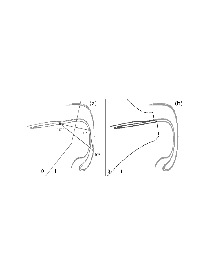
Figure 1: Symbolic encoding of the attractor used as an example in the description of the algorithm in [1]. (a) initial partition, (b) final partition.

We have reproduced in Fig. 1 the partition $\Gamma_{a}^{f}$, with the initial partition $\Gamma_{a}$ that had been used as input. As explained in [1], there is some arbitrariness in the choice of this initial partition. For instance, we know that one point of the period-2 orbit $\langle 01\rangle$ must be assigned the name $\overline{01}$ and the other $\overline{10}$, but this gives two possible choices, which are in principle equivalent: $\{N_{\Gamma}(O_{2}^{1}),N_{\Gamma}(O_{2}^{1})\}$ = $\{\overline{01},\overline{10}\}$ (as in Fig. 1), or $\{N_{\Gamma}(O_{2}^{1}),N_{\Gamma}(O_{2}^{1})\}$ = $\{\overline{10},\overline{01}\}$. Different initial partitions will obviously lead to different final partitions, since the algorithm does not modify the symbols of the reference points after they are inserted in the partition.

We must therefore verify that the solutions obtained using different initial partitions model equivalently the symbolic dynamics of the chaotic attractor, i.e., that the quantities which can be computed using the partition do not depend on the choice of the initial partition, provided the latter is reasonably chosen.

Orbits with a unique topological name are not a problem in this respect. If they were the only orbits to consider, they could in principle be named using any cyclic permutation of their topological name. The first step of the algorithm described in [1] merely ensures that the permutation we choose for each orbit preserves the simplicity of the partition. However, the names of the remaining orbits are determined using not only the topological invariants, but also an intermediate partition. These names might thus vary depending on which initial configuration is chosen, and we must verify that this is not the case.

An initial partition is based on $l$ periodic orbits $O_{i_{1}},O_{i_{2}},\ldots,O_{i_{l}}$ of periods $p_{i_{j}}$, each having a unique topological name $\mathcal{N}(O_{i_{j}})$. Such a partition is completely defined if one specifies for each orbit $O_{i_{j}}$ the symbolic name $N_{\Gamma}(O_{i_{j}})=N_{\Gamma}(O_{i_{j}}^{1})=\sigma^{l_{j}}\mathcal{N}(O_{i_{j}})$ ($0\leq l_{j}<p_{i_{j}}-1$) assigned to its first periodic point. The initial triangulation then consists of the reference points $O_{i_{j}}^{k}$, associated with the symbols corresponding to the chosen cyclic permutations.

In the following, we note $\Gamma_{i_{1},\ldots,i_{n}}^{N_{1},\ldots,N_{l}}$ an initial partition specified in this way, where $N_{j}=N_{\Gamma}(O_{i_{j}}^{1})$. With this notation, $\Gamma_{a}=\Gamma_{1,2}^{\overline{1},\overline{01}}$ represents the initial partition shown in Fig. 1(a) (with $O_{2}^{1}$ being the leftmost periodic point of the $\langle 01\rangle$ orbit).

Since our algorithm is deterministic, the final partition $\Gamma^{f}=\Gamma_{1,\ldots,m}^{N_{1},\ldots,N_{m}}$ that contains all the $m$ periodic orbits detected in the attractor is a functional of the initial partition, which we will note:

$$\Gamma^{f}=A[\Gamma_{i_{1},\ldots,i_{l}}^{N_{1},\ldots,N_{l}}]$$ (1)

Consider now the second possible initial partition based on the period-$1$ and period-$2$ orbits, which is $\Gamma_{b}=\Gamma_{1,2}^{\overline{1},\overline{10}}$ (shown in Fig. 2a). The difference with $\Gamma_{a}$ in Fig. 1a is that the symbols associated with the points of the period-$2$ orbit have been exchanged. Using this new initial partition, we obtain a final partition $\Gamma^{f}_{b}=A[\Gamma_{b}]$ (Fig. 2b), that markedly differs from $\Gamma_{a}^{f}=A[\Gamma_{a}]$ (Fig. 1b).

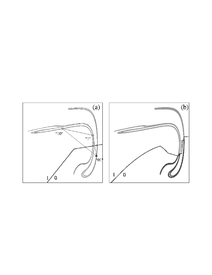
Figure 2: (a) Another possible initial partition using the first two orbits. (b) the resulting partition.

In fact, $\Gamma_{a}^{f}$ and $\Gamma_{b}^{f}$ are related in a very simple way, and describe the same dynamics. Indeed, if we compare for each orbit $O_{i}$ the symbolic names $N_{\Gamma_{a}^{f}}(O_{i})$ and $N_{\Gamma_{b}^{f}}(O_{i})$ assigned by these two partitions, we find that in each case the latter is recovered by shifting the former by one symbol:

$$\forall\,O_{i}\in\mathcal{O},\quad N_{\Gamma^{f}_{b}}(O_{i})=\sigma N_{\Gamma^{f}_{a}}(O_{i})$$ (2)

For example, $N_{\Gamma_{a}^{f}}(O_{3})=\overline{0111}$ and $N_{\Gamma_{b}^{f}}(O_{3})=\overline{1110}$. As a first result, we note that the orbits that had several compatible topological names are identified in the same way by the two final partitions (i.e., up to a cyclic permutation). This seems to indicate that the symbolic names which are singled out in the final partition do not result from an arbitrary choice, but are dynamically relevant.

If we define the action of the shift operator $\sigma$ on a partition as follows (the symbolic names of the orbits parameterizing the partition are all shifted by one symbol):

$$\sigma\Gamma_{i_{1},\ldots,i_{n}}^{N_{1},\ldots,N_{n}}=\Gamma_{i_{1},\ldots,i_{n}}^{\sigma N_{1},\ldots,\sigma N_{n}},$$ (3)

and since relation (2) is verified for every periodic orbit involved in the final partitions, we can write:

$$\Gamma^{f}_{b}=\sigma\Gamma^{f}_{a}$$ (4)

It is trivial to remark that a similar relation holds for the initial partitions:

$$\Gamma_{b}=\Gamma_{1,2}^{\overline{1},\overline{10}}=\sigma\Gamma_{1,2}^{\overline{1},\overline{01}}=\sigma\Gamma_{a}$$ (5)

and thus we have a kind of commutative relation:

$$\Gamma^{f}_{b}=A[\sigma\Gamma_{a}]=\sigma A[\Gamma_{a}]=\sigma\Gamma^{f}_{a}$$ (6)

While relation (6) is formally correct in our particular example, it should not be extrapolated to higher powers of the shift operator, because $\sigma^{2}\Gamma_{a}=\Gamma_{a}$, but $\sigma^{2}\Gamma_{a}^{f}\neq\Gamma_{a}^{f}$. Indeed, for any partition defined with orbits of periods $p_{i}$, we have $\sigma^{l}\Gamma=\Gamma$ where $l$ is the least common multiple of the $p_{i}$. What Eq. (6) essentially indicates is that our algorithm preserves the dynamical relation that exists between initial partitions $\Gamma_{a}$ and $\Gamma_{b}$. This seems to indicate that it converges to the simplest partition that is consistent with the information contained in the initial partition.

Eq. (4) also shows that the two solutions obtained from two different initial conditions are dynamically equivalent, as is best seen by translating Eq. (6) into a relation involving the first return map $f$. Since the shift operator is conjugate to $f$, we have for any detected periodic point $O_{i}^{k}\in\mathcal{P}$:

$$N_{\Gamma^{f}_{b}}(O_{i}^{k})=\sigma N_{\Gamma^{f}_{a}}(O_{i}^{k})=N_{\Gamma^{f}_{a}}(f(O_{i}^{k})),$$ (7)

Consider the set $\Delta_{i}^{\mathcal{P}}({\Gamma})=\Delta_{i}({\Gamma})\cap\mathcal{P}$ of all the detected periodic points lying in region $\Delta_{i}({\Gamma})$ of the partition $\Gamma$. Eq. 7 implies that:

$$\forall i,\quad x\in\Delta_{i}^{\mathcal{P}}({\Gamma_{b}^{f}})\Longleftrightarrow f(x)\in\Delta_{i}^{\mathcal{P}}({\Gamma_{a}^{f}})$$ (8)

and therefore:

$$\forall i,\quad\Delta_{i}^{\mathcal{P}}({\Gamma_{b}^{f}})=f^{-1}\left(\Delta_{i}^{\mathcal{P}}({\Gamma_{a}^{f}})\right)$$ (9)

Because $\Delta_{i}^{\mathcal{P}}({\Gamma_{a}^{f}})$ approximates $\Delta_{i}({\Gamma_{a}^{f}})$ (the periodic points were chosen so as to provide a uniform cover of the attractor), we have:

$$\forall i,\quad\Delta_{i}({\Gamma_{b}^{f}})\approx f^{-1}\left(\Delta_{i}({\Gamma_{a}^{f}})\right)$$ (10)

where $\Delta_{i}(\Gamma)$ should be understood as the intersection of region $i$ with the support of the strange attractor.

Since the image of a partition $\Gamma=\{\Delta_{0}(\Gamma),\Delta_{1}(\Gamma),\ldots\}$ can be defined naturally as $f(\Gamma)=\{f(\Delta_{0}(\Gamma)),f(\Delta_{1}(\Gamma)),\ldots\}$, the relation between partitions $\Gamma_{a}^{f}$ and $\Gamma_{b}^{f}$ can be concisely written as:

$$\Gamma_{b}^{f}\approx f^{-1}\left(\Gamma_{a}^{f}\right)$$ (11)

The reason why the border of $\Gamma_{b}^{f}$ shown in Fig. 2b is not exactly the preimage of the border of $\Gamma_{a}^{f}$ shown in Fig. 1b is that the mediators of the triangles in the latter partition need not be exactly mapped to those of the former. Therefore, if we consider a long chaotic trajectory, and encode it using the two partitions, the obtained symbolic sequences will not be entirely shift-equivalent (whereas this is rigorously true for the periodic orbits used in the partition): there might be discrepancies for points located very close to the border. The degree of equivalence will therefore depend on the precision with which the partition has been determined, i.e., on the size of the triangles enclosing the border of the partition.

To assess the degree of equivalence in our example, we have analyzed a chaotic trajectory of $10^{7}$ iterations, and compared the symbolic sequences obtained with the two partitions (taking into account the shift by one symbol): we found that less than 0.02% of the symbols differed. These observations clearly show that the final partitions obtained using the two initial partitions describe essentially the same dynamics. Note also that to localize the border with a higher precision, it should be possible to use a more sophisticated interpolation scheme where these discrepancies would be taken into account to obtain a solution that is consistent with its images and preimages.

We have examined all initial partitions based on the period-$1$ and period-$2$ orbits. To test further the robustness of our method, we now consider initial partitions based on the four periodic points of the period-$4$ orbit, which will allow us to explore different configurations.

We have four possible initial partitions, each corresponding to a different cyclic permutation of the topological name $\mathcal{N}(O_{3})=\langle 0111\rangle$. In the first two of these partitions, namely $\Gamma_{3}^{\overline{0111}}$ and $\Gamma_{3}^{\overline{1110}}$, the period-$4$ orbit is assigned the same name as in the final partitions $\Gamma_{a}^{f}$ and $\Gamma_{b}^{f}$, respectively. Not surprisingly, we obtain from these two initial configurations the two final partitions that have previously been computed: $A[\Gamma_{3}^{\overline{0111}}]=\Gamma_{a}^{f}=A[\Gamma_{1,2}^{\overline{1},\overline{01}}]$ and $A[\Gamma_{3}^{\overline{1110}}]=\Gamma_{b}^{f}=A[\Gamma_{1,2}^{\overline{1},\overline{10}}]$.

The two other initial partitions, $\Gamma_{3}^{\overline{1101}}$ and $\Gamma_{3}^{\overline{1011}}$, shown in Figs 3a and 4a, yield different partitions which are displayed in Figs 3b and 4b, respectively.

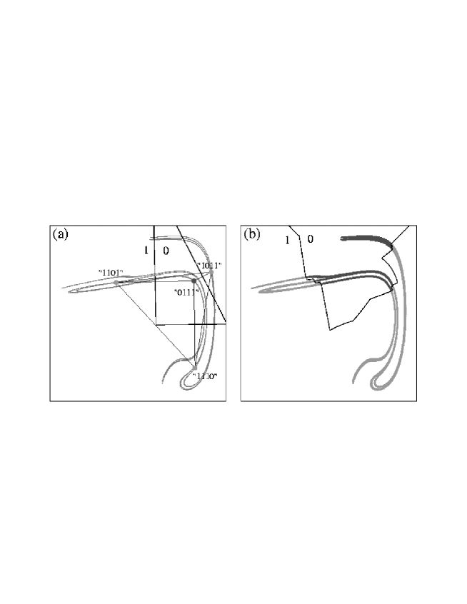
Figure 3: (a) Initial partition $\Gamma_{3}^{\overline{1101}}$ ; (b) the corresponding final partition $A[\Gamma_{3}^{\overline{1101}}]$

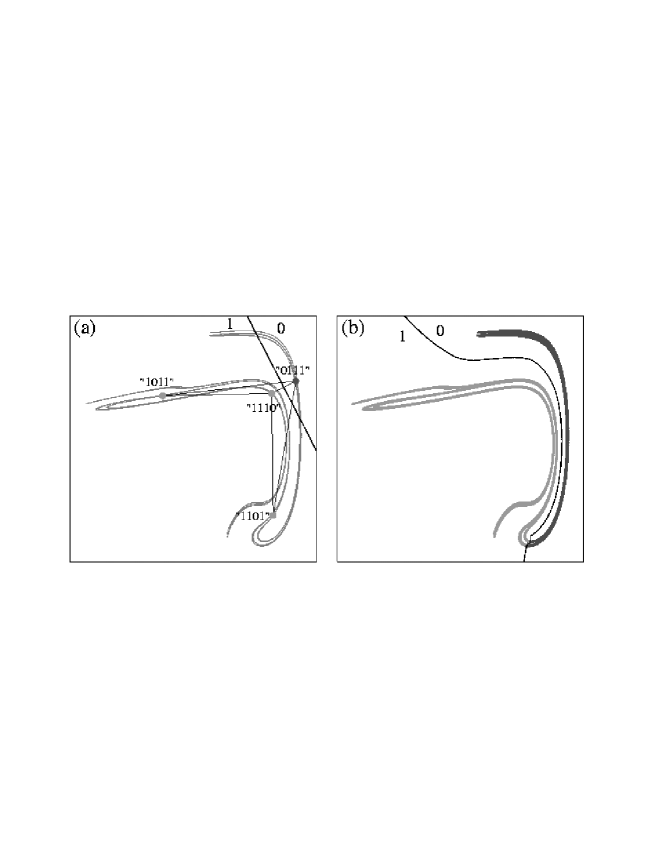
Figure 4: (a) Initial partition $\Gamma_{3}^{\overline{1011}}$ ; (b) the corresponding final partition $A[\Gamma_{3}^{\overline{1011}}]$

Again, these partitions are equivalent to the partition $\Gamma^{f}_{a}$ shown in Fig. 1b, since we have $A[\Gamma_{3}^{\overline{1101}}]=\sigma^{2}\Gamma_{a}^{f}$, and $A[\Gamma_{3}^{\overline{1011}}]=\sigma^{-1}\Gamma_{a}^{f}$.

The four partitions based on the period-$4$ orbit are therefore related by:

$$\sigma^{-2}A[\Gamma_{3}^{\overline{1101}}]=\sigma^{-1}A[\Gamma_{3}^{\overline{1110}}]=A[\Gamma_{3}^{\overline{0111}}]=\sigma A[\Gamma_{3}^{\overline{1011}}]$$ (12)

which translates to:

$$f^{-1}\left(A[\Gamma_{3}^{\overline{1011}}]\right)\approx A[\Gamma_{3}^{\overline{0111}}]\approx f\left(A[\Gamma_{3}^{\overline{1110}}]\right)\approx f^{2}\left(A[\Gamma_{3}^{\overline{1101}}]\right)$$ (13)

which clearly shows that the six simplest initial configurations (two based on $\{O_{1},O_{2}\}$ and four on $O_{3}$) lead to 4 dynamically equivalent final partitions.

However, it should be noted that our algorithm does not converge for every possible initial partition. For example, we have tried the 8 initial partitions based on the 7 periodic points of the set of orbits $\{O_{1},O_{2},O_{3}\}$. Four or them lead to the four final partitions that have already been obtained: these are the initial partitions of the form $\sigma^{k}\Gamma_{1,2,3}^{\overline{1},\overline{01},\overline{0111}}$. The four other initial partitions are of the form $\sigma^{k}\Gamma_{1,2,3}^{\overline{1},\overline{01},\overline{1110}}$: in this case, the algorithm terminates after finding an inconsistency, or yields a partition which has a complicated structure. Note that the latter four initial partitions do not belong to the $\sigma$-orbit of the $\Gamma_{1,2,3}^{\overline{1},\overline{01},\overline{0111}}$ initial partition which leads to the simple solution $\Gamma_{a}^{f}$ shown in Fig. 1b.

This observation and other tests we carried out lead us to conclude that our algorithm is successful whenever the input names defining the initial partition are those assigned by a partition that is one of the first few (pre-) images of the $\Gamma_{a}^{f}$ partition. This supports the idea that there is a natural solution of lowest complexity, and that our algorithm successfully approximates it.

To conclude this section, we note an interesting consequence of the fact that our partitions are parameterized by periodic orbits: forward and backward images of partitions can easily be computed without being faced with the exponential divergence of nearby orbits. To do this, it suffices to shift all the symbolic names given by the final partition by the same amount, and to recompute the border. This property could be useful in chaos-based digital communications: by using the $\sigma^{n}\Gamma_{a}^{f}$ partition, one can predict $n$ iterations in advance the symbol corresponding to the standard partition $\Gamma_{a}^{f}$, allowing for early error recovery.

4 Examples of three-symbol partitions

A difficult problem when trying to construct a symbolic encoding of a given attractor is to determine how many different symbols are needed to describe faithfully the dynamics. If topological entropy cannot be easily computed, metric entropy, which is a lower bound of topological entropy, could be estimated from the greatest Lyapunov exponent. For example, at least $n$ symbols should be used when $\lambda_{1}T>\ln n$, where $T$ is the modulation period. However, there can be situations where the right number of symbols is larger than indicated by the topological entropy because there are many forbidden symbolic sequences.

Besides their robustness, methods based on template analysis have the advantage that the correct number of symbols is automatically obtained from the preliminary template analysis: this is just the number of branches of the simplest template that describes the topological organization of the data.

To illustrate this, we now apply our algorithm to two strange attractors whose symbolic dynamics involve three symbols: an attractor of the modulated laser equations used in [1], but at different parameter values, and an attractor of the Duffing system at the parameters studied in Ref. [10], where a generating partition was determined from the locations of the homoclinic tangencies.

4.1 Symbolic encoding of a spiral modulated laser attractor

Depending on the parameters, the regimes displayed by a chaotic system can have different degrees of complexity: some may correspond to a two-symbol dynamics while the description of other, more chaotic, regimes requires a larger number of symbols.

This is the case of the modulated laser equations whose parameter space is divided in several regions corresponding to different topological organizations, as is common for nonlinear oscillators [15]. To test our algorithm in a more complicated case than the one considered in [1], we have studied an attractor close to the three-branch spiral attractor described in Ref. [16], and whose parameters are the same as in [1], except that $m=0.08125$, $\gamma=1.5\times 10^{-3}$, and $\omega\approx 0.923077\omega_{r}$ where $\omega_{r}=\sqrt{\gamma(A-1)}$ is the relaxation frequency of the laser.

That an analysis of this attractor requires at least three symbols is readily indicated by the fact that it contains four period-$3$ orbits, whereas at most two exist in a two-symbol dynamics. This is confirmed by a template analysis, which shows that the topological structure of this attractor is described by a spiral three-branch template (a.k.a. “Gâteau Roulé”), described by the following template and layering matrices:

$$t^{S}=\left(\begin{array}[c]{ccc}0&0&0\\ 0&1&2\\ 0&2&2\end{array}\right),\quad{l}^{S}=\left(\begin{array}[c]{ccc}0&2&1\end{array}\right)$$ (14)

An illustration of the corresponding three-branch manifold can be found in Fig. 6 of Ref. [16]. The partition shown in Fig. 5 has been obtained using the improved procedure outlined at the end of Ref. [1], and is based on a set of $1250$ orbits of periods up to $32$ which provides a resolution better than $10^{-3}$ in the region of the border. It should be noted that in this case, there is only one initial partition based on the period-$1$ and period-$2$ orbits $\langle 1\rangle$ and $\langle 01\rangle$ that leads to a simple solution, the one which assigns the symbol “0” to the leftmost period-$2$ point. Indeed, the algorithm does not converge if we exchange the symbols of the period-$2$ points. This is due to the template having three branches: exchanging these two periodic points would amount to placing branch “0” between branches “1” and “2” and would violate the requirement of continuity.

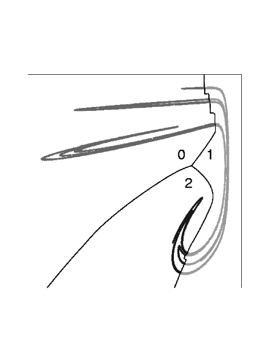
Figure 5: Generating partition for a three-branch spiral attractor of the modulated laser equations.

4.2 Symbolic encoding of a Duffing attractor

The Duffing system

$$\dot{x}=y,\quad\dot{y}=-\delta y+x-x^{3}+\gamma\cos ft$$ (15)

is one of the few three-dimensional flows for which a generating partition has been determined by methods based on homoclinic tangencies [10]. To verify that our approach yields results that agree with these methods, we have therefore applied our procedure to the regime studied in Ref. [10], which corresponds to parameters $\delta=0.25$, $\gamma=0.4$, and $f=1$.

A direct template analysis indicates that the topological structure can be described by the following six-branch matrices:

$$t^{D}=\left(\begin{array}[c]{cccccc}2&2&0&0&0&2\\ 2&1&0&0&0&2\\ 0&0&0&0&0&2\\ 0&0&0&2&2&2\\ 0&0&0&2&1&2\\ 2&2&2&2&2&2\end{array}\right),\quad{l}^{D}=\left(\begin{array}[c]{rrrrrr}0&-1&1&3&2&-2\end{array}\right)$$ (16)

It can be seen that the template matrix in Eq. (16) does not describe a continuous branched manifold because the torsions of two adjacent branches differ by two units. Presumably, these matrices correspond to a part of a larger template. This is however not important, as it turns out that the dynamics of this regime can be studied with only three symbols.

Indeed, as noted in Refs. [10, 15], we can take advantage of a symmetry of the Duffing equations (15) to simplify the analysis, namely the invariance under the transformation $x\rightarrow-x,y\rightarrow-y,\phi\rightarrow\phi+\pi$. This symmetry indicates that the dynamics during the first half-period and during the second half-period are seentially equivalent. As a consequence, the Poincar sections at $\phi=0$ and $\phi=\pi$ are identical modulo an inversion around the origin. We will thus consider the reduced dynamical system, where the integration of Eqs. (15) over half a period is followed by a twist of a half-turn.

If we discard two solutions where torsions of adjacent branches differ by more than one half-turn and which are algebraically equivalent to the solutions presented below [16], we find two possible templates for this reduced system. The first one is described by the matrices:

$$t^{D_{1}}=\left(\begin{array}[c]{ccc}1&2&2\\ 2&2&2\\ 2&2&3\end{array}\right),\quad{l}^{D_{1}}=\left(\begin{array}[c]{rrr}0&-2&-1\end{array}\right)$$ (17)

which correspond to the spiral template described by Eqs. (14) with an additional half-twist and which was identified as a building block for the Duffing template by Gilmore and McCallum [15]. The other one is a S-shaped template, whose matrices are:

$$t^{D_{2}}=\left(\begin{array}[c]{ccc}2&2&2\\ 2&1&2\\ 2&2&2\end{array}\right),\quad{l}^{D_{2}}=\left(\begin{array}[c]{rrr}0&-1&-2\end{array}\right)$$ (18)

These two solutions are algebraically compatible with the topological invariants of the UPO: for each of the two templates, it is possible to find a set of periodic orbits lying on it that has exactly the same invariants as the experimental ones. This means that the spectra of periodic orbits of the two templates have subsets that are isotopic, and that the set of detected orbits in the Duffing attractor belongs to this intersection. Yet, this indeterminacy is intriguing, as the above two solutions have quite different topological structures.

However, there is a clear-cut difference between these two solutions which is unveiled when trying to construct a symbolic encoding. Whereas a partition is easily found using the first template (described by Eqs. (17)), our algorithm quickly stops when the second one is used as input: at some point the current partition is such that some orbits do not any longer have at least one topological name compatible with it. This means that one cannot find a symbolic encoding that is simultaneously continuous in the section plane and reproduces the symbolic dynamics associated with the template (18). We believe that this indicates that only the first solution is dynamically relevant. Thus, although we focus here on the application of template analysis to the construction of symbolic encodings, we see that our algorithm can also be helpful to discriminate algebraic solutions of the template-finding problem.

The partition obtained with template (17) is shown in Fig. 6. It is based on a set of $1326$ periodic orbits of periods up to $36$, providing a cover with a resolution better than $10^{-3}$ in the neighborhood of the border. It is seen to reproduce Fig. 4 of Ref. [10], where the partition had been computed by following lines of homoclinic tangencies. It should be stressed that in our case, this partition is the simplest and most natural solution (obtained from an initial configuration based on the period-1 and period-2 orbits). In contrast with this, it was noted in Ref. [10] that some homoclinic tangencies involved in this partition are not primary, and that heuristic considerations had to be used to select these particular tangencies. This shows that the topological approach provides us with additional information that cannot be obtained from the study of homoclinic tangencies, and is thus a powerful tool for selecting the correct lines of tangencies.

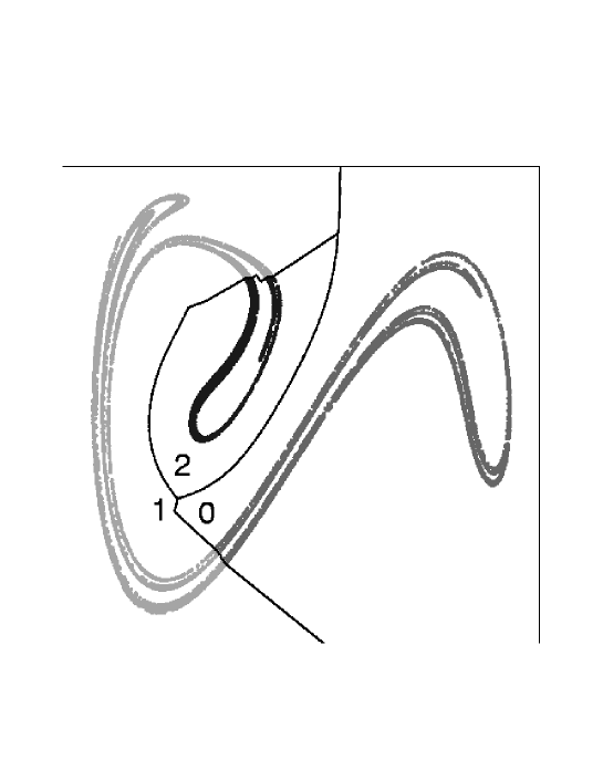
Figure 6: Generating partition obtained for the Duffing attractor.

Although the partition shown in Fig. 6 does not differ to the eye from the partition computed in Ref. [10], we still have to verify precisely that the two approaches still agree at the smallest scales. In particular, we must check whether the error bounds naturally provided by our algorithm are correct: if so, the partition border determined using homoclinic tangencies should be entirely located inside the region where the coding is considered uncertain (i.e., in the circumcircles of the triangles with different symbols, see [1]). We carry out this verification in the next section.

5 Comparison with methods based on homoclinic tangencies

A difficult problem associated with using homoclinic tangencies to construct partitions is that there is a countable infinity of homoclinic tangencies: all the forward and backward images of a homoclinic tangency are themselves homoclinic tangencies. As a consequence, there are homoclinic tangencies everywhere in the attractor (just as the critical point of the logistic map has preimages in every part of the interval).

However, there are homoclinic tangencies that are more relevant for a large-scale characterization of an attractor, because their influence is felt over a wider region: they should be preferably selected to build a partition line. A possible selection criterion proposed in Ref. [10] is that the sum of the curvatures of the stable and unstable manifolds at the tangency should be minimal, because the curvature of the stable (unstable) manifold diverges when following the backward (forward) orbit of a given tangency.

To illustrate the existence of “principal” homoclinic tangencies in the case of the modulated laser equations (as the same parameters as in [1]), we have plotted in Fig. 7 the points (extracted from a sequence of $10^{8}$ iterations) where the angle between the invariant manifolds, computed using the method described in Appendix B of Ref. [17], is smaller than a prescribed value. It is readily seen that there are regions where this angle remains small over a significantly large region of the section plane, whereas no point with a small angle is detected elsewhere (although there are regions with such points everywhere, there are too small to be visited in a reasonable amount of time by a typical trajectory).

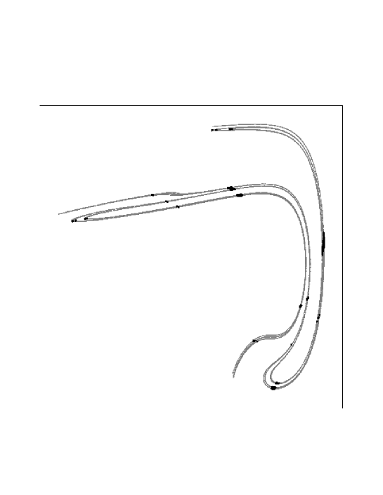
Figure 7: Poincar section of an attractor of the modulated laser equations. The points where the angle between the stable and the unstable manifolds is smaller than 0.1 radians are plotted in black.

A first interesting result is that the wider small-angle regions in Fig. 7 are seen to correspond to some of the partitions that have been obtained in Sec. 3 for different initial configurations. This is obviously related to the fact that these borders have been shown to be images or preimages of each other.

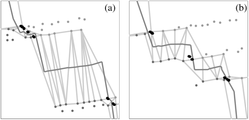
Figure 8: Enlarged views of two neighborhoods of the border line of the high-resolution partition $\Gamma_{h}^{f}$. The size of the two represented squares is $2.5\times 10^{-3}$, in units of the attractor width. Light dots represent periodic points parameterizing the partition. Heavy dots indicate homoclinic tangencies (the angle between the two invariant manifolds at these points is below $2\times 10^{-4}$ radians). The border line and the triangles enclosing it are also represented. The linewidth used to draw the border line is $2.5\times 10^{-5}$.

To make the comparison more precise, we show in Fig. 8 enlarged views of neighborhoods of the border of the high-resolution partition $\Gamma_{h}^{f}$ (see Sec. 2), in which we have indicated the approximate locations of homoclinic tangencies. The agreement is seen to be excellent: all the homoclinic tangencies are located inside the triangles that enclose the border of the partition. This does not only show that the partition line is well approximated by our method, but also that the error bounds it provides strictly hold.

We have also verified this to be true in the case of the spiral laser attractor and of the Duffing attractor which were considered in Sec. 4. Because the latter example is one of the few three-dimensional flows for which a generating partition has been obtained from homoclinic tangencies [10], the equivalent of Fig. 8 for the Duffing attractor is displayed in Fig. 9. The reason why the locations of homoclinic tangencies are better resolved in Fig. 9a than in Fig. 9b is that the same limit angle ($5\times 10^{-4}$ radians) was used in both cases. As the line of homoclinic tangencies shown in Fig. 9b is a principal line, but not the one of Fig. 9a, the region in Fig. 9b where the angle between invariant manifolds is smaller than this value is markedly wider than in Fig. 9a. However, the relatively lower precision in Fig. 9b still allows one to verify that homoclinic tangencies are located inside the triangles enclosing the border of the partition.

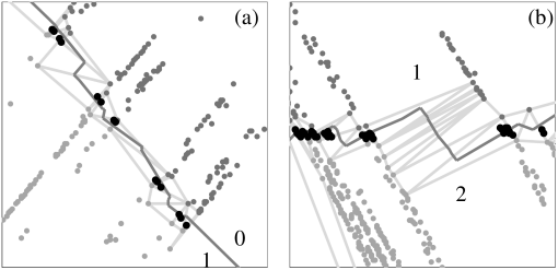
Figure 9: Enlarged views of two neighborhoods of the border line of the partition of the Duffing attractor shown in Fig. 6. Black heavy dots represent points of homoclinic tangency. The widths of the represented squares and of the border line are $10^{-2}$ and $10^{-4}$, respectively. (a) part of the border between $\Delta_{0}$ and $\Delta_{1}$, (b) part of the border between $\Delta_{1}$ and $\Delta_{2}$.

As can be seen in Figs. 8 and 9, the results of this section give strong evidence that algorithms based on template analysis and on the structure of the homoclinic tangencies converge to the same answer. The theoretical tools which these two methods rely on are so utterly different that this agreement is quite fascinating and shows that chaotic dynamics can be studied from multiple points of view. Because of the (at least superficially) complete independence of the two approaches, we believe that this result not only supports the validity of the topological approach, but also provides an additional confirmation of the correctness of methods based on homoclinic tangencies.

Since partitions based on homoclinic tangencies are believed to be generating, this should also be true for the partitions obtained with our algorithm. Nevertheless, in order to make our study complete and to obtain an estimate of the resolutions that would actually be required for practical applications, we carry out in the next section a direct test of this property.

6 Are topological partitions generating?

The defining property of a generating partition is that the trajectories of two different points are encoded with different symbol sequences. In our algorithm, this is by construction enforced for the periodic orbits detected in the strange attractor and utilized in the topological analysis. Nevertheless, it is important to quantify the deviation of the obtained partitions from the ideal case where the mapping from bi-infinite symbolic sequences to chaotic trajectories is well-defined and continuous.

More precisely, let us consider “cylinders”:

$$C(s_{-m}\ldots s_{-1}.s_{0}s_{1}\ldots s_{n-1})=\left\{x\,;s_{\Gamma}(f^{i}(x))=s_{i},i=-m,\ldots,n-1\right\}$$ (19)

which are regions of the Poincaré section of the attractor containing points whose $m$ backward and $n$ forward symbols are identical. A partition $\Gamma$ is generating if and only if:

$$\lim_{n,m\to\infty}\delta_{M}(\Gamma,m,n)=0,\quad\text{with }\delta_{M}(\Gamma,m,n)=\max_{C\in\,\mathcal{C}_{\Gamma}[m,n]}\delta(C)$$ (20)

where $\mathcal{C}_{\Gamma}[m,n]$ is the set of all cylinders with $m$ backward and $n$ forward symbols and $\delta(C)$ is the diameter of a cylinder.

For a given sequence length $l=m+n$, there is a number $n$ of forward symbols that will minimize $\delta_{M}(\Gamma,l-n,n)$. Because backward (resp. forward) symbols specify the position of a point along a segment of the local stable (resp. unstable) manifold, the optimal $n$ and $m$ verify $n\lambda_{1}\approx m\lambda_{2}$, with $\lambda_{1}$ and $\lambda_{2}$ being respectively the positive and negative Lyapunov exponents of the return map.

We can thus characterize how close a partition $\Gamma$ is to a generating partition by the quantities:

$$\rho(\Gamma,l)=\min_{n}\delta_{M}(\Gamma,l-n,n),\quad\rho(\Gamma)=\lim_{l\to\infty}\rho(\Gamma,l)$$ (21)

For a generating partition, $\rho(\Gamma)$ should be zero. If a finite value is obtained, it quantifies the deviation of the partition $\Gamma$ from a generating one.

We have studied the convergence of $\rho(\Gamma,l)$ with increasing $l$ for the high-resolution partition $\Gamma_{h}^{f}$ (see Sec. 2), as shown in Fig. 10. After an approximately logarithmic decrease, $\rho(\Gamma,l)$ is seen to saturate slightly below $3\times 10^{-4}$ of the attractor width. It should be noted however that because $\rho(\Gamma,l)$ can be reliably estimated only if there is a sufficient number of points in the largest cylinder, we did not carry out the computations for $l>70$. Thus, we cannot guarantee that $\rho(\Gamma,70)$ represents the final plateau. Nevertheless, it is consistent with the fact that the border of this partition is localized almost everywhere with a precision better than $10^{-4}$.

Figure 10: Convergence of $\rho(\Gamma,l)$ vs. the total number of symbols $l$. Diameters are expressed in units of the attractor width. For comparison purposes, the dashed line represents the evolution of the geometric average of all cylinder diameters for a given number of symbols (only values for which all cylinder sizes could be reliably estimated are shown). The latter curve is seen to converge to zero much more rapidly. We have verified that it is almost insensitive to the precision with which the border is located.

To illustrate the fact that the saturation value of the quantity (21) provides an estimate of the quality of the partition, we have performed the same test for the logistic map $x_{n+1}=4ax_{n}(1-x_{n})$ at $a=0.955$, where it has roughly the same symbolic dynamics as our sample system (up to length 12, there is only one forbidden sequence, which is “00”). Besides the correct partition, whose border is located at the critical point, we characterized different partitions with borders displaced by a small amount (Fig. 11). As a rule of thumb, $\rho(\Gamma,l)$ appears to saturate at roughly twice the error on the location of the partition border. As this ratio is likely to be larger in the case of a two-dimensional system, the curve in Fig. 10 seems to be consistent with an error on the partition border of the order of $10^{-4}$ of the attractor width.

Figure 11: Equivalent of Fig. 10 for the logistic map. The solid curves represent the evolution of the largest cylinder diameter vs. the number of symbols for the correct partition and for partitions where the border is displaced by a fraction $10^{-4}$, $10^{-3}$, and $10^{-2}$ of the attractor width. These curves can be seen to saturate at a value which is roughly twice the error on the location of the partition border. The dashed line corresponds to the geometric average of cylinder diameters.

A comparison of Figs. 10 and 11 also shows that to reach a given maximal diameter, the two-dimensional case requires roughly twice as many symbols as the one-dimensional one. We attribute this to the fact that two directions are needed to locate a point in the former case. As a result, the convergence of the curve in Fig. 10 is very slow: it takes 31 symbols for the maximal diameter to fall below $0.01$. Since saturation is reached at much smaller scales, this should be a genuine property of the system and not an artifact of our algorithm.

This slow convergence can be traced back to the nonhyperbolicity of the attractor. Near the border, hence near homoclinic tangencies, the stretching rate is very close to 1, and very little information is gained at each iteration of the return map. This has important consequences, as this indicates that it would be pointless to require that the border be localized with a high precision.

Whether we want to characterize the grammar of chaos, i.e., determine the list of forbidden sequences, or use the chaotic system to transmit a digital signal [18, 19], 10–12 symbols should represent a reasonable amount of information. From the curve in Fig. 10, we see that the maximal diameter for 12 symbols is around $0.12$. If error estimates obtained from saturation values can be trusted (Fig. 11), a precision of a few per cent should therefore be sufficient.

In regions of parameter space where the topological entropy is sufficiently large (the number of forbidden symbolic sequences, hence of pruned periodic orbits, should not be too large), such a precision can be easily obtained from a topological analysis of unstable periodic orbits embedded in an experimental chaotic attractor. In fact, a precision of about one per cent has already been achieved for a partition of an attractor observed in a modulated laser [2]. Topological methods for constructing symbolic encodings thus appear to be perfectly suited to the symbolic dynamical characterization of experimental systems, especially given their robustness to noise.

To conclude this section, we note that the above remarks are consistent with the observations reported by Bollt, Lai and Grebogi [20] in their work on noise resistance in chaos-based communication schemes. To prevent noise-induced “bit-flipping”, the trajectory of a chaotic communication device should be kept at a finite distance of the partition border. Enforcing a forbidden zone inside the attractor discards some symbolic sequences and in principle reduces the channel capacity (measured by the topological entropy). The authors of Ref. [20] noted that in fact the latter decreases very slowly when the gap is increased. This is of course due to the near-border cylinders having a large diameter. In contrast with this, the diameters of cylinders in the remaining of the attractor decrease very rapidly with the number of symbols, as is shown by the evolution of the geometric average of the cylinder diameters in Figs. 10 and 11. This ensures that a system can be forced to follow a prescribed symbolic sequence using only tiny perturbations.

A key property of a generating partition is that it can be utilized to estimate various invariant quantities such as metric entropy. In the following section we characterize our partitions by measuring the latter and by giving for each of our sample attractors the list of forbidden sequences.

7 Estimates of metric entropy

There are quantitative measures of chaos that can be recovered both from a study of symbolic dynamics and from a direct analysis of trajectories in phase space. The most important is probably the metric entropy $h_{1}$ which can be defined in symbolic dynamical terms as:

$$h_{1}=\lim_{l\to\infty}h_{1}(l),\quad h_{1}(l)=H(l)-H(l-1),\quad H(l)=-\sum_{S_{l}}p(S_{l})\ln p(S_{l})$$ (22)

where the $S_{l}$ are the allowed symbolic sequences of length $l$, and the $p(S_{l})$ are their probabilities of occurrence in the sequence associated with a typical chaotic orbit. In phase space, a good estimate of $h_{1}$ can be obtained by a standard Lyapunov exponent calculation, since it is conjectured that the metric entropy is equal to the sum of the positive Lyapunov exponents (see, e.g., [21]).

To verify that a partition constructed from a topological analysis of unstable periodic orbits allows one to compute an accurate estimate of the metric entropy, we have thus compared estimates obtained by these two approaches for the regime of the modulated laser system which was studied in [1], using the partition $\Gamma_{h}^{f}$ (see Sec. 2).

First, an estimate of the positive Lyapunov exponent was obtained in the standard way by integrating the linearized equations of motion around a numerical solution over a time interval of $10^{7}$ periods of modulation. This yielded the value $\lambda_{1}\approx 0.3730$.

Then we computed the probabilities $p(S_{l})$ for symbol strings of lengths up to $l_{M}=30$ from a sequence of $10^{8}$ symbols obtained by encoding a chaotic orbit with the partition $\Gamma_{h}^{f}$. To minimize systematic errors due to low-probability strings, we applied to Eq. (22) the finite sample corrections derived by Grassberger [22]. The corresponding estimates of $h_{1}(l)$ are shown in Fig. 12.

Figure 12: Estimates of the metric entropy using finite sample corrections of Eq. 22 vs. string length $l$. The horizontal line indicates the value obtained from Lyapunov exponent calculations and the dashed lines correspond to $\pm$ 1% deviations from this value.

The best estimate is $h_{1}\approx h_{1}(30)=0.374$ which closely agrees with $\lambda_{1}$ as they differ by only $0.3\%$. Furthermore, estimates within 1% of the correct value are obtained for $l>20$. It is however difficult to give precise error bars. Indeed, Eq.(22) systematically overestimates the metric entropy because it does not take into account the forbidden strings of length greater than $l_{M}$. Conversely, the fact that some low-probability sequences may have not been observed can lead to underestimate the entropy.

Furthermore, it should be noted that this test is probably not very sensitive to the quality of the partition: the metric entropy estimate is maximal for a generating partition and thus should remain almost constant when the border of the partition is slightly displaced. Nevertheless, we see it as another check of the validity of our algorithm.

A perhaps more robust characterization of a chaotic regime is to give the list of irreducible forbidden words (IFW) [23], which define the “grammar” of this regime. They are the shortest forbidden symbolic sequences such that every forbidden sequence contains at least one of them, and can be used to compute topological entropy. If we do so for the regime under study, this reveals that it is very close to the crisis where the attractor collides with a period-$3$ orbit [2]: the only forbidden sequence up to period 12 is the “00” string. For reference, we give in Table 1 the list of irreducible forbidden words up to length 17.

Table 1: List of irreducible forbidden words up to length 17 for the partition $\Gamma_{h}^{f}$.

length	irreducible forbidden words
2	$0^{2}$
13	$(01)^{2}(011)^{3}$, $0111(011)^{3}$
15	$(01)^{2}(011)^{2}(01)^{2}0$, $0111(011)^{2}(01)^{2}0$, $(011)^{5}$
17	$(01)^{2}(011)^{2}0101110$, $0111(011)^{2}0101110$,
	$(011)^{4}(01)^{2}0$, $1^{3}01(011)^{4}$, $1^{5}(011)^{4}$

Because the list of irreducible forbidden words is an important characterization of the dynamics, and to allow future comparisons of our results with these obtained from other methods, we also provide in Tables 2 and 3 the list of IFWs for the spiral laser and Duffing attractors studied in Secs. 4.1 and 4.2. In the latter example, note that symbols “0” and “1” should be exchanged to compare the list of IFWs to that of Ref. [10].

It can be seen that one of our $7$ period-$6$ IFWs is not listed in Ref. [10]: it is “211100”, which seems to be paired with “211101”. We do not presently have an explanation for this discrepancy, as we showed in Sec. 5 that the partition border we obtain with our approach follows exactly lines of homoclinic tangencies. We can however note that there is a line of homoclinic tangencies located slightly below the lower one of Fig. 6, and which has perhaps been used in Ref. [10].

Table 2: List of irreducible forbidden words up to length 7 for the partition of the spiral laser attractor shown in Fig. 5, Sec. 4.1.

length	irreducible forbidden words
2	$21$, $22$
3	$202$
4	$0000$,$0001$
5	$10201$, $11000$, $11201$, $12000$
6	$1010^{3}$, $1020^{3}$, $102002$, $11011$, $110012$, $112002$, $120011$, $120012$, $2010^{3}$
7	$0^{3}20^{3}$, $1002010$, $1002011$, $1012010$, $1012011$, $1100102$, $1200102$,
	$2002010$, $2010011$, $2010012$, $2012010$

Table 3: List of irreducible forbidden words up to length 7 for the partition the Duffing attractor shown in Fig. 6, Sec. 4.2. The underlined IFW of length $6$ is not listed in Ref. [10].

length	irreducible forbidden words
2	$12$, $22$
4	$2020$
5	$11111$, $21111$
6	$101111$, $102111$, $111100$, $111101$, $211100$, $211101$, $202102$
7	$1011100$, $1021100$, $2021011$

8 Compact parameterization of partitions

In the algorithm described in the previous sections, all the detected periodic points were eventually inserted in the triangulation. While this ensures that all the available information is utilized, it makes the description of the final partition complex. Consequently, encoding is computationally intensive, since one has to find at each iteration the nearest neighbor of the current state among thousands of reference points. However, as seen in [1], only those points that are in a small neighborhood of the border line are relevant to specify the partition. In this section, we accordingly show that the high-resolution partitions we have obtained in the previous sections can in fact be parameterized by a small number of reference points.

The border line is built with the mediators of triangles having vertices with different symbols. Since only the part of the border line which is located inside the polygon enclosing the strange attractor is relevant to perform the encoding, the essential information is actually carried by triangles whose mediators are located inside this polygon. Therefore, we can discard reference points which do not belong to such triangles without modifying the border of the partition inside the shadow polygon, hence inside the support of the attractor. In the case of the partition $\Gamma_{a}^{f}$ computed in [1] and displayed in Fig. 1b, this allows one to parameterize the final partition using only 46 reference points among the 34090 detected periodic points, as shown in Fig. 13a. The reason why the number of reference points remains relatively high is that triangles that connect different leaves of the attractor, but are entirely located inside the polygon, cannot be removed by the above rule whereas they in fact do not carry information about the location of the border. This limitation is of course due to the naive way in which the procedure used to decide whether the encoding of a point is uncertain has been implemented: it was suited to determining the partition but not to finding its smallest parameterization.

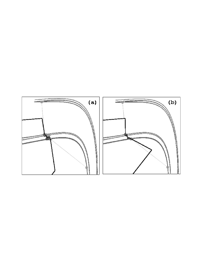
Figure 13: (a) Parameterizing a partition with reference points belonging to triangles bearing different symbols and whose mediators are located inside the shadow polygon yields a partition that cannot be distinguished from the original, yet has a much more compact description. (b) The number of reference points can be further reduced by keeping only those whose removal would change the encoding of one of the detected points.

Going back to the core ideas of the algorithm, we can achieve a much more compact description if we allow the border to be slightly displaced, but without modifying the encoding of any periodic point. Consider periodic points located in the Voronoï domain $V_{p}$ of a given reference point $p$. If the second nearest neighbors of all these points have the same symbol as $p$, $p$ can be safely removed without modifying the symbols that the partition assigns to any periodic point. To simplify the partition, one can therefore search for such reference points until further removals would change the encoding of some periodic points.

To achieve a compact parameterization, we have proceeded as follows. Given a periodic point $O_{i}^{j}$ located in region $\Delta_{s}(\Gamma)$, we define $n_{r}(O_{i}^{j})$ as being the number of reference points with symbol $s$ which are closer than the closest reference point with symbol $s^{\prime}\neq s$. Then, the redundancy of each reference point $p$ is estimated by $r(p)=\min_{O\in V_{p}}n_{r}(O)$.

We then remove the reference points with the highest $r(p)$ until the number of removed points is equal to the highest $r(p)$ for the remaining points, so as to ensure that for each periodic point there is still a nearest neighbor with the correct symbol. Indeed, a high value of $r(p)$ indicates that $p$ carries little information, as at least $r(p)$ reference points, including $p$, can be removed before the symbols associated to periodic points $O\in V_{p}$ are modified. This step is repeated until no reference point can be removed.

We have applied this procedure to the partition shown in Fig. 13a, and obtained a simplified partition (displayed in Fig. 13b) which is parameterized by only 8 reference points, yet has the same precision (of the order of 0.1% of the attractor width) as the original partition $\Gamma_{a}^{f}$ (Fig. 1b).

It can be seen on Fig. 13b that a compromise has to be found between compactness and robustness to noise. Indeed, with a small number of reference points, the partition line tends to wiggle and to pass close to a large number of periodic points, which increases the probability of encoding errors due to noise. A satisfying balance between these two requirements can be tuned for example by allowing the removal of a reference point $p$ only if $r(p)>r_{\text{min}}$, where $r_{\text{min}}$ is appropriately chosen. Our current selection algorithm can probably be much improved. However, the partitions of Fig. 13 show clearly that a high resolution can be achieved at a minimal cost. Furthermore, it should be recalled that in practical applications, such as chaos-based communication, the system trajectory is usually forced to stay at a finite distance of the partition border, which should allow one to simplify the description even more.

To conclude this section, we would like to show with a simple example that the method we have presented here has modest computational requirements when we limit ourselves to resolutions relevant to practical applications, and that it is well suited to perform a real-time encoding of a chaotic system.

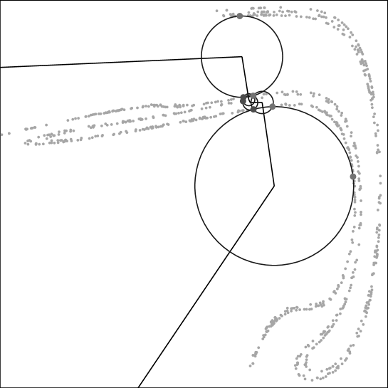
Figure 14: Partition obtained with a small set of periodic orbits (shown in grey), parameterized with only 7 points. The circumcenters delimiting the uncertain region are also displayed.

To this end, we computed a cover of the attractor of Fig. 1b with UPO of period up to $15$, and with a resolution of 3%, obtained with 75 periodic orbits. We applied to this set of UPO the standard algorithm described in [1]. The resulting partition was then simplified as described above to obtain the partition of Fig. 14 whose description utilizes only $7$ reference points. The computational costs of the different stages of the algorithm are given in Table 4 and can be seen to be very small. Yet, in spite of its much lower precision, the partition shown in Fig. 14b is characterized by exactly the same irreducible forbidden words as the high-resolution partition $\Gamma_{h}^{f}$ (see Sec. 2), at least up to length 19 included. Remarkably, we observed the same agreement for a similar partition based on 43 orbits of periods up to $12$ which displayed a much wider gap around the border.

This example clearly shows that experimental systems can be precisely characterized using the topological approach. It should be noted that for regimes that have a higher topological entropy, such as these found after the period-$3T$ crisis as in Ref. [2], a higher precision can be obtained using lower-period orbits. Also, the partition shown in Ref. [2] shows that even if most of the periodic orbits of period larger than 10 are very difficult to detect, this is in general not the case for those located just near the border line, as they are weakly unstable.

Table 4: Computational cost of the different stages of this algorithm for the partition of Fig. 14. CPU times are given for a Pentium 133 computer running under the Linux operating system.

Task	CPU time (seconds)
UPO detection	287.5
Computation of topological invariants	47.9
Template determination	0.9
Determination of topological names	2.0
Construction of the partition	5.4

9 Conclusion

In this work, we have carried out precise tests of the validity of the algorithm presented in [1]. A first indication that the resulting encodings faithfully describe the dynamics is that partitions determined from different initial configurations are equivalent: they encode a given trajectory in the same way, up to a shift of the symbolic sequences (Sec. 3). Furthermore, we have also directly verified that these partitions closely meet the criteria for being a generating partition by (i) observing that symbolic sequences of increasing length were associated to regions of decreasing diameters (Sec. 6), and (ii) by obtaining good estimates for the metric entropy from a long chaotic sequence (Sec. 7).

However, the most convincing evidence of the relevance of our method is provided by the perfect agreement between our results and those obtained by the classical method based on homoclinic tangencies. Indeed, we have found that important lines of homoclinic tangencies are entirely located inside the triangles enclosing the border of the partition (Sec. 5). This does not only mean that the partitions we obtain are very close to what is conjectured to be the correct solution, but also that our method naturally provides reliable error bounds, which are determined from the circumcircles of the triangles enclosing the partition border.

Even if the ultimate precision we can reach is probably lower than with homoclinic tangencies, the topological approach to constructing symbolic encodings has several distinctive advantages.

First, the problem of how to choose the tangency lines that will define a good partition is naturally solved. This was illustrated by the study of the Duffing attractor (Sec. 4.2). In this example, our algorithm naturally selects the lines of homoclinic tangencies that were found in Ref. [10] to yield the correct partition although some of them do not correspond to lines of primary homoclinic tangencies. That the solutions so obtained are the most natural ones is confirmed by the results of Sec. 3 where it was found that the different solutions were images or preimages of each other.

Second, the determination of the underlying template automatically indicates the correct number of symbols on which the dynamics is based. This is because this number is nothing but the number of branches of the template. This is also a key property since we have seen that for a given system, the number of symbols may depend on the parameter values as is the case, e.g., for the modulated laser system (compare the partitions shown in Figs. 1b and 5).

Last but not least, the topological approach should be extremely robust to noise. Indeed, it makes use of trajectories located in the whole phase space, and only gradually converges to the lines of homoclinic tangencies, where it is known that a dramatic noise amplification takes place [17]. The latter phenomenon is likely to adversely affect the determination of the directions of the invariant manifolds in the neighborhood of the tangencies from the time series, especially as the most expanding direction is orthogonal to the unstable manifold [17] there.

In contrast with this, the very fact that at homoclinic tangencies noise perturbs trajectories orthogonally to the unstable manifold implies that the locations of periodic points as estimated from close returns will be in first approximation displaced in a direction that is parallel to the border of the partition. The latter should thus be minimally affected, unless noise is so strong as to make the periodic point appear to be in different leaf of the attractor than the one it belongs to. Furthermore, it should be noted that the determination of topological invariants is relatively insensitive to noise level as the knot type of an orbit generally still can be exactly determined from an noisy, approximate trajectory shadowing this orbit.

All these properties clearly show that the topological approach should be a method of choice to construct generating partitions from experimental time series. As a matter of fact, we recall that a preliminary version of our algorithm has already been successfully applied to obtain with a very good accuracy a generating partition for a chaotic attractor of a modulated laser [2]. The relevance of template analysis to study the symbolic dynamics of experimental systems is further confirmed by the observation in Secs. 6 and 8 that a precision of only a few percent is sufficient to characterize very precisely the grammar of a chaotic regime.

We believe that our algorithm, and the way in which partitions are parameterized, could also prove useful in practical applications, and especially for transmitting information over chaotic signals, as proposed by Hayes, Grebogi and Ott [18, 19]. In this approach, the message to be transmitted is first encoded into a sequence of symbols that is compatible with the symbolic dynamics of the transmitting device. Then, tiny perturbations are applied to this device so that among all possible chaotic trajectories, it follows the one whose associated symbolic sequence is the given sequence. Indeed, we showed in Sec. 8 that once the partition has been determined, it is possible to simplify very much its description, so that encoding a signal merely amounts to finding among a few reference points which is closest to the point in phase space representing the current state of the system. This computation could easily be implemented in a digital signal processor, to achieve real-time encoding at the receiving side of the transmission line and recover thereby the digital message.

The fact that the images of a given partition can be easily and exactly computed (reference points are periodic) would also be beneficial at the sending side because it makes it easier to predict the next symbols that the device would emit if it was free-running, and thus to compute the tiny perturbation needed to synchronize the symbolic stream with the prescribed sequence. Finally, we note that our algorithm naturally selects a region where the encoding is to be considered uncertain, and which the transmitting device should not visit in order to avoid any ambiguity at the receiving side.

In conclusion, we believe that the present work shows that topological analysis, in the present form or in future extensions, is a promising tool to master the symbolic dynamics of experimental chaotic systems, especially given its robustness to noise and its ability to select the appropriate tangency lines and the correct number of symbols.

References

- [1] J. Plumecoq and M. Lefranc, “From template analysis to generating partitions I: description of the algorithm” (unpublished).
- [2] M. Lefranc, P. Glorieux, F. Papoff, F. Molesti, and E. Arimondo, “Combining topological analysis and symbolic dynamics to describe a strange attractor and its crises”, Phys. Rev. Lett. 73, 1364–1367 (1994).
- [3] G. B. Mindlin, X.-J. Hou, H. G. Solari, R. Gilmore, and N. B. Tufillaro, “Characterization of strange attractors by integers”, Phys. Rev. Lett. 64, 2350–2353 (1990).
- [4] G. B. Mindlin, H. G. Solari, M. A. Natiello, R. Gilmore, and X.-J. Hou, “Topological analysis of chaotic time series data from Belousov-Zhabotinski reaction”, J. Nonlinear Sci. 1, 147–173 (1991).
- [5] R. Gilmore, “Topological analysis of chaotic dynamical systems”, Rev. Mod. Phys. 70, 1455–1530 (1998).
- [6] N. B. Tufillaro, T. A. Abbott, and J. P. Reilly, An Experimental Approach to Nonlinear Dynamics and Chaos (Addison-Wesley, Reading, 1992).
- [7] H. G. Solari, M. A. Natiello, and G. B. Mindlin, Nonlinear Dynamics: a Two-Way Trip from Physics to Math (IOP Publishers, London, 1996).
- [8] J. S. Birman and R. F. Williams, “Knotted periodic orbits in dynamical systems I: Lorenz’s equations”, Topology 22, 47–82 (1983).
- [9] R. W. Ghrist, P. J. Holmes, and M. C. Sullivan, Knots and Links in Three-Dimensional Flows, Vol. 1654 of Lecture Notes in Mathematics (Springer, Berlin, 1997).
- [10] F. Giovannini and A. Politi, “Homoclinic tangencies, generating partitions and curvature of invariant manifolds”, J. Phys. A: Math. Gen. 24, 1837–1848 (1991).
- [11] P. Grassberger and H. Kantz, “Generating partitions for the dissipative Hénon map.”, Phys. Lett. A 113, 235–238 (1985).
- [12] P. Grassberger, H. Kantz, and U. Moenig, “On the symbolic dynamics of the Hénon map”, J. Phys. A 22, 5217–5230 (1989).
- [13] P. Cvitanovic, G. H. Gunaratne, and I. Procaccia, “Topological and metric properties of Hénon-type strange attractors.”, Phys. Rev. A 38, 1503–1520 (1988).
- [14] G. D’Alessandro, P. Grassberger, S. Isola, and A. Politi, “On the topology of the Hénon map”, J. Phys. A: Math. Gen. 23, 5285–5294 (1990).
- [15] R. Gilmore and J. W. L. McCallum, “Structure in the bifurcation diagram of the Duffing oscillator”, Phys. Rev. E 51, 935–956 (1995).
- [16] G. Boulant, M. Lefranc, S. Bielawski, and D. Derozier, “A non-horseshoe template in a chaotic laser model”, Int. J. Birfurcation Chaos Appl. Sci. Eng. 8, 965–975 (1998).
- [17] L. Jaeger and H. Kantz, “Homoclinic tangencies and non-normal Jacobians - effects of noise in nonhyperbolic chaotic systems”, Physica D 105, 79–96 (1997).
- [18] S. Hayes, C. Grebogi, and E. Ott, “Communicating with chaos”, Phys. Rev. Lett. 70, 3031–3034 (1993).
- [19] S. Hayes, C. Grebogi, E. Ott, and A. Mark, “Experimental control of chaos for communication”, Phys. Rev. Lett. 73, 1781–1784 (1994).
- [20] E. Bollt, Y.-C. Lai, and C. Grebogi, “Coding, channel capacity and noise resistance in communicating with chaos”, Phys. Rev. Lett. 79, 3787–3790 (1997).
- [21] J.-P. Eckmann and D. Ruelle, “Ergodic Theory of Chaos and Strange Attractors”, Rev. Mod. Phys. 57, 617–656 (1985).
- [22] P. Grassberger, “Finite sample corrections to entropy and dimension estimates”, Phys. Lett. A 128, 369–373 (1988).
- [23] R. Badii and A. Politi, Complexity : Hierarchical structures and scaling in physics, Vol. 6 of Cambridge Nonlinear Science Series (Cambridge University Press, Cambridge, 1997).