From template analysis
to generating partitions I:
Periodic orbits, knots and symbolic encodings

Abstract

We present a detailed algorithm to construct symbolic encodings for chaotic attractors of three-dimensional flows. It is based on a topological analysis of unstable periodic orbits embedded in the attractor and follows the approach proposed by Lefranc et al. [Phys. Rev. Lett. 73, 1364 (1994)]. For each orbit, the symbolic names that are consistent with its knot-theoretic invariants and with the topological structure of the attractor are first obtained using template analysis. This information, and the locations of the periodic orbits in the section plane, are then used to construct a generating partition by means of triangulations. We provide numerical evidence of the validity of this method by applying it successfully to sets of more than 1500 periodic orbits extracted from numerical simulations, and obtain partitions whose border is localized with a precision of 0.01%. A distinctive advantage of this approach is that the solution is progressively refined using higher-period orbits, which makes it robust to noise, and suitable for analyzing experimental time series. Furthermore, the resulting encodings are by construction consistent in the corresponding limits with those rigorously known for both one-dimensional and hyperbolic maps.

1 Introduction

Symbolic dynamics is a powerful approach to chaotic dynamics. It consists in representing trajectories in a chaotic attractor by sequences of symbols from a finite alphabet, in a way that preserves the essential properties of the dynamics [1, 2, 3, 4]. It is not only central to some of the most fundamental theorems of dynamical systems theory (see, e.g., [1, 2]), but can also be of utmost importance with a view to practical applications, such as for transmitting numeric streams over chaotic signals [5, 6].

However, we currently have a good understanding of how to construct symbolic encodings in two limiting cases only, namely for hyperbolic systems and non-invertible maps of an interval into itself [1, 2, 3, 4]. Unfortunately, most experimental low-dimensional systems fall outside these two categories, except when they are sufficiently dissipative so that their return maps can be modeled by one-dimensional maps.

To generalize one-dimensional symbolic dynamics to two-dimensional invertible maps and hence to flows, methods have been proposed that proceed by localizing homoclinic tangencies, i.e., points where the stable and unstable manifold of the attractor are tangent to each other [7]. Because this involves computing tangent maps and estimating their eigendirections, these methods require that the evolution equations are known, or at least that a model of the dynamics is available.

In this article, we present in detail a completely different approach. It is based on a topological analysis of chaotic data [8, 9, 10, 11, 12], and extracts information not only in the neighborhood of the singularities, but from the geometrical structure of the whole phase space. More precisely, the way in which stretching and folding act on the infinite number of unstable periodic orbits (UPO) embedded in any strange attractor is exactly reflected in the way these orbits are knotted and intertwined.

Stretching and folding are intimately related to symbolic dynamics. Because a systematic study of the knots and links realized by periodic orbits is made possible by template theory [13, 14] and template analysis [11, 12], precise information about the symbolic dynamics of the UPO can be extracted from their topological invariants. As we show in this work, this information, combined with the knowledge of the locations of the periodic points in the section plane, allows one to determine an excellent approximation to the border of a generating partition. This method does not involve the differentiable structure of return maps at all, and uses the concept of distance only to define neighborhoods, more precisely to determine which member of a set of reference points is nearest to a given point.

As this approach has already been applied to experimental time series from a modulated laser using a preliminary version of the algorithm described here [15], the primary goal of this article is to provide numerical evidence of the validity of the method. We thus apply it to more than 1500 UPO extracted from numerical simulations, and show that it is possible to obtain partitions which have a simple structure, yet are completely consistent with the topological organization of the UPO: the set of symbolic names assigned by the partition to the UPO corresponds to a set of orbits of the horseshoe template which have exactly the same topological invariants as the extracted ones. Direct evidence of the fact that partitions obtained in this way are generating will be presented in the second part of this work [16].

The article is organized as follows. In the remaining of this introduction, we recall the links between the geometric properties of chaos (stretching and folding) and symbolic dynamics. We then briefly review the approach based on homoclinic tangencies, and we finally illustrate the connection between symbolic dynamics and knot theory.

This connection can be precisely stated using template theory [13, 14] and template analysis [11, 12]. Since this approach to chaotic dynamics is not widely known, Sec. 2 is devoted to a review of its main concepts. We put emphasis on the relation between the symbolic name of an orbit and its topological invariants by giving examples of the analytical formulas linking them, and specify our fundamental assumptions.

In Sec. 3, we describe our algorithm in detail by progressively building a generating partition for a sample set of UPO extracted from numerical simulations of a modulated laser. We finally obtain a partition that is localized with a precision of the order of 0.01% of the attractor width. Last, we conclude by discussing possible extensions and applications of our method.

1.1 Stretching, folding, and symbolic dynamics

A striking feature of nonlinear dynamical systems is that they can display complex behavior even when obeying simple equations of motion. This seemingly paradoxical fact can only be understood by using a geometric description of the dynamical laws, in which they are represented as transformations of a phase space into itself. As is by now commonly known, there are simple such transformations that generate chaotic behavior by combining stretching and folding mechanisms (as in, e.g., the Rössler system).

In the last decades, several methods have been proposed to characterize a strange attractor, and thereby the underlying dynamics [17]. Not surprisingly, some of the most popular measures of chaos are deeply linked with the existence of the stretching and folding mechanisms. For example, Lyapunov exponents quantify the efficiency of stretching by estimating the rate of divergence of infinitely close trajectories. Spectra of fractal dimensions, and especially the correlation dimension as computed with the Grassberger-Procaccia algorithm, have been widely used to analyze the fractal structure that results from the repeated action of stretching and folding.

Symbolic dynamics is another approach to chaotic dynamics that is deeply rooted in the existence of the stretching and folding mechanisms. The connection between symbolic dynamics and the geometric properties of chaos is probably best illustrated by the paradigmatic Smale’s horseshoe map (Fig. 1), which is a key example to understand the link between the geometric features of chaos, symbolic dynamics and topological concepts.

If two points are not located on the same segment of the stable manifold (i.e., along an horizontal line), their forward iterates will eventually fall in different strips because of stretching. In the opposite case, so will do the backward iterates because of squeezing. Assigning distinct symbols to the two strips thus allows one to carry out a symbolic dynamical study of this map, each point of the invariant set being associated to a unique bi-infinite binary sequence. For a detailed presentation of the Smale’s horseshoe map in the context of topological analysis, see Refs.[18, 19, 8, 9, 10].

Figure 1: Representation of the action of the Smale’s horsehoe map. A unit square is first stretched along the unstable direction and squeezed along the stable direction, then folded over itself so that it intersects the original square in two disjoint strips.

In general, the symbolic encoding of a chaotic attractor is performed by dividing a Poincaré section into a few disjoint regions associated with distinct symbols (see Fig. 2). In the case of reversible equations of motion, each point of the attractor is then associated to the bi-infinite sequence made of the symbols corresponding to the regions visited by its backward and forward iterates.

More precisely, consider a partition $\Gamma$ of the section plane $P$ in $n$ disjoint regions $\Delta_{i}(\Gamma)$, $i=0,..,n-1$. Assume that for each point $x\in P$, $s_{\Gamma}(x)$ indicates the region which contains $x$: $s_{\Gamma}(x)=i$ if $x\in\Delta_{i}(\Gamma)$.

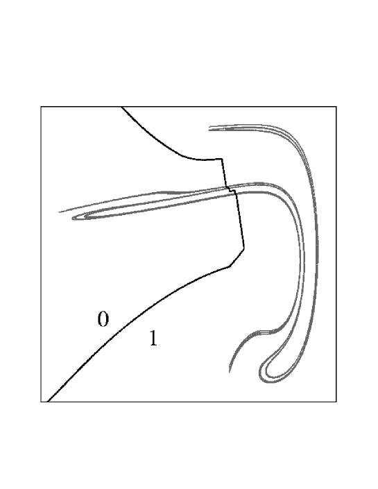
Figure 2: Symbolic encoding of a chaotic attractor using a partition of a section plane into two disjoint regions. This Poincar section has been obtained from the modulated laser equations (7) described in Sec. 3.1.

The point $x$ is then represented by a bi-infinite symbolic sequence

$$\Psi(x)=\{\ldots,\Psi_{-1}(x),\Psi_{0}(x),\Psi_{1}(x),\ldots\},\quad\Psi_{i}(x)=s_{\Gamma}(f^{i}(x)),$$

where $f$ is the Poincaré return map. Defining the shift operator $\sigma$ so that the sequence $\Psi^{\prime}(x)=\sigma\Psi(x)$ is made of the symbols $\Psi^{\prime}_{i}(x)=\Psi_{i+1}(x)$, it is readily seen that $\sigma$ represents the action of the return map in the space of symbolic sequences, as $\sigma\Psi(x)=\Psi(f(x))$ by definition.

Under certain conditions, such a coarse-grained measurement suffices to provide an accurate description of the dynamics: two different points, however close they may be, are associated to different symbol sequences; the partition is then said to be generating [2]. Of course, this is due to the amplifying action of stretching, which connects arbitrarily small length scales with large ones.

Symbolic dynamics can be given a rigorous foundation in the case of hyperbolic systems, such as the Smale’s horseshoe map shown in Fig. 1. Indeed, hyperbolicity allows one to define partitions (Markov partitions) that can be shown to be generating [2]. In this context, symbolic dynamics is of utmost importance to prove several fundamental theorems of dynamical system theory. For example, a symbolic dynamical analysis of the horseshoe dynamics easily shows that the invariant set contains aperiodic orbits, a dense infinity of unstable periodic orbits, and that there is at least one orbit which is dense in the invariant set [1, 2].

For non-hyperbolic systems, rigorous results are known only in the case of non-invertible maps of an interval into itself, such as the well-known logistic map. In this case, a generating partition is obtained by dividing the one-dimensional interval into regions where the map is monotonic: the border of the partition consists of the critical points of the map, where the derivative vanishes [1, 3, 4].

However, most strange attractors encountered in experimental systems or numerical simulations are non-hyperbolic: orbits are created and destroyed as a control parameter is varied, which is incompatible with the structural stability implied by hyperbolicity. Moreover, one-dimensional symbolic dynamics can only be used for extremely dissipative systems, and even then only in an approximate way. Whether symbolic dynamics can be put on a sound basis in the general case thus remains an open and fascinating problem.

A guiding fact is that the parameter space of a dynamical system such as, e.g., the Hénon map $(x,y)\rightarrow(a-x^{2}+by,x)$ contains generally both the hyperbolic and one-dimensional limits. For a sufficiently large value of the $a$ parameter, the Hénon map has an invariant hyperbolic repellor; it becomes equivalent to the one-dimensional map $x\rightarrow a-x^{2}$ when the $b$ parameter goes to zero. Therefore, a general procedure for constructing a symbolic encoding of a non-hyperbolic, weakly dissipative, attractor should have the one-dimensional and hyperbolic codings as limiting cases.

1.2 Symbolic encodings based on homoclinic tangencies

Accordingly, the method proposed by Grassberger and coworkers [7, 20] is a generalization of the one-dimensional theory. For a 1D map, the border of the partition naturally consists of the critical points of the map, whose existence is responsible for the non-invertibility of the map. In the case of invertible 2D maps, there are no critical points, but their natural counterparts are the homoclinic tangencies, where the stable and unstable manifolds of the attractor are tangent to each other. Their existence stems from the non-hyperbolicity of the map: in a sense, an invertible 2D map loses invertibility at homoclinic tangencies when iterated an infinite number of times. Furthermore, points of homoclinic tangency converge to backward and forward images of the critical points of the 1D map when dissipation is increased to infinity.

Grassberger and Kantz thus conjectured that a good symbolic encoding could be obtained by dividing the plane with a line connecting homoclinic tangencies [7, 20]. Several studies have given numerical evidence that the partitions so obtained were generating to a high level of accuracy [7, 20, 21, 22, 23, 24]. Another motivation for this rule is the fact that points located on opposite sides of a homoclinic tangency converge to each other both for positive and negative time. Thus, they can only be distinguished if they are associated to different symbols.

However, this approach has been rarely used, if ever, to characterize the symbolic dynamics of experimental chaotic time series (see however Ref. [25] for an application to time series generated from numerical simulations). Indeed, it heavily relies on the knowledge of the equations of motion and on the computation of the tangent map to determine the location of the homoclinic tangencies. While the direction of the invariant manifolds could in principle be estimated by fitting a model to the dynamics in the neighborhood of a point [25], the application of such a procedure to experimental time series seems hazardous. Indeed, it is a known fact that there is a dramatic noise amplification precisely at homoclinic tangencies [26]: since the stable manifold is tangent to the unstable manifold, it cannot drive perturbed trajectories back to the attractor. In this situation, extracting information from a tangent map constructed by estimating derivatives appears to be problematic.

Furthermore, it should be noted that this method is faced with the difficulty of choosing which homoclinic tangencies to connect, because all images and preimages of a homoclinic tangency are themselves homoclinic tangencies. To address this problem, Ref. [23] proposed to use only the so-called “primary” homoclinic tangencies, i.e., tangencies such that the sum of the curvatures of the stable and unstable manifolds is smaller than for all their images and preimages. Another approach to solving this problem was presented in Ref. [24], where the global organization of the lines of homoclinic tangencies in the phase space was studied.

This ambiguity is due to the fact that techniques based on homoclinic tangencies focus on the singularities induced by folding in the limit of infinite time. However, it is known from singularity theory (see, e.g., Ref. [27]) that singularities at a point organize the structure of an extended neighborhood of this point. Accordingly, there should be prints of the folding process in the whole phase space.

Indeed, there is another approach to the construction of symbolic encodings that focuses on the global organization of the strange attractor: it is based on a topological analysis of its unstable periodic orbits. That topological invariants of an unstable periodic orbit provide key information about the associated symbolic dynamics was, to our knowledge, first noted by Solari and Gilmore [28]. A method to construct a generating partition based on this idea was then outlined by Lefranc et al. [15] and applied to experimental time series from a modulated laser. Note that the fact that a generating partition assigns different names to different periodic orbits has also independently been used to construct symbolic encodings in Refs. [29, 30, 31].

1.3 From unstable periodic orbits and knot theory to symbolic dynamics

A strange attractor is not the only invariant set of a chaotic dynamical system, as it typically has embedded in it an infinite number of unstable periodic orbits (UPO). While these UPO, whose existence is due to ergodicity of chaotic dynamics, are known since the works of Poincaré, they have only been fully utilized to characterize and control chaos in the last decade (see, e.g., Refs. [32, 33, 34, 12, 31]). As we see in the following, they also prove to be invaluable for extracting symbolic dynamical information from experimental data.

As every trajectory in the attractor, unstable periodic orbits experience stretching and folding. But, as they exactly return to their initial condition in a short amount of time, they bear the mark of these mechanisms in a very distinct way: their associated closed curves in phase space are braided in a way that precisely reflects the action of stretching and folding (see Fig. 3). Because symbolic dynamics is also intimately related to stretching and folding, the way in which periodic orbits are intertwined must carry symbolic dynamical information.

Figure 3: Stretching and folding braid a periodic orbit in a definite way, as can be seen here with a period-4 orbit.

What makes this simple observation so fruitful is that this relation can be expressed in well-defined mathematical terms for strange attractors that can be embedded in a three-dimensional phase space. Indeed, characterizing the topological structure of closed curves in such a space is nothing but the central problem of knot theory (see e.g. [35]). Knot theory provides us with topological invariants that can be utilized to decide whether two closed curves can be continuously deformed into each other, i.e. have identical knot types or not, and thus to classify periodic orbits according to their geometrical structure.

The relevance of knot theory in the context of dynamical system theory stems from one of its fundamental theorems. Indeed, the uniqueness theorem states that one and only one trajectory passes through a non singular point of phase space (because of determinism). In particular, this implies that a periodic orbit cannot intersect itself, nor another orbit, and thus that the knots and links they form have a well-defined type. Moreover, changing a control parameter will usually change the shape of a periodic orbit but, for the same reason, will not induce intersections. Consequently, the knot type of a periodic orbit remains unchanged on the whole domain of existence of the orbit, and can be viewed as a genuine fingerprint.

It is thus obvious that topological invariants from knot theory provide us with a robust way to characterize how stretching and folding intertwine unstable periodic orbits. As an example, the simplest topological invariant, the linking number, indicates how many times one orbit winds around another. What makes these invariants relevant for experimental studies is their robustness. If two periodic orbits are sufficiently separated, knot invariants can be reliably determined even when only approximate trajectories, possibly contaminated by noise, are available (as typically extracted from a time series). Indeed, the possible perturbations then merely amount to small deformations of the orbit and do not change the invariants.

It should be noted that because the topological approach relies on knot theory, it can only be applied to flows and hence to orientation-preserving two-dimensional return maps. Thus, orientation-reversing 2D return maps, such as the Hénon map at the standard parameters $(a=1.4,b=0.3)$, fall outside its scope. However, this will allow us to show that phenomena that have been observed in such maps [36, 37] violate the more restrictive constraints obeyed by orientation-preserving return maps.

The link between topological invariants and symbolic dynamics is provided by the tools of template theory. Since the main concepts of the latter are not widely known, we review them in the next section, before presenting the details of our algorithm in Sec. 3.

2 Periodic orbits, knots and templates

2.1 Template theory of hyperbolic systems: the Birman–Williams theorem

As is the case for many features of chaotic behavior, most of the rigorous results about the topological structure of unstable periodic orbits are known in the context of hyperbolic dynamical systems. They compose what may be called template theory [14]. The keystone of the latter is the Birman-Williams theorem [13, 38], which shows that the topological organization of the unstable periodic orbits of an hyperbolic flow can be studied in a systematic way.

Given a hyperbolic chaotic three-dimensional flow $\Phi_{t}$ with an invariant set $\Lambda$, let us define an equivalence relation between points of $\Lambda$ in the following way:

$$\forall x,y\in\Lambda,\quad x\sim y\Leftrightarrow\lim_{t\rightarrow\infty}||\Phi_{t}(x)-\Phi_{t}(y)||=0,$$ (1)

which relates points having the same asymptotic future. Identifying points in the same equivalence class thus amounts to collapsing the invariant set along its stable manifold. The Birman-Williams theorem [13, 38] consists of two main statements:

1. In the set of equivalence classes of relation (1), the hyperbolic flow $\Phi_{t}$ induces a semi-flow $\bar{\Phi}_{t}$ on a branched manifold $\mathcal{K}$. The pair $(\bar{\Phi}_{t},\mathcal{K})$ is called a template, or knot-holder, for a reason that is made obvious by the second statement.

2. Unstable periodic orbits of $\Phi_{t}$ in $\Lambda$ are in one-to-one correspondence with unstable periodic orbits of $\bar{\Phi}_{t}$ in $\mathcal{K}$. Moreover, each unstable periodic orbit of $(\Phi_{t},\Lambda)$ is isotopic to the corresponding orbit of $(\bar{\Phi}_{t},\mathcal{K})$, the same property holding for any link made of a finite number of UPO. Thus, periodic orbits in the invariant set can be continuously deformed without any crossing so as to be laid on the branched manifold.

The second statement implies that any topological invariant defined in the framework of knot theory will take identical values on a set of UPO of the flow and on the corresponding set of periodic orbits of the template.

The proof of the Birman-Williams theorem relies on a key property: two points belonging to the same periodic orbit, or to different periodic orbits, have by definition different asymptotic futures; if initially separated, they will remain at a finite distance forever. Thus, a periodic orbit cannot intersect its own stable manifold, nor the stable manifold of another orbit. As a result, collapsing the invariant set along its stable manifold does not induce crossings between periodic orbits, hence does not modify their topological organization.

This simple observation is central to template theory and template analysis because it clearly shows that their concepts are insensitive to the degree of dissipation, which becomes irrelevant after reduction of the stable manifold. In a given topological class, any flow has the same global topological organization as an infinitely dissipative flow. This is precisely what will allow us to use template analysis as a bridge between one-dimensional and two-dimensional symbolic dynamics.

As an example, the Smale’s horseshoe template, i.e. the branched manifold corresponding to a flow whose return map is the Smale’s horseshoe map, is shown in Fig. 4. The number of branches, the torsions and linking numbers of its branches define the structure of such a manifold, as well as the order in which branches are stacked when they rejoin. The Smale’s horseshoe template presented in this form is an example of a fully expansive template: the branches are stretched to the full width of the template. This stretching, and the folding of branches over each other describe geometrically the basic mechanisms of chaotic dynamics. As will be recalled in Sec. 2.3, the topological structure of a template can be concisely described by a small set of integers which suffice to determine topological invariants of a closed curve on the template, given its itinerary on the branched manifold (i.e., the order in which it visits the different branches).

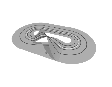
Figure 4: The Smale’s horseshoe template, with a period-1 and a period-4 orbits. In this configuration, these orbit have exactly the same invariants they would have in a hyperbolic flow whose topological structure is described by this template. Because the branches correspond to the disjoint strips shown in Fig. 1, a symbolic description of the closed curves of the template can be given.

For a more detailed exposition of the template theory of hyperbolic sets, we refer the reader to Refs. [13, 38, 39, 18, 40, 19, 41], and to a recent book by Ghrist, Holmes and Sullivan [14] for a comprehensive review.

2.2 Template analysis of experimental systems

The central problem of template theory is: given a hyperbolic template, what can we say about the properties of knots living on this template?

When we study an experimental system, however, the underlying template is not a priori known, but unstable periodic orbits can be extracted from time series, and their topological invariants and knot types determined in a reconstructed phase space. Note that, while a strange attractor is generally not hyperbolic, tools from template theory are still relevant because the existing orbits should have the same organization and the same invariants as in the hyperbolic limit, provided they can be brought to this limit by a change in control parameters.

In this context, the natural question then is: given a finite set of knots contained in the attractor, can we construct a template which holds all of them, and thus describes the global topological organization of the strange attractor?

This program was pioneered by Mindlin et al. [11], who proposed to use the concepts of template theory to characterize non-hyperbolic strange attractors by a small set of integers. They demonstrated and thoroughly discussed the relevance of this approach by showing in a beautiful work that all the topological invariants of periodic orbits detected in time series from the Belousov-Zhabotinskii chemical reaction allowed them to be globally laid on a Smale’s horseshoe template [12].

In the last decade, further evidence that the topological organization of experimental chaotic systems could be described by templates has been given in a variety of systems: a NMR oscillator [42], CO₂ lasers with a saturable absorber [43, 44], or with modulated losses [45, 15], a glow discharge [46], a copper electro-dissolution reaction  [47], a vibrating string [48], an electronic circuit [49], a fiber laser [50], or a YAG laser [51]. Similar conclusions have also been obtained in numerical simulations of the Duffing [52, 53], Lorenz [54], and Rössler equations [55], and for systems modeling a bouncing ball [56], pulsating stars [57], and lasers [58, 59].

All these studies follow more or less the same procedure [8]. First, segments of time series shadowing unstable periodic orbits are extracted from the experimental data, and are embedded in a reconstructed phase space, where the topological invariants of the associated closed curves are computed. Then the simplest template on which the experimental orbits can be projected is determined from the measured invariants. This is made possible by the fact that the relevant information is carried by low-period orbits. Indeed, the characteristic numbers of a template are completely determined by the invariants of its spectrum of period-1 and period-2 orbits [8].

The validity of a candidate template (determined from the lowest-period orbits) can then be checked by verifying that the invariants of the higher-period orbits allow them to be also laid on the template. This is because the template characteristic numbers are over-determined by the topological invariants of the unstable periodic orbits. In the case of the Smale’s horseshoe template, for example, four integers suffice to compute the invariants of an infinite number of periodic orbits. As we will show in the following, the seemingly redundant information carried by the topological invariants of a large set of UPO can be used to extract information about the symbolic dynamics of the attractor.

For further information, detailed introductions to template analysis can be found in in a comprehensive review article by Gilmore [8] and in books by Tufillaro, Abbott, and Reilly [9], and by Solari, Natiello, and Mindlin [10].

2.3 Extracting symbolic dynamical information from knot invariants

Our approach to the construction of symbolic encodings relies heavily on the mathematical link between the topological invariants of unstable periodic orbits and symbolic dynamics. To illustrate this link more precisely, we now review briefly some of the basic tools of template analysis.

As an example, we first consider the Smale’s horseshoe period-$4$ orbit that is created in the initial period-doubling cascade. We show how its simplest invariant, namely its self-linking number, is easily computed from its symbolic name, which is “0111” if we use the coding shown in Fig. 4.

The branch line of a fully expansive template (the line where the different branches are squeezed over each other) is a one-dimensional analogue of a global Poincaré section: each period-$n$ orbit intersects the branch line in exactly $n$ points. Because template orbits cannot intersect on the two-dimensional (branched) manifold, the layout of a periodic orbit on a template is completely determined by the order in which its intersections with the branch line are visited.

Computing this order is a classic exercise in symbolic dynamics of maps of an interval into itself [1, 3] (see Refs. [8, 9, 18] in the context of template analysis), since the return map of the branch line is one-dimensional. In the case of the Smale’s horseshoe template, this return map has the same structure as the standard logistic map, with the region of positive (resp. negative) slope corresponding to the branch with a torsion of zero (resp. one) half-turns. In our example, it is easily found that the periodic points of the period-$4$ orbit are found on the branch line in the order: “0111”, “1101”, “1110”, “1011”.

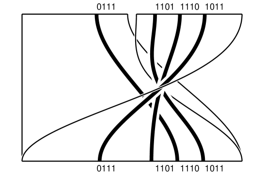
Figure 5: Geometry of the period-$4$ orbit “0111” on the template. Only the nontrivial part (i.e., the branched part) of the manifold is shown, as the top line can be identified with the bottom line (the branch line). The layout of the periodic points on the branch line is completely fixed by the fact that branches “0” and “1” are orientation-preserving and orientation-reversing, respectively. Given the geometrical structure of the branches, this layout determines in turn the braid associated with the orbit, and hence all its topological invariants.

As can be seen in Fig. 5, it then suffices to connect periodic points to their images by following the semi-flow on the branched manifold to obtain the braid associated with the orbit. In this case, it is straightforward to verify that the self-linking number of the “0111” orbit of the Smale’s horseshoe template is 5.

This simple example illustrates concisely the key idea that the symbolic dynamics of an unstable periodic orbit completely determines its knot invariants and that conversely, the latter carry important information about the former. We now want to stress that this property can be expressed by simple algebraic relations.

Following Mindlin et al. [11, 12], the structure of a $n$-branch template can be algebraically described by a $n\times n$ matrix, the template matrix, and a $1\times n$ matrix, the layering matrix. The template and layering matrices are related to invariants of low-period orbits in the following way.

Because the semi-flow on the branch manifold is expanding, each branch carries one and only one period-$1$ orbit. The template matrix $t$ is obtained from the organization of these period-$1$ orbits as follows. The diagonal elements $t_{ii}$ indicate the local torsion of the orbit on branch $i$, i.e. the rotation of its stable and unstable manifolds in units of $\pi$. Off-diagonal elements $t_{ij}=t_{ji}$ are equal to twice the linking number of the orbits located on branches $i$ and $j$. In the case of the Smale’s horseshoe with zero global torsion shown in Fig. 4, with branches labeled “0” and “1”, the template matrix reads:

$$t^{HS}=\left(\begin{array}[c]{cc}0&0\\ 0&1\end{array}\right)$$ (2)

where $t_{11}=1$ describes the folding of the “1” branch.

To complete the description of the template structure, one has to specify in which order the different branches are superimposed when they are glued together. Mindlin et al. define the $1\times n$ layering matrix $l$, which verifies $l_{i}<l_{j}$ iff branch $j$ is located above branch $i$ on the branch line. Since the twisted branch of the horseshoe template is folded over the untwisted one, its layering matrix is given by:

$${l}^{HS}=\left(\,0\,1\,\right)$$ (3)

We use a slightly different convention and introduce a $n\times n$ symmetric matrix $l^{\prime}$ such that for $i<j$, $l^{\prime}_{ij}=1$ if branch $j$ is located above branch $i$ and $l^{\prime}_{ij}=-1$ otherwise (i.e., $l^{\prime}_{ij}=-1$ indicates that the order of two branches differs from that of a standard layering graph as defined in Ref. [60]). For the horseshoe template, we thus have:

$${l^{\prime}}^{HS}=\left(\begin{array}[c]{cc}0&1\\ 1&0\end{array}\right)$$ (4)

A key property of template analysis is that simple analytic formulas can be written to express some of the topological invariants of the UPO as a function of the elements of the template and layering matrices [61], using techniques similar to these described in appendix E of Ref. [9]. These invariants are the (self-) linking numbers, relative rotation rates [28], and torsions of the periodic orbits. To predict more sophisticated invariants, such as knot polynomials, a description of the template as a framed braid (see, e.g., Ref. [60]) would be required.

For example, the self-linking number of the “0111” orbit is given for a general template by:

$$slk(0111)=3t_{01}+3t_{11}+(3-\pi(t_{11}))\times l^{\prime}_{01}$$ (5)

where $\pi(t)=1(0)$ if $t$ is odd (even). The reader may verify that the value of 5 that can be obtained from Fig. 5 is recovered by inserting in Eq. (5) the horseshoe template matrices given in Eqs. (2) and (4). Similar expressions can easily be obtained for invariants of orbits of arbitrarily high period. For example, we have:

$$lk(01^{3}0101^{2},\left(01^{2}\right)^{3}01^{4}01^{3}) = \frac{15}{2}t_{00}+39t_{11}+\frac{69}{2}t_{01}$$

$$+\left(30-\frac{19}{2}\pi(t_{11})-\frac{1}{2}\pi(t_{00}+t_{11})\right)\times l^{\prime}_{01}$$

where $lk(\alpha,\beta)$ denotes the linking number of orbits $\alpha$ and $\beta$.

A crucial property of these expressions is that, except for the presence of the terms involving the $\pi$ function, they are linear in the elements of the template matrices $t$ and $l^{\prime}$. This is what allows one to design a powerful algorithm to determine these elements from the topological invariants of a few orbits of low period: one considers all the possible symbolic names for these low-period orbits, and all the possible branch parities, and selects those that lead to a consistent, over-determined, set of linear equations. The solution to such a set of equations is a candidate template, whose validity has then to be checked with higher-period orbits. The general procedure will be described elsewhere [61], but some examples may be found in Refs. [50, 58].

When the geometry of the branched manifold of the template has been determined in this way, we then find all sets of symbolic names such that template orbits with these names have exactly the same invariants as the experimental periodic orbits. This indicates the different possible projections of the set of UPO on the branched manifold that preserve its topological organization.

In fact, there are only a few possible such projections for a given experimental orbit. For example, in the case of the Smale’s horseshoe template, there is one and only one period-$7$ orbit of even torsion with a self-linking number of 16: this is the “0101011” orbit. In this case, the symbolic name of this orbit can be unambiguously extracted from its topological structure. In some other cases, there may be several possible symbolic names. For example, the horseshoe orbits “001101” and “001011” correspond to isotopic knots and thus cannot be distinguished using the self-linking number or self-relative rotation rates. However, they often can be identified using other orbits which link them differently (if these orbits are found in the attractor): in the previous example, there are four period-$8$ horseshoe orbits whose linking numbers with the two period-$6$ orbits are different (e.g., $lk(00101011,001101)=15$ but $lk(00101011,001011)=14$.)

Table 1: Basic topological properties of the periodic orbits with period up to 9 extracted from numerical simulations of a modulated laser model (see Sec. 3.1), and that will be used as an example in Sec. 3. The listed invariants are: period, self-linking number, torsion. The symbolic names of horseshoe orbits with the same invariants are also displayed. Note that except for orbits 18 and 19, there is a single possible symbolic name. The two possible symbolic names for orbits 18 and 19 are related through a time-reversal symmetry of the Smale’s horseshoe template.

Orbit	Invariants	Names	Orbit	Invariants	Names
1a	1,0,1	“1”	8b	8,21,5	“01011011”
2a	2,1,1	“01”	8c	8,25,7	“01111111”
4a	4,5,3	“0111”	8d	8,25,6	“01011111”
5a	5,8,3	“01011”	8e	8,23,5	“01010111”
5b	5,8,4	“01111”	9a	9,28,7	“011011111”
6a	6,13,5	“011111”	9b	9,28,6	“010110111”, “010111011”
6b	6,13,4	“010111”	9c	9,28,6	“010110111”, “010111011”
7a	7,16,5	“0110111”	9d	9,28,5	“010101011”
7b	7,16,4	“0101011”	9e	9,30,7	“011101111”
7c	7,18,6	“0111111”	9f	9,32,8	“011111111”
7d	7,18,5	“0101111”	9g	9,30,6	“010101111”
8a	8,21,6	“01101111”	9h	9,32,7	“010111111”

This important fact is illustrated by Table 1 which shows an example where the symbolic names of all orbits up to period 9 extracted from an attractor, except two of them, can be obtained using only the simplest topological invariants. This implies that there are only two sets of horseshoe orbits which reproduce the measured invariants. These sets differ by the names given to orbits 9b and 9c.

Although it should be noted that it is more common for higher-order orbits to have several possible symbolic names, it appears very clearly from Table 1 that topological invariants carry a large amount of information on the symbolic dynamics of a chaotic system. As we now explain in Sec. 2.4, this is the property which the following of the article will rely on.

2.4 Topological encoding as a bridge between the one-dimensional and the hyperbolic encodings

As mentioned in Sec. 1.3, the topological structure of a given unstable periodic orbit is not modified by a change in a control parameter. If we assume that there is a parameter that allows us to freely tune dissipation, modifying this parameter will induce isotopic deformations of the unstable periodic orbits, thus preserving their topological structure (except for orbits that are annihilated or created in saddle-node bifurcations).

Returning to the example of Table 1, let us appropriately vary this control parameter so as to achieve infinite dissipation. In this limit, the dynamics should be modeled by a one-dimensional return map similar to the logistic map $x_{n+1}=a-x_{n}^{2}$. Because of the deep link between template theory of the Smale horseshoe and the symbolic dynamics of the logistic map, it is then obvious that the symbolic name given by one-dimensional symbolic dynamics theory will coincide with the one singled out by topological analysis and indicated in Table 1.

Let us now assume that by varying another parameter, we bring the system to a region of parameter space where it has an hyperbolic invariant set. Because template theory is mathematically rigorous in this case, the topological symbolic names in Table 1 must also be consistent with the ones obtained from a canonical Markov partition.

We will therefore make the fundamental hypothesis that any relevant symbolic encoding should assign to a given periodic orbit a name that is compatible with its topological structure, i.e. such that the orbit with the same name on the associated template has identical topological invariants. This is a strong assumption, as it implies that an orbit with a single topological name must be assigned the same name on its whole domain of existence (provided the global topological structure described by the template is not modified). However, this appears to be the only way to connect the two limiting cases in a continuous way.

Because this assumption is central to the method we describe below, it is important to note that it might seem to be contradicted by some observations reported in the literature. In particular, Hansen has described the following striking phenomenon [36]: by following a certain closed loop in the parameter space of the Hénon map starting and ending at parameters $(a=2,b=0)$ (where the one-dimensional canonical coding is available), the unstable periodic orbit with initial symbolic name “011111” is transformed into the orbit with symbolic name “000111”. This observation seems to indicate that there cannot be a global symbolic name in the whole parameter space. Similarly, Giovannini and Politi have pointed out that at some parameter values, the symbolic encodings of some periodic orbits can experience sudden changes due to the annihilation of primary homoclinic tangencies [37].

Although the Hénon map is generally considered to capture the essential features of low-dimensional chaotic dynamics, we believe that it would be incorrect to conclude from these studies that such discontinuities occur in all two-dimensional maps involving the creation of a horseshoe. More precisely, we highly suspect that the situation is dramatically different for orientation-preserving maps (i.e., maps that can be viewed as return maps of a three-dimensional flows), as the simple following argument shows.

In any suspension of a horseshoe-type map with zero global torsion, the self-linking number of the “011111” orbit is 13. There is only one other period-$6$ horseshoe orbits corresponding to this value: the “010111” orbit which is the saddle-node partner of the “011111” orbit. Since the latter can be distinguished from the former in that it has odd torsion (i.e., negative Floquet multipliers), there is absolutely no way in which the unstable “011111” orbit could be turned into another orbit by following a closed path in parameter space, provided this path stays on the orientation-preserving side of parameter-space. Under this condition, indeed, a suspension of the Hénon map that deforms continuously as the parameter is varied can easily be constructed.

Similarly, Giovannini and Politi have reported that at some parameters of the Hénon map (also in the orientation-reversing case), the partition line experiences a discontinuity in such a way that the substring “…11000…” has to be replaced by the substring “..01001…” in all the symbolic names of the periodic orbits [37]. Defining a $C_{n}$ orbit as an orbit whose symbolic name contains the substring “$0^{n-1}$”, but not “$0^{n}$”, this recoding would turn some $C_{4}$ orbits into $C_{3}$ orbits. Although one can find some examples of $C_{3}$ and $C_{4}$ orbits that have the same braid type, the two classes of orbits are easily distinguished through their linking numbers with other orbits [15, 28]. Thus, we have here another phenomenon where the change in the symbolic name is accompanied by a change in the topological invariants associated with this name.

Of course, our argument does not prove that the Hansen phenomenon cannot occur for higher-order orbits with a larger number of isotopic orbits (if they cannot be distinguished through their linking numbers with a third orbit). However, this clearly shows that there are effects which occur in orientation-reversing maps which would violate the uniqueness theorem in suspensions of orientation-preserving maps (because these effects connect symbolic names corresponding to different topological invariants). This somehow questions the relevance of the Hénon map at the classical parameters (where the Jacobian is negative) as a prototype of return maps in three-dimensional flows.

There is thus, to our knowledge, currently no clear counter-example to our hypothesis that well-defined symbolic encodings can be obtained for orientation-preserving maps. Therefore, we now proceed and describe how to construct generating partitions that are compatible with the topological invariants of the UPO. We will see that, while the algebraic tools of template analysis do not always select a single name for every orbit, a non-ambiguous encoding and a complete identification of the symbolic names are eventually obtained if we additionally require the symbolic encoding to be continuous, so that points which are close in a section plane are encoded by sequences that are close in sequence space.

3 Description of the algorithm

3.1 Detection of the unstable periodic orbits

As we have seen in Sec. 2, template analysis yields for each detected periodic orbits a list of possible symbolic names. The next step is to use this information and the locations of these periodic orbits in the section plane to construct a partition, which may then be used to encode chaotic trajectories as well.

To illustrate the procedure that we detail below, we will study a chaotic attractor observed in numerical simulations of a modulated class-B laser, described by the following equations [62, 63]:

$$\dot{I} = I[AD-1-m\sin\omega t]$$ (7a)

$$\dot{D} = \gamma\left[1-D(1+I)\right]$$ (7b)

where the variables $I$ and $D$ represent the output intensity and the population inversion. In our numerical simulations, the following parameters were used: $A=1.1$ (pump rate), $m=0.0334$ (modulation amplitude), $T=2\pi/\omega=300$ (modulation period), and $\gamma=2.5\times 10^{5}/1.2\times 10^{8}=2.083\times 10^{-3}$ (ratio of the population inversion relaxation rate to the cavity damping rate). Fig. 2 shows the Poincaré section in $(\log I,D)$ coordinates corresponding to $t=0\bmod T$ (as for all the Poincaré sections shown in this paper). The topological structure of this attractor is described by the Smale’s Horseshoe template shown in Fig. 4.

The algorithm we describe in this section will allow us to determine unambiguously the symbolic names of a set of unstable periodic embedded in the strange attractor. If we want to utilize this information to perform symbolic encodings of arbitrary trajectories, we must detect a set of orbits that provides a good cover of the attractor, i.e., which is such that all trajectories on the attractor are locally shadowed with a good precision by an UPO.

Our detection code was specially designed to achieve this goal. Basically, it divides the Poincaré section in cells of size $\epsilon$ and follows a long chaotic trajectory, searching for close returns. When one is found, we check whether all the cells visited by points in the corresponding time series segment contain periodic points of period lower than or equal to the recurrence time. If this is not the case, a Newton-Raphson iteration is started from this initial condition. When the latter succeeds, the quality of the cover has been improved. The search terminates when each cell contains at least one periodic point and when no significant improvement has been obtained over a certain interval of time (the detection of a periodic point of lower period than those already contained in the cell is considered as an improvement). In this way, the computational effort is concentrated on obtaining the most uniform cover with orbits of lowest periods, rather that finding the highest possible number of orbits.

This preliminary investigation revealed an interesting property: some parts of the strange attractor are extremely difficult to shadow with orbits of low period, especially when there are a lot of forbidden sequences in the symbolic dynamics. It turns out that these regions will be found later to be close to the partition border and to lines of homoclinic tangencies. If we view periodic and chaotic trajectories as the analogues of rational and irrational numbers, respectively, this observation could be rephrased as: near principal lines of homoclinic tangencies, chaotic trajectories are more “irrational” than elsewhere in the attractor. While this may seem to be a fundamental obstacle to our approach, it should be noted that because the dynamics is weakly unstable in these regions, it is easy to detect the high-period orbits which are located in them, and that topological invariants of high-period orbits can be computed robustly. This explains why, in spite of the above-mentioned effect, we will be able to localize partition borders to within 0.01% of the attractor width in Sec. 3.6. Furthermore, we will show in the second part of this work [16] that because of non-hyperbolicity, obtaining a high-resolution shadowing in these regions is in fact not at all crucial for characterizing accurately the symbolic dynamics.

Following the procedure described above with $\epsilon=0.001$ and with a maximal period of $32$, we obtained a set of 1594 periodic orbits providing a uniform cover of the attractor. This set of orbits will be used throughout this section to illustrate the different stages of our algorithm. The possible symbolic names of the lowest-period orbits as determined from template analysis have been given in Table 1.

3.2 Notations

The detected set of orbits will be noted $\mathcal{O}$, and consists of $m$ UPO $O_{i}$. Each periodic orbit $O_{i}$ has $p_{i}$ intersections $O_{i}^{j}$, $j=1,\ldots,p_{i}$, with the section plane ($p_{i}$ is the topological period of the orbit). These intersections are periodic points of the first return map $f$, and their set will be noted $\mathcal{P}$.

As we have seen in Sec. 2, knot theory and template analysis provide us for each orbit $O_{i}$ with one or several possible names. These “topological names”, which will be noted $\mathcal{N}_{k}(O_{i})$, are the names of the template orbits which have the same topological invariants. For definiteness, and since all cyclic permutations of a topological name represent the same orbit, we always write the topological name using the lowest permutation in the lexicographic order, enclosed inside brackets. For example, if the period-$2$ orbit $O_{2}$ can be named “01” or “10”, then $\mathcal{N}(O_{2})=\langle 01\rangle$.

Symbolic names are also used to label periodic points. In this case, cyclic permutations of a given string of symbols are not equivalent, since they correspond to different periodic points. In this context, we use overlined strings. For example, the intersection of the orbit $O_{2}$ with the section plane consists of two periodic points: $\overline{01}$ and $\overline{10}$.

A partition $\Gamma$ of the section plane into $n$ disjoint regions $\Delta_{i}(\Gamma)$ assigns to each UPO a symbolic name $N_{\Gamma}(O_{i})$. Because two partitions that associate a given periodic point with different cyclic permutations of the same name are to be considered different, we define $N_{\Gamma}(O_{i})$ as being the symbolic name of its first periodic point: $N_{\Gamma}(O_{i})$=$N_{\Gamma}(O_{i}^{1})$. The latter is made of the symbols associated with the regions containing by $O_{i}^{1}$, $O_{i}^{2}$,…,$O_{i}^{p}$.

3.3 Parameterization of partitions by periodic orbits

Let us first consider the period-$1$ and period-$2$ orbits $O_{1}$ and $O_{2}$ whose symbolic names can be unambiguously determined as being $\mathcal{N}(O_{1})=\langle 1\rangle$ and $\mathcal{N}(O_{2})=\langle 01\rangle$. The latter consists of two periodic points whose symbolic names are the cyclic permutations of $\mathcal{N}(O_{2})$, namely $\overline{01}$ and $\overline{10}$.

There are thus two possibilities for assigning a symbolic sequence to the two points $O_{2}^{1}$ and $O_{2}^{2}$ of the $O_{2}$ orbit. Either $\{N_{\Gamma}(O_{2}^{1}),N_{\Gamma}(O_{2}^{2})\}=\{\overline{01},\overline{10}\}$ or the opposite choice is made. As we will see in the second part of this work [16], these two possibilities lead to different, but dynamically equivalent, solutions. For definiteness, we restrict ourselves to the first configuration in this section.

In the following, we call reference points the periodic points whose symbolic sequence is assumed to be unambiguously known. We now explain how the three reference points $\{O_{1}^{1},O_{2}^{1},O_{2}^{2}\}$, associated with sequences $\{\overline{1},\overline{01},\overline{10}\}$, may be used to define a rough partition, which will be later refined by considering higher-order periodic orbits.

If we examine generating partitions such as these shown in Fig. 2 and in Refs. [7, 20, 22, 23], we note that the regions of the section plane corresponding to different symbols are separated by a line with a simple structure, whose length is of the order of the diameter of the attractor. Consequently, there is a high probability, as higher as the points are closer, that a point and one of its close neighbors correspond to the same symbol, except if they are located in a small region around the border.

If a point is in a close neighborhood of one of the three reference points, it is natural to encode this point with the same symbol as this reference point. For points which are at comparable distances from two or more reference points, the correct symbol is uncertain. However, without using the information that will be provided by the higher-order periodic orbits, the simplest procedure that is consistent with the previous remark is to associate these points with the symbol of the closest reference point. We thus have a simple rule to encode a chaotic trajectory: at each intersection with the section plane, the closest reference point is determined and the associated symbol is inserted in the symbolic sequence.

The corresponding partition of the section plane obtained using the three initial reference points is shown in Fig. 6. In this simple case, the border line of the partition is easily constructed, since one has merely to separate points whose nearest reference point has leading symbol “0” from those whose nearest reference point has leading symbol “1”. Thus, the partition border follows the mediators of the segments joining points with different symbols (i.e., the segments from $\overline{01}$ to $\overline{1}$ and from $\overline{01}$ to $\overline{10}$). It is a known geometrical property that these two mediators intersect at the circumcenter of the triangle made of the three initial reference points.

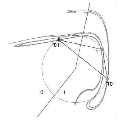
Figure 6: The initial partition based on periodic points $\overline{1}$,$\overline{10}$, and $\overline{01}$. For points that are at the left (resp. right) of the border, the closest reference point is the $\overline{01}$ periodic point (resp. one of the $\overline{1}$ and $\overline{10}$ periodic points). The circumcenter of the triangle made of the three points is also shown.

A nice property of the above rule is that it can be efficiently implemented for an arbitrary number of reference points, using well-known geometrical tools: Delaunay triangulations and Voronoï diagrams [64, 65, 66].

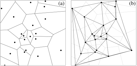
Figure 7: (a) Voronoï diagram of a set of points. (b) the corresponding Delaunay triangulation. The circumcenter of one of the triangles is shown.

Given a reference point $O_{i}^{j}$, the set of points in the section plane that are closer to $O_{i}^{j}$ than to any other reference point is nothing but the Voronoï domain of $O_{i}^{j}$ with respect to the set of reference points. The Voronoï diagram is a graph that consists of the borders of the Voronoï domains (Fig. 7a). The dual graph of the Voronoï diagram is called the Delaunay triangulation (Fig. 7b). Among the possible triangulations of a set of points, the Delaunay triangulation is the only one such that the circumcircle of a triangle linking three sites never contains another site [64, 65, 66]. This property can be used to implement efficient algorithms for building Delaunay triangulations, from which the associated Voronoï diagrams is easily obtained. Delaunay triangulations will thus be a powerful tool to construct partitions and parameterize them in a way that is suitable for applications.

In our initial configuration based on three reference points, the Delaunay triangulation is readily obtained since it merely consists of the triangle made of the three initial reference points (Fig. 6). As explained above, the Voronoï domains of the three points are separated by the mediators of the triangle edges, which intersect at the center of the circumcircle. The “0” (resp. “1”) region consists of the Voronoï domain of $\overline{01}$ (resp. the union of the Voronoï domains of $\overline{1}$ and $\overline{10}$).

To determine the border line for triangulations with an arbitrary of reference points, one searches for couples of neighboring triangles whose common edge carries two different symbols. The line segments connecting the circumcenters of all such pairs of triangles constitute the border line. This allows one to compute quickly the partition corresponding to a given set of reference points. Another advantage of Delaunay triangulations is that they can be computed incrementally: adding a new reference point to an existing triangulation only requires modifying the triangles in the neighborhood of the new point [67, 68]. This is a useful property, as we will now refine the initial partition by adding higher-order periodic points to it.

3.4 Refining the initial partition using orbits with a unique topological name

The three reference points and their associated symbols define an initial partition. However, this partition has a low precision and cannot be reliably used except near one of the three reference points. To refine it, we now have to extract information from the locations of the higher-order periodic orbits. To proceed as safely as possible, we first consider the orbits which have a single topological name.

It should be noted that any cyclic permutation of the topological name of an unambiguously identified orbit can in principle be used to label its intersections with the section plane. Computing the Delaunay triangulation of these periodic points, and determining the border as explained above would yield a good partition, with different names being given to different orbits. Doing so, however, the border might be so convoluted as to be useless because most points would be close to the border. The description of such a partition would require an enormous amount of information and the encoding of a chaotic trajectory would be extremely sensitive to noise. It might also be impossible to find a continuous encoding for the remaining orbits.

For each periodic orbit with a unique symbolic name, we thus have to find the cyclic permutation of the symbolic name that keeps the current partition as simple as possible. This can be achieved by inserting periodic orbits in the partition in the following way.

Let us consider the next orbit beyond the period-$1$ and period-$2$ orbits, a period-$4$ orbit in our case (the attractor does not contain period-$3$ orbits). This orbit is associated to two, possibly different, symbolic names: (i) the topological name determined from template analysis and (ii) the name that is obtained using the current partition. Two situations may occur, depending on whether the latter is a cyclic permutation of the former.

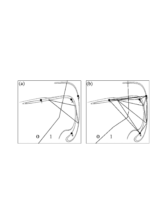
Figure 8: Inserting an orbit into the partition. (a) comparison of the topological name and of the name indicated by the current partition. In this case, the name obtained from the partition ($N_{\Gamma}(O_{3})=\overline{0111}$) matches the topological name. (b) the updated partition after the points of the period-$4$ orbit have been inserted into the list of reference points. Insertion of point # 3 increases the precision of the partition.

In the affirmative, the current partition correctly guesses the real symbolic name of the orbit (Fig. 8a): we thus add its points to the reference list, associated with the symbols indicated by the current partition. If some of the new points are closer to the border of the partition than the previous reference points, the precision of the partition is increased (Fig. 8b).

If the topological and partition names of an orbit are not consistent, we have to find the cyclic permutation of the topological name such that the insertion in the triangulation of the corresponding pairs of periodic points and symbols modifies the partition the least. To do so, we determine for each permutation which of the periodic points where the topological symbol differs from the one assigned by the current partition is most distant from the partition border, and note the corresponding distance. We then choose the cyclic permutation for which this distance is the smallest, so that the border is displaced by a small amount only.

A striking fact is that when carrying out the analysis of our sample set of orbits, there was only one orbit, the period-$23$ orbit $\langle(01)^{2}(011)^{2}(01011)^{2}(011)\rangle$, for which the second rule had to be used: the $249$ other orbits with a single topological name were already correctly encoded by the partition under construction. This orbit, and the partitions before after its insertion are shown in Fig. 9. It can be seen that the discrepancy is due to a single point which is located very close to the border of the current partition.

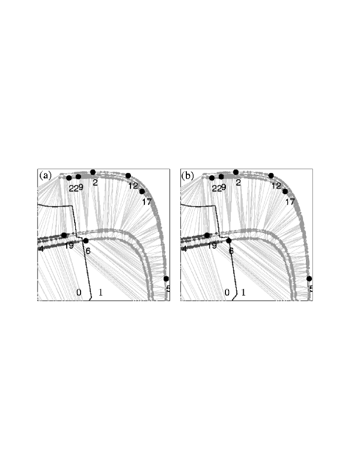
Figure 9: Comparison of the topological and partition names of the period-$23$ orbit $\langle(01)^{2}(011)^{2}(01011)^{2}(011)\rangle$. (a) The symbolic name assigned by the current partition agrees with the topological name except at point #6; (b) the updated partition after insertion of the orbit differs only slightly from the previous one, but point #6 is now on the correct side of the border.

After all orbits with a single topological name have been inserted, we obtain a partition that: (i) assigns to each of these orbits its topological name, (ii) has a simple structure, as can be seen in Fig. 10.

By using the fact that the border of this intermediate partition is localized with a very good precision, we now proceed to the orbits for which template analysis had selected several possible symbolic names, and determine which of these names is the correct one. This will allow us to further increase the resolution.

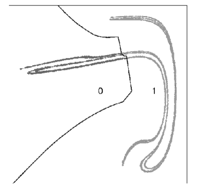
Figure 10: The partition as obtained from orbits with a single topological name. For clarity, the triangles are not shown. The large dots represent the reference points which parameterize the partition at this stage. It can be seen that the points for which the symbolic dynamical information can be unambiguously extracted cover well the attractor. This provides a graphical illustration of the observation made about Table 1, but here with orbits of periods up to 32.

3.5 Final stage of the construction

Periodic orbits with several topological names were not used in the previous step, because we had then no reason of favoring one name over the others. However, once an intermediate partition has been determined from unambiguous orbits (Fig. 10), it may be used to determine the symbols of points that are far enough from the border, if we assume that it will be only slightly modified by further refinements.

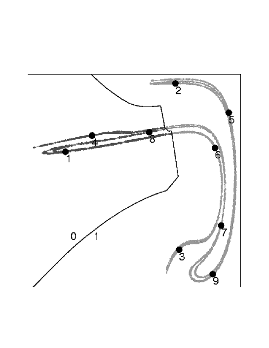
Figure 11: The periodic points of orbit #18 of Table 1, which has two possible symbolic names, are represented with the partition obtained at the end of Sec 3.4.

More precisely, consider the periodic orbit which is displayed in Fig. 11 (this is orbit #18 of Table 1). It has two possible names, namely $\mathcal{N}_{1}=\langle 010110111\rangle=\langle 0101^{2}01^{3}\rangle$ and $\mathcal{N}_{2}=\langle 010111011\rangle=\langle 0101^{3}01^{2}\rangle$. However, it can be seen that its intersections with the section plane are far from the partition border. Therefore, there is little doubt that the name indicated by the current partition, which is $N_{\Gamma}=\overline{01^{3}01^{2}01}$, is the correct one, as is confirmed by the fact that it corresponds to a cyclic permutation of $\mathcal{N}_{2}$. We can therefore assign this name to the orbit and insert it in the partition. Then, by examining Table 1, one immediately sees that since $\mathcal{N}_{2}$ has been assigned to orbit #18, it can no longer be a possible name for orbit #19. Therefore, the only remaining possible name for the latter orbit is $\mathcal{N}_{1}$, which indeed is also the one obtained from the current partition. We thus see that a consistency check (different orbits should have different names) allows us to identify the symbolic names of two orbits at once.

A more sophisticated consistency check that has to be carried after the symbolic name of an orbit has been identified is whether all the possible names of the not yet inserted orbits remain compatible with the experimental table of topological invariants. Assume that, as in the above example, the symbolic name of the $O_{i}$ orbit has just been identified as being $N_{i}=N_{\Gamma}(O_{i})$. If a possible name $\mathcal{N}_{k}(O_{j})$ of another orbit $O_{j}$ is such that the linking number $lk(N_{i},\mathcal{N}_{k}(O_{j}))$ computed from the two names does not match the measured value, $\mathcal{N}_{k}(O_{j})$ can be discarded without hesitation, as is illustrated in Table 2. This shows how enforcing simultaneously the requirements of smoothness and of topological consistency allow one to solve the ambiguities remaining after the template analysis step.

Table 2: Linking numbers of some Smale’s horseshoe orbits. Assume that the names in the first row (resp. first column) are the possible topological names of an experimental orbit $\alpha$ (resp. $\beta$), and that the linking number of these two orbits is $lk(\alpha,\beta)=66$. If the current partition can be used to show that the correct symbolic name of $\alpha$ can only be $\mathcal{N}_{2}(\alpha)$, then it follows immediately that the correct name for $\beta$ is $\mathcal{N}_{2}(\beta)$, since $lk(\mathcal{N}_{2}(\alpha),\mathcal{N}_{1}(\beta))$ does not match the experimentally measured invariant.

	$0101^{2}01^{3}=\mathcal{N}_{1}(\alpha)$	$0101^{3}01^{2}=\mathcal{N}_{2}(\alpha)$
$(01)^{3}01^{2}(01^{4})^{2}=\mathcal{N}_{1}(\beta)$	66	67
$(01)^{3}(01^{4})^{2}01^{2}=\mathcal{N}_{2}(\beta)$	67	66

For some orbits, one or more periodic points are located in a close neighborhood of the partition border. In this case, the name indicated by the partition is uncertain: some symbols may not erroneous due to the finite precision of the partition. Yet, this provisional name can be utilized to obtain the correct one, or at least to extract additional information. Indeed, if there are sequences of consecutive periodic points $O_{n}^{i},O_{n}^{i+1},\ldots,O_{n}^{i+k}$ whose symbols can be determined unambiguously, this gives us substrings $s_{i}s_{i+1}\ldots s_{i+k}$ of the correct symbolic name of this orbit. This information allows one to discard topological names that do not contain this substring. If only one topological name remains, the orbit can be inserted immediately in the partition. If there is still an ambiguity, we delay the insertion of the orbit until further information has been extracted from the other orbits.

The arguments presented above are very natural. Yet, to design a precise algorithm, we must specify what “far from the partition border” means. We thus need a precise rule to decide whether the symbol assigned by the current partition to a given point $p$ in the section plane can be trusted. We have found the following procedure to be very reliable.

We first search for all the triangles of the current triangulation whose circumcircle contains the point $p$, i.e. the triangles which would be removed if $p$ was to be inserted in the triangulation. We then examine the symbols associated with the vertices of these triangles. If all these symbols are identical, we consider that the symbol assigned to $p$ by the partition is certain. If some symbols differ, we conclude that the current partition is unreliable in the neighborhood of $p$. The rationale of this rule is that insertion of a point in the “uncertain” region defined in this way modifies the border of the partition, because it modifies the triangles whose circumcenters lie on the border.

There is however a small technical problem with this rule. Indeed it is known that the outer edges of the triangulation of a set of points compose the convex hull of this set. However, the support of the strange attractor in the section plane is generally not convex because of the folding process. Consequently, there are triangles whose vertices have different symbols merely because they are located on opposite sides of the attractor (see, e.g., Fig. 9). A direct use of the rule described above would then lead to conclude that the symbol of points contained in the circumcircles of these triangles cannot be reliably determined whereas the reference points with different symbols are far away from each other on opposite sides of the attractor.

To solve this difficulty by geometrical means, we compute a polygon that tightly encloses the support of the attractor. Triangles with different symbols are then classified according to whether the parts of their mediators belonging to the partition border have a non-empty intersection with the interior of the polygon, or not. Only the first class of triangles is used to assess the reliability of a symbol. Thus, the modified rule states that the symbol of a point cannot be reliably determined when the insertion of this point into the triangulation would modify the partition border inside the support of the strange attractor, which is illustrated in Fig. 12.

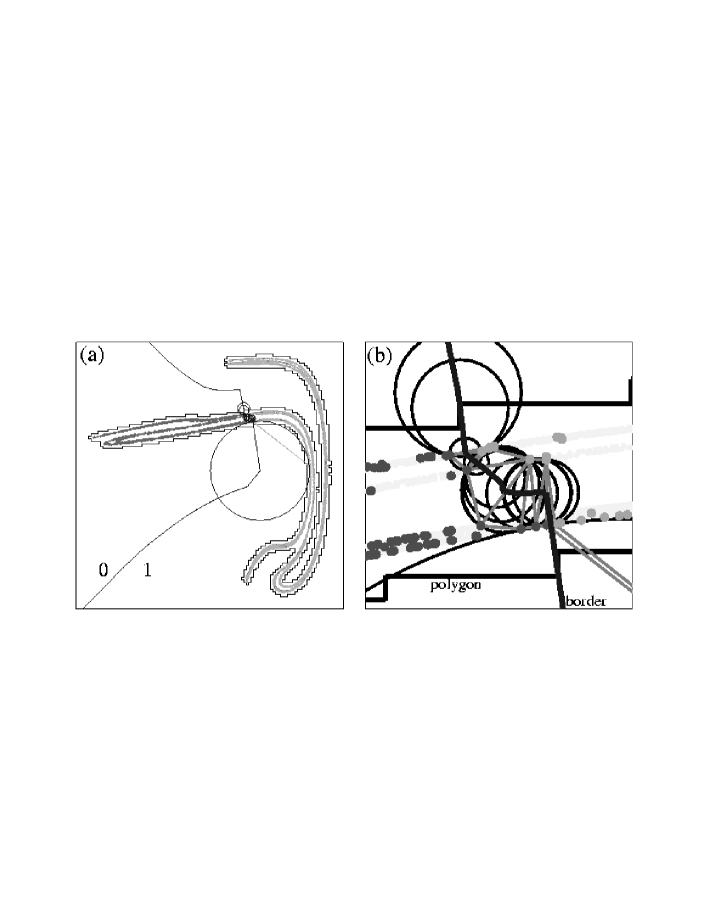
Figure 12: Regions of certain and uncertain coding. (a) a polygon providing a good approximation of the support of the strange attractor is determined. (b) Enlarged view of the border region. The uncertain region is defined to be located within the circumcircles of the triangles linking reference points with different symbols and whose mediators (which constitute the border line) lie within the shadow polygon.

To summarize, the insertion of an orbit with several possible topological names is carried out as follows. First, the symbolic encoding of this orbit by the current partition is expressed by a symbolic name $N_{c}$ with “error bars”. This symbolic name is made of the symbols $\text{``}0\text{''}$, $\text{``}1\text{''}$, …,$\text{``}n-1\text{''}$ (for points that can be unambiguously coded) and $\text{``}*\text{''}$ (for points located in the “uncertain” region). Then, we compare all cyclic permutations of each topological name to this symbolic names, with $\text{``}*\text{''}$ matching any symbol. If two or more topological names are compatible with $N_{c}$, we consider that we do not have enough information at this point to insert the orbit, but nevertheless discard the incompatible topological names. On the contrary, if only one topological name has a cyclic permutation that is compatible with $N_{c}$, we consider that it is the correct symbolic name of the orbit, and insert the orbit into the description of the partition.

Alternatively discarding names that are not compatible with the current partition and names that are no longer compatible with experimental topological invariants (as explained in Table 2) allows one to progressively insert all the orbits, so that finally each orbit is associated with a single symbolic name. The final partition, which is shown in Fig. 13, provides by construction a symbolic encoding that is both consistent with the topological structure of the set of periodic orbits and continuous (points that are close in the section plane are associated to symbolic sequences that are close in the symbol space). Given the high number of periodic orbits in our exemple, it is quite remarkable that the simple rules we have followed naturally select a single name for each orbit: this supports the existence of a well-defined symbolic encoding.

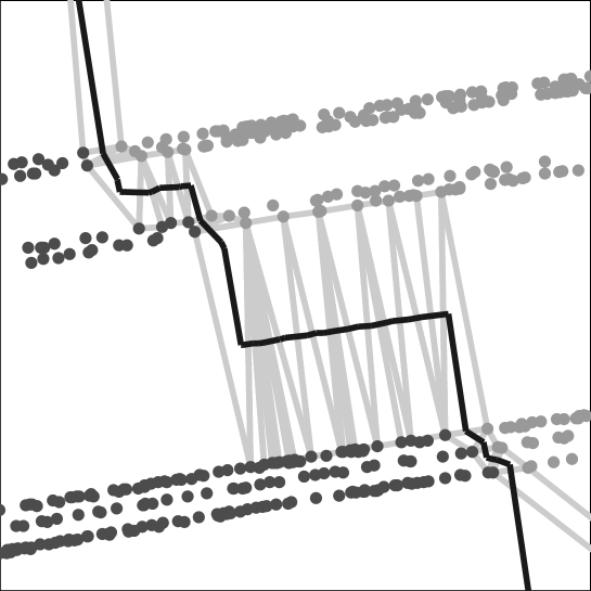
Figure 13: Enlarged view of the border of the final partition, obtained when all the periodic orbits have been inserted (the large-scale structure is virtually identical to that shown in Fig. 10). The width of the represented box is $5\times 10^{-2}$ in units of the attractor width and the linewidth used to draw the border line and the reference points is $5\times 10^{-4}$.

Note that the rule we have defined to assess the reliability of the symbol associated to a point can be interpreted as an interpolation problem. Indeed, Delaunay triangulations are routinely used to interpolate the value of a function at an arbitrary point $p$ from known values at the sites of the triangulation. There are essentially two methods to do so. The first averages appropriately the values at the three vertices of the triangle that contains $p$. The second utilizes the vertices of all the triangles whose circumcircle contains $p$, and is called “natural neighbor interpolation” [69].

Thus, it appears that our procedure, which we initially derived from the heuristic argument presented above, is based on the latter. When the result of the interpolation is exactly one of the $n$ possible symbols (because all neighboring vertices have the same symbol), the result is considered as certain. When the interpolation yields a value that is intermediate between two symbols (some neighboring vertices have different vertices), the encoding is considered as uncertain. It is interesting to note that an earlier version of our algorithm based on the first interpolation method did not converge in some cases because some periodic points were incorrectly classified as certain, leading to inconsistencies when inserting the remaining orbits. This is because the reference point which is closest to $p$ need not be a vertex of the triangle containing $p$ whereas it is known that it is a vertex of one of the triangles whose circumcircle contains $p$.

In conclusion, it results that simple rules can be used to construct a partition of the section plane using the information provided by (i) the topological invariants of the unstable periodic orbits, and (ii) their positions in the section plane. We have seen that this algorithm yields partitions that have a very simple structure, and therefore encode points with high reliability, except in a very small region around the border of the partition.

3.6 Increasing the resolution of the partition

In describing our algorithm in the previous sections, our aim was to show that no inconsistency was found even when shadowing all the trajectories on the attractor with a high resolution, i.e., that it was possible to assign unambiguously to every orbit a distinct symbolic name compatible with its topological invariants. To this end, we utilized a set of orbits that provided an uniform cover of the attractor. For practical applications, however, a high-resolution cover is only needed in a small neighborhood of the border of the partition. To achieve a high precision at the lowest cost, we have therefore modified our method as follows.

The procedure was split into two stages. First, an approximate partition is determined using a set of orbits of limited period providing a cover of moderate resolution. This allows one to bracket the position of the border with reasonable accuracy. Using this information, a second set of periodic orbits is selected so that it provides a cover of the attractor with high resolution in the neighborhood of the border, more precisely inside the circumcenters of the triangles enclosing it, and with moderate resolution elsewhere.

We then apply to the latter set a slightly modified version of the algorithm described in the previous sections. Indeed, we have observed that obtaining a high-resolution cover in the critical region requires using orbits of very high period, especially when there are many forbidden sequences in the symbolic dynamics. This does not induce additional difficulties in the first steps of the procedure because (i) high-period orbits localized near the border of the partition are marginally unstable, which makes their detection relatively easy, (ii) topological invariants are expressed by integer numbers and can therefore be reliably computed for orbits of very large periods.

In fact, the limiting step is the search for possible symbolic names using template analysis. Indeed, this search requires a considerable amount of computing time because the number of symbolic names of length $p$ increases exponentially with $p$, especially when the symbolic dynamics is based on three or more symbols. For a two-symbol dynamics, the symbolic names of orbits with periods up to 32 can be determined in a reasonable amount of computing time, while in the three-symbol case, a direct search is practically limited to orbits of period lower than 20.

We thus restrict this search to the orbits up to a certain period. An intermediate partition is built from these orbits, and is utilized to list for the remaining higher-period orbits the symbolic names which (i) are compatible with this partition, as explained in Sec. 3.5, and (ii) correctly predict the topological invariants of these higher-period orbits.

Once a list of possible names has been so obtained for each orbit in the final set, the analysis proceeds as in Sec. 3. It should be stressed that this procedure is entirely equivalent to the one described in Secs. 3.3 to 3.5 where all the topological names are determined before trying to build the partition: we simply apply the selection criteria in a different order.

With this modified algorithm, and a final set of 750 orbits of periods up to 64, we have obtained for the chaotic attractor of Fig. 2 a partition whose border is bracketed with a resolution that is almost everywhere significantly below 0.01% of the attractor width (see Fig. 14b). Note that the same precision could be clearly be obtained at a lower cost by using a significantly smaller number of periodic orbits. Indeed, it can be seen in Fig. 14a that many triangles connecting two leaves of the attractor are in fact not essential for localizing precisely the border, but were nevertheless considered by our algorithm to belong to the border neighborhood. The many periodic points associated with these triangles (the detection code is in high-resolution mode in this region) could therefore be discarded from the set of orbits without modifying the result.

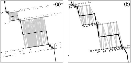
Figure 14: (a) Enlarged view of the border of the partition obtained using a high-resolution cover of the border region by periodic points (the size of the represented box is the same as in Fig. 13, i.e., $5\times 10^{-2}$ in units of the attractor width). The triangles shown are those defining the partition border inside the shadow polygon. Note the high density of periodic points associated with these triangles due to the design of our selection algorithm. (b) Enlarged view of the small square of size $5\times 10^{-3}$ displayed in the left picture. The linewidth used to draw the border line and the periodic points is $5\times 10^{-5}$.

It should be noted that such a precision is several orders of magnitude higher than is needed for practical purposes. In fact, as we will show in the second part of this work [16], one has to compare trajectories whose symbolic sequences have common substrings of more than 60 symbols to observe an effect due to the error in the location of the border. Nevertheless, this example has allowed us to verify the robustness of our algorithm down to very small scales. Furthermore, it provides us with a test case which we will use in the second part of this work to give evidence that our approach is consistent with methods based on homoclinic tangencies.

4 Conclusion and perspectives

Our primary goal in showing that template analysis can be used to obtain high-resolution partitions in numerical simulations was to give strong evidence of the validity of the approach proposed in [15]. A first result is the successful outcome of an intensive check of the validity of template analysis: even when using large sets of UPO of high periods, we could always find a global projection on a simple branched manifold that preserves the topological invariants. Although the application of template theory to real, nonhyperbolic, attractors is still lacking a rigorous foundation, the present work gives further evidence that it accurately describes the geometric structure of an attractor down to very small scales. Although embedded in a nonhyperbolic attractor, the UPO appear to be organized as in the hyperbolic limit, and constitute an hyperbolic set which approximates well the strange attractor.

The foundation of this work is the fact that the knot invariants of an unstable periodic orbit carry precise information about its symbolic dynamics. Building on this idea, we have described an algorithm to construct generating partitions of a strange attractor. It combines information (i) from the topological invariants of UPO embedded in it, and (ii) from their location in a section plane, and is designed so as to yield encodings that are continuous (sequences associated to neighboring points should be close in symbol space). These basic ingredients ensure that the resulting encodings are compatible with those valid in the one-dimensional and hyperbolic limits, and that they are dynamically relevant.

In our algorithm, a partition is described by a list of reference points, whose associated symbols are given. To perform a symbolic encoding, points in the section plane are associated with the symbol carried by the closest reference point. This allows us to use simple geometrical tools such as Delaunay triangulations. Starting from an initial configuration based on the lowest-period orbits, the accuracy of the partition is progressively improved by adding periodic points of increasing period to the list of reference points in a way that preserves the simplicity of the partition and topological consistency.

Following this procedure, we have obtained partitions that have a simple structure, yet reproduce the symbolic information extracted from topological analysis: the unique symbolic name that is eventually assigned to each periodic orbit is intimately related to its topological structure, and hence to its genealogy [8, 19, 70, 71]. Had we faced an inconsistency at some stage of the construction, we would have been forced to conclude that there was a fundamental flaw in our hypotheses. This was not the case neither in the example we considered in this paper (we recall that it involved a set of 1594 periodic orbits, whose topological information was contained in about $4.4\times 10^{6}$ integer numbers), nor in others that we have studied.

The present results call for further investigations in several directions. First, we have to verify more extensively the relevance of the obtained encodings, even if this should be guaranteed by the consistency checks built into our algorithm. We do so in the second part of this work [16], where in particular we show that the border of the high-resolution partition displayed in Fig. 14 follows very accurately a line of homoclinic tangencies, thus proving the equivalence of the two approaches. We also give in [16] additional evidence of the relevance of our algorithm by verifying (i) that encodings obtained from different initial partitions are dynamically equivalent, (ii) that accurate estimates of the metric entropy can be computed from the probabilities of symbolic sequences, and (iii) that symbolic sequences of increasing length select regions of decreasing diameter in the section plane.

The robustness of our method with respect to noise should also be more precisely studied. While template analysis behaves well in this context, it would be desirable to quantify precisely the highest noise level that is acceptable for extracting meaningful results. To achieve this, a characterization of simulated time series contaminated by various amounts of noise, and where UPO are detected from close returns, is required.

Similarly, the independence of symbolic encodings with respect to changes in parameter values should be carefully checked: in this work, we have determined generating partitions only at a given set of parameters. While it is obvious that the orbits with a unique topological name will always be assigned the same name on their whole domain of existence, we have to verify that this also holds for the higher-period orbits whose identification is completed during the construction of the partition.

This check will be absolutely required to be able to state with reasonable confidence that the discontinuous changes in encodings observed in orientation-reversing maps [36, 37] cannot occur in orientation-preserving ones. The contradiction between the phenomena reported in Refs [36, 37] and constraints obeyed by orientation-preserving maps, which is unveiled by simple topological arguments (see Sec. 2.4), certainly deserves further investigations in its own. In this context, note that although knot invariants are defined for orbits of a three-dimensional flow, the techniques described here can easily be applied to invertible orientation-preserving two-dimensional maps, such as the Ikeda map or the Hénon map with positive Jacobian. One can either construct a suspension of the map satisfying the uniqueness theorem, or utilize the powerful techniques presented in Refs. [72], where it was shown that the braid type of an orbit can be directly determined from its intersections with a surface of section, up to a global torsion.

In the case of infinitely dissipative system, the relevant part of the triangulation essentially consists of two periodic points located on opposite sites of the border. In the mildly dissipative examples we have considered in this work, the triangles enclosing the border involve a significantly higher number of periodic points. It would be highly interesting to determine whether these borderline periodic points are directly related to the symbolic sequences defining the “pruning front” in symbol plane [21]. Another point worth investigating is whether these orbits belong to a basis set (in orbit forcing theory [70, 71, 8], a basis set is a small set of periodic orbits whose existence can be shown to force the existence of all the other orbits embedded in the attractor).

On the experimental side, we intend to apply very soon the algorithm described here to a weakly dissipative experimental system, namely a pump-modulated Nd:YAG laser. Indeed, the first experimental topological encoding was obtained for a system which was relatively dissipative (a CO₂ laser with modulated losses), even though its return map could not be described by a well-defined one-dimensional map on a wide range of parameters [15].

To conclude, we would like to comment on the links that exist between the topological approach we have discussed in this work and the classical one based on homoclinic tangencies, although they seem to have no common ground at first glance. As we will show in [16], these two methods yield results that are equivalent, and thus must correspond to different views of a single structure. In fact, both ultimately rely on the fact that a chaotic invertible return map is a diffeomorphism organized by underlying singularities.

To have these singularities appear undressed in the form of homoclinic tangencies, it is necessary to iterate the return map an infinite number of times. In doing so, however, one not only recovers the organizing singularities, but also an infinite number of copies of them. As a result, there is a fundamental ambiguity in the choice of the homoclinic tangencies defining the partition. This can only be solved by searching directly in the time-one map the singularities that are hidden in it.

The Birman-Williams construction for hyperbolic systems provides a deep answer to this problem. In the case of the horseshoe map, the one-dimensional return map of the semi-flow defined on the branched manifold features explicitly the fold singularity that is the backbone of the two-dimensional horseshoe map, as well as any three-dimensional suspension of it. This seems to indicate that the structure of an invertible return map is inherited from a lower-dimensional non-invertible map carrying the singularities that organize the dynamics [73].

Our approach does not try to construct directly such a singular map. Rather, it focuses on the “track” of the one-dimensional singularity, i.e., on points of the section plane that are projected onto this singularity, if a “projection” similar to the Birman-Williams one can be given a well-defined meaning.

The initial partition based on a few low-period orbits separates their periodic point according to how they should located on an underlying singular map, and in a sense provides a rough geometric modeling of such a map. The hierarchical refinement of the partition carried out by progressively inserting higher-order orbits can be viewed as a means to ensure that “iterates” of this singular map converge to iterates of the invertible return map. In this way, the singularities which appear in the infinitely iterated return map are eventually localized while keeping the geometrical description close to that of the time-one map. This allows one to extract information from the whole phase space without having to approach too closely the noise-perturbed singularities.

This discussion makes it easier to understand why mathematical tools that are intimately linked to the theory of one-dimensional symbolic dynamics are so perfectly suited to the study of two-dimensional dynamics. One key to this apparent paradox is that unstable periodic orbits, among all other trajectories in the attractor, have a very distinctive property: their forward symbolic sequence is uniquely determined from their backward one, and vice versa. From a symbolic dynamical point of view, periodic orbits are thus one-dimensional objects intertwined with the fully two-dimensional chaotic trajectories, which makes it possible to extend information extracted from the former to the latter.

The bridge between the non-invertible and the invertible dynamics is provided by the knot invariants of the UPO, which indicate how the latter should be laid on the domain of the underlying one-dimensional map without having to construct it explicitly. These invariants thus play a role that is not unlike the conserved quantities or symmetries that have proved so immensely useful in many fields of physics. To extend topological coding to higher-dimensional chaos, and understand its singularity structure, we thus now have to find what are in this case the appropriate invariant quantities.

References

- [1] J. Guckenheimer and P. J. Holmes, Nonlinear Oscillations, Dynamical Systems and Bifurcations of Vector Fields (Springer Verlag, Berlin, 1983).
- [2] A. Katok and B. Hasselblatt, Introduction to the Modern Theory of Dynamical Systems (Cambridge University Press, Cambdrige, 1995).
- [3] Hao Bai-Lin, Elementary Symbolic Dynamics and Chaos in Dissipative Systems (World Scientific, Singapore, 1989).
- [4] R. Badii and A. Politi, Complexity : Hierarchical structures and scaling in physics, Vol. 6 of Cambridge Nonlinear Science Series (Cambridge University Press, Cambridge, 1997).
- [5] S. Hayes, C. Grebogi, and E. Ott, “Communicating with chaos”, Phys. Rev. Lett. 70, 3031–3034 (1993).
- [6] S. Hayes, C. Grebogi, E. Ott, and A. Mark, “Experimental control of chaos for communication”, Phys. Rev. Lett. 73, 1781–1784 (1994).
- [7] P. Grassberger and H. Kantz, “Generating partitions for the dissipative Hénon map.”, Phys. Lett. A 113, 235–238 (1985).
- [8] R. Gilmore, “Topological analysis of chaotic dynamical systems”, Rev. Mod. Phys. 70, 1455–1530 (1998).
- [9] N. B. Tufillaro, T. A. Abbott, and J. P. Reilly, An Experimental Approach to Nonlinear Dynamics and Chaos (Addison-Wesley, Reading, 1992).
- [10] H. G. Solari, M. A. Natiello, and G. B. Mindlin, Nonlinear Dynamics: a Two-Way Trip from Physics to Math (IOP Publishers, London, 1996).
- [11] G. B. Mindlin, X.-J. Hou, H. G. Solari, R. Gilmore, and N. B. Tufillaro, “Characterization of strange attractors by integers”, Phys. Rev. Lett. 64, 2350–2353 (1990).
- [12] G. B. Mindlin, H. G. Solari, M. A. Natiello, R. Gilmore, and X.-J. Hou, “Topological analysis of chaotic time series data from Belousov-Zhabotinski reaction”, J. Nonlinear Sci. 1, 147–173 (1991).
- [13] J. S. Birman and R. F. Williams, “Knotted periodic orbits in dynamical systems I: Lorenz’s equations”, Topology 22, 47–82 (1983).
- [14] R. W. Ghrist, P. J. Holmes, and M. C. Sullivan, Knots and Links in Three-Dimensional Flows, Vol. 1654 of Lecture Notes in Mathematics (Springer, Berlin, 1997).
- [15] M. Lefranc, P. Glorieux, F. Papoff, F. Molesti, and E. Arimondo, “Combining topological analysis and symbolic dynamics to describe a strange attractor and its crises”, Phys. Rev. Lett. 73, 1364–1367 (1994).
- [16] J. Plumecoq and M. Lefranc, “From template analysis to generating partitions II: checking the validity of the method” (unpublished).
- [17] H. D. Abarbanel, R. Brown, J. J. Sidorowich, and L. S. Tsimring, “The analysis of observed chaotic data in physical systems”, Rev. Mod. Phys. 65, 1331–1392 (1993).
- [18] P. J. Holmes, “Knotted periodic orbits in suspensions of Smale’s horseshoe: period multiplying and cabled knots.”, Physica D 21, 7–41 (1986).
- [19] P. J. Holmes, in New directions in dynamical systems, edited by T. Bedford and J. Swift (Cambridge University Press, Cambridge, 1988), pp. 150–191.
- [20] P. Grassberger, H. Kantz, and U. Moenig, “On the symbolic dynamics of the Hénon map”, J. Phys. A 22, 5217–5230 (1989).
- [21] P. Cvitanovic, G. H. Gunaratne, and I. Procaccia, “Topological and metric properties of Hénon-type strange attractors.”, Phys. Rev. A 38, 1503–1520 (1988).
- [22] G. D’Alessandro, P. Grassberger, S. Isola, and A. Politi, “On the topology of the Hénon map”, J. Phys. A: Math. Gen. 23, 5285–5294 (1990).
- [23] F. Giovannini and A. Politi, “Homoclinic tangencies, generating partitions and curvature of invariant manifolds”, J. Phys. A: Math. Gen. 24, 1837–1848 (1991).
- [24] L. Jaeger and H. Kantz, “Structure of generating partitions for two-dimensional maps”, J. Phys. A: Math. Gen. 30, L567–576 (1997).
- [25] Z.-B. Wu, “Symbolic dynamics analysis of chaotic time-series with a driven frequency”, Phys. Rev. E 53, 1446–1452 (1996).
- [26] L. Jaeger and H. Kantz, “Homoclinic tangencies and non-normal Jacobians - effects of noise in nonhyperbolic chaotic systems”, Physica D 105, 79–96 (1997).
- [27] R. Gilmore, Catastrophe Theory for Scientists and Engineers (Wiley, New York, 1981), reprinted by Dover, New York, 1993.
- [28] H. G. Solari and R. Gilmore, “Relative rotation rates for driven dynamical systems”, Phys. Rev. A 37, 3096–3109 (1988).
- [29] L. Flepp, R. Holzner, E. Brun, M. Finardi, and R. Badii, “Model identification by periodic-orbit analysis for NMR-laser chaos”, Phys. Rev. Lett. 67, 2244–2247 (1991).
- [30] M. Finardi, L. Flepp, J. Parisi, R. Holzner, R. Badii, and E. Brun, “Topological and metric analysis of heteroclinic crisis in laser chaos”, Phys. Rev. Lett. 68, 2989–2991 (1992).
- [31] R. Badii, E. Brun, M. Finardi, L. Flepp, R. Holzner, J. Parisi, C. Reyl, and J. Simonet, “Progress in the analysis of experimental chaos through periodic orbits”, Rev. Mod. Phys. 66, 1389–1415 (1994).
- [32] D. Auerbach, P. Cvitanovic, J.-P. Eckmann, G. Gunaratne, and I. Procaccia, “Exploring chaotic motion through periodic orbits”, Phys. Rev. Lett. 58, 2387–2389 (1987).
- [33] D. Lathrop and E. J. Kostelich, “Characterization of a strange attractor by periodic orbits”, Phys. Rev. A 40, 4028–4031 (1989).
- [34] E. Ott, C. Grebogi, and J. Yorke, “Controlling chaos”, Phys. Rev. Lett. 64, 1196–1199 (1990).
- [35] L. H. Kaufmann, Knots and Physics (World Scientific, Singapore, 1991).
- [36] K. Hansen, “Remarks on the symbolic dynamics for the Hénon map”, Phys. Lett. A 165, 100–104 (1992).
- [37] F. Giovannini and A. Politi, “Generating partitions in H non-type maps”, Phys. Lett. A 161, 332–336 (1992).
- [38] J. Birman and R. Williams, “Knotted periodic orbits in dynamical systems II: knot holders for fibered knots”, Cont. Math. 20, 1–60 (1983).
- [39] P. J. Holmes and R. F. Williams, “Knotted periodic orbits in suspensions of Smale’s horseshoe: torus knots and bifurcation sequences.”, Arch. Rat. Mech. Anal. 90, 15–194 (1985).
- [40] P. J. Holmes, “Knotted periodic orbits in suspensions of annulus maps.”, Proc. Roy. Soc. Lond. A411, 351–378 (1987).
- [41] P. J. Holmes, “Knotted period orbits in suspensions of Smale’s horseshoe: extended families and bifurcation sequences”, Physica D 40, 42–64 (1989).
- [42] N. B. Tufillaro, R. Holzner, L. Flepp., R. Brun, M. Finardi, and R. Badii, “Template analysis for a chaotic NMR laser”, Phys. Rev. A 44, R4786–4788 (1991).
- [43] F. Papoff, A. Fioretti, E. Arimondo, G. B. Mindlin, H. G. Solari, and R. Gilmore, “Structure of chaos in the laser with a saturable absorber”, Phys. Rev. Lett. 68, 1128–1131 (1992).
- [44] A. Fioretti, F. Molesti, B. Zambon, E. Arimondo, and F. Papoff, “Topological analysis of laser with saturable absorber in experiments and models”, Int. J. Bifurcation Chaos Appl. Sci. Eng. 3, 559–564 (1993).
- [45] M. Lefranc and P. Glorieux, “Topological analysis of chaotic signals from a CO2 laser with modulated losses”, Int. J. Bifurcation Chaos Appl. Sci. Eng. 3, 643–649 (1993).
- [46] T. Braun, R. R. B. Correira, and N. Altmann, “Topological model of homoclinic chaos in a glow discharge”, Phys. Rev. E 51, 4165–4168 (1995).
- [47] C. Letellier, L. L. Sceller, P. Dutertre, G. Gouesbet, Z. Fei, and J. L. Hudson, “Topological characterization and global vector field reconstruction of an experimental electrochemical system”, J. Phys. Chem. 99, 7016–7027 (1995).
- [48] N. B. Tufillaro, P. Wyckoff, R. Brown, T. Schreiber, and T. Molteno, “Topological time series analysis of a string experiment and its synchronized model”, Phys. Rev. E 51, 164–174 (1995).
- [49] C. Letellier, G. Gouesbet, and N. F. Rulkov, “Topological analysis of chaos in equivariant electronic circuits”, Int. J. Bifurcation Chaos Appl. Sci. Eng. 6, 2531–2555 (1996).
- [50] G. Boulant, M. Lefranc, S. Bielawski, and D. Derozier, “Horseshoe templates with global torsion in a driven laser”, Phys. Rev. E 55, 5082–5091 (1997).
- [51] G. Boulant, S. Bielawski, D. Derozier, and M. Lefranc, “Experimental observation of a chaotic attractor with a reverse horsehoe topological structure”, Phys. Rev. E 55, R3801–3804 (1997).
- [52] J. W. L. McCallum and R. Gilmore, “A geometric model for the Duffing oscillator”, Int. J. Bifurcation Chaos Appl. Sci. Eng. 3, 685–691 (1993).
- [53] R. Gilmore and J. W. L. McCallum, “Structure in the bifurcation diagram of the Duffing oscillator”, Phys. Rev. E 51, 935–956 (1995).
- [54] C. Letellier, P. Dutertre, and G. Gouesbet, “Characterization of the Lorenz system, taking into account the equivariance of the vector field”, Phys. Rev. E 49, 3492–3495 (1994).
- [55] C. Letellier, P. Dutertre, and B. Maheu, “Unstable periodic orbits and templates of the Rössler system: toward a systematic topological characterization”, Chaos 5, 271–282 (1995).
- [56] N. B. Tufillaro, “Braid analysis of a bouncing ball”, Phys. Rev. E 50, 4509–4522 (1994).
- [57] C. Letellier, G. Gouesbet, F. Soufi, J. R. Buchler, and Z. Kolláth, “Chaos in variable stars: topological analysis of W Vir model pulsations”, Chaos 6, 466–476 (1996).
- [58] G. Boulant, M. Lefranc, S. Bielawski, and D. Derozier, “A non-horseshoe template in a chaotic laser model”, Int. J. Birfurcation Chaos Appl. Sci. Eng. 8, 965–975 (1998).
- [59] R. Gilmore, R. Vilaseca, R. Corbalan, and E. Roldan, “Topological analysis of chaos in the optically pumped laser”, Phys. Rev. E 55, 2479–2487 (1997).
- [60] P. Melvin and N. B. Tufillaro, “Templates and framed braids”, Phys. Rev. A 44, 3419–3422 (1991).
- [61] M. Lefranc (unpublished).
- [62] J. R. Tredicce, F. T. Arecchi, G. P. Puccioni, A. Poggi, and W. Gadomski, “Dynamics behavior and onset of low-dimensional chaos in a modulated homogeneously broadened single-mode laser: experiments and theory”, Phys. Rev. A 3, 2073–2081 (1986).
- [63] D. Dangoisse, P. Glorieux, and D. Hennequin, “Chaos in a CO2 laser with modulated parameters: experiments and numerical simulations”, Phys. Rev. A 36, 4775–4791 (1987).
- [64] F. Aurenhammer, “Voronoi diagrams — a survey of a fundamental geometric data structure”, ACM Computing Surveys 23, 345–405 (1991).
- [65] F. P. Preparata and M. I. Shamos, Computational Geometry: An Introduction (Springer, Berlin, 1985).
- [66] A. Okabe, B. Boots, and K. Sugihara, Spatial Tessellations: Concepts and Applications of Voronoi Diagrams (Wiley, Chichester, England, 1992).
- [67] D. F. Watson, “Computing the -dimensional Delaunay tesselation with application to Voronoi polytopes”, The Computer J. 24, 167–172 (1981).
- [68] J.-D. Boissonat and M. Teillaud, in Proc. 2nd Annu. ACM Sympos. Comput. Geom. (ACM, New York, 1986), pp. 260–268.
- [69] D. F. Watson, “Natural neighboring sorting”, The Australian Computer J. 17, 189–193 (1985).
- [70] G. B. Mindlin, R. Lopez-Ruiz, H. G. Solari, and R. Gilmore, “Horseshoe implications”, Phys. Rev. E 48, 4297–4304 (1993).
- [71] T. Hall, “Weak universality in two-dimensional transitions to chaos”, Phys. Rev. Lett. 71, 58–61 (1993).
- [72] H. G. Solari, M. A. Natiello, and M. Vázquez, “Braids on the Poincaré section: a laser example”, Phys. Rev. E 54, 3185–3195 (1996).
- [73] R. Gilmore, in Applications of Soft Computing, Vol. 3165 of Proc. SPIE, edited by B. Bosacchi, J. C. Bezdek, and D. B. Fogel (SPIE, Bellingham, 1997), pp. 243–257.