Inhomogeneous turbulence in the vicinity of a large scale coherent vortex

Abstract

We study the statistics of turbulent velocity fluctuations in the neighbourhood of a strong large scale vortex at very large Reynolds number. At each distance from the vortex core, we observe that the velocity spectrum has a power law “inertial range” of scales and that intermittency – defined as the variation of the probability density function (PDF) of velocity increments as the length of the increment is varied – is also present. We show that the spectrum scaling exponents and intermittency characteristics vary with the distance to the vortex. They are also influenced by the large scale dynamics of the vortex.

1 Introduction

Much efforts have been devoted to the study of high Reynolds number turbulence, assuming the properties of local homogeneity and isotropy. Under these assumptions it has been shown [1] that, in between the integral scale at which energy is fed into the flow and the dissipative scale at which viscosity smoothes out the velocity gradients, there exists an “inertial range” where: (i) the velocity spatial power spectrum follows a power law $E(k)\sim\epsilon^{2/3}k^{-5/3}$, (ii) the energy transfer rate $\epsilon$ is related to the third order structure function $S_{3}(r)=\langle\delta u^{3}(r)\rangle=-\frac{4}{5}\epsilon r$. The first point has been verified experimentally in numerous experiments and constitutes the main success of Kolmogorov’s K41 mean field theory [2]. The second point is generally admitted although experimental verifications are rarer [3]. In addition, it has been observed that the probability distribution of the amplitudes of velocity increments depends on the width of the increment. It varies from a gaussian PDF at integral scale to the development of stretched exponential tails at the smallest scales. This feature defines intermittency, and traces back to the non-uniformity in space of the energy transfer rate. These three observations are the building blocks of the studies of homogeneous, isotropic tubulence (HIT).

It is the aim of our work to study experimentally how these observations are modified in a situation of inhomogeneous turbulence. Partial studies have been made near weak vortices [4], in inhomogeneous wakes [5, 6] or near a boundary layer [7, 8]. Here we study turbulence in the vicinity of a very intense large scale vortex. Our motivations are twofold: first, most high Reynolds numbers flows are inhomogenous and the question of the “universality” of the features of HIT should be addressed. A second motivation is that it has been proposed that such coherent structures play a significant role in the statistical properties of turbulence [9, 10, 11, 12].

2 Experimental set-up and measurements

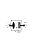
The experimental apparatus and measurement techniques are those described in [13]. A strong axial vortex is formed in the gap between two corotating disks – fig. 1. The control parameters of the flow are the disks angular velocities: $\Omega_{1}$, $\Omega_{2}$, and the mean integral Renolds number: $Re={R^{2}\sqrt{\Omega_{1}^{2}+\Omega_{2}^{2}}}/{\nu}.$ Essentially two regimes are observed. The first one, hereafter labeled (GR), is when $\Omega_{1}\sim\Omega_{2}$: the core of the flow has a strong global rotation and a stable large scale axial vortex is present. On the other hand, when one disk rotates at a much faster rate than the other, the flow is dominated by differential rotation; a strong axial flow is produced and one observes intermittent sequences of formation and bursting of large scale axial vortices [13] – in the following, we label (DR) this regime. In each case, the integral Reynolds number of the flow exceeds $5\,.10^{5}$ so that the flow is ‘turbulent’.

Fig. 1.–: Experimental setup. The fluid is confined in a cylindrical vessel of height 40 cm and radius 11.7 cm. The disks, of radius $R=9.8$ cm are set a distance $H=30$ cm apart. They are driven by two d.c. motors whose rotation rates $\Omega_{1},\Omega_{2}$ are adjustable in the range $[15,45]$ Hz. The hot-film probe is located just above the midplane, at variable distance $r$ from the axis of rotation.

Local velocity measurements are performed as in [13]. The hot-film probe is set parallel to the axis of rotation, so that it measures $u_{r\theta}=\sqrt{u_{r}^{2}+u_{\theta}^{2}}$ (here, $(r,\theta,z)$ are the conventional cylindrical coordinates with $z$ parallel to the rotation axis). The sampling frequency $Fs$ is 78125 Hz for measurements in the (DR) regime and $39062.5$ Hz in (GR) – In each case, at least $10^{7}$ data points are collected. We stress that although the flow has in most locations a well defined mean value $\overline{u}$ of the velocity $u_{r\theta}$ and fluctuation levels $u_{\rm rms}$ comparable or less to thoses reported in jet turbulence, we do not attempt to use and justify a ‘Taylor hypothesis’ here and we analyse our result as time series.

3 Spectra

A first question regarding such a turbulence concerns the range of scales of motion and the energy distribution among them. In fig. 2 we show the power spectra of velocity time series recorded at different distances from the rotation axis. It can be observed, as a first sign of the flow inhomogeneity, that the spectra depend very much on the location of the probe and on the flow configuration.

Fig. 2.–: Power spectra of velocity times series recorded at distances $(0$, $0.5$, $1$, $1.5$, $2$, $2.5$, $3$, $3.5$, $4$, $4.5$, $5.5)$ cm from the rotation axis. (a): $\Omega_{1}=\Omega_{2}=30$ Hz; (b) : $\Omega_{1}=40$ Hz, $\Omega_{2}=12$ Hz.

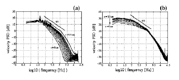
In all cases, we observe the existence of an ‘inertial range’ $\omega\in[\omega_{I},\omega_{T}]$ where the spectrum follows a power law $E(\omega)\propto\omega^{-\alpha}$. However both the range $\omega_{I}/\omega_{T}$ and the exponent $\alpha$ vary.
- In (GR), $\alpha$ increases from about 1.65 in the outer region, to 2.50 at the rotation axis; meanwhile the scaling domain is also reduced. A more detailed analysis of the spectra shows that the energy in the larges scales remains approximately constant while both the frequency and the energy at the end of the ’inertial range’ decrease with $r$. As a result, the proximity of the stable vortex structure reduces the range of scales of the turbulent motion and their energy content. This is consistent with earlier findings [14, 15] which have shown that global rotation tends to decrease the intensity of small scales motion.
- In (DR), $\alpha$ decreases from again about 1.65 in the outer region, to $1.1$ at the rotation axis. The scaling range does not vary. Here, one observes that the energy in the dissipative region is almost independent of the position $r$ of measurement. It is the energy measured in the large scales that decreases with $r$.

We thus find that the dynamics of the large scales influences the entire range of scales. It is surprising to observe that some self-similarity is retained since the spectra follow a power law (most curves exhibit almost a decade of scaling behaviour): there is no scale separation where one would observe the pathologies of the injection at large scales and where the turbulence would recover the characteristics of HIT at small scales.

4 Third order structure function

The energy transfer across the scales is usually illustrated by the behaviour of the third order structure function. In HIT, this is justified by the Kármán-Howarth relationship. But an anistropic equivalent can be established [2]. We show in fig. 3 the evolution of the third order moment of the velocity increments $S_{3}(\tau)=\langle\left(u(t)-u(t+\tau)\right)^{3}\rangle_{t}$, computed at different distances from the rotation axis.
- In (GR), we observe that in the outer region, $S_{3}(\tau)$ is a negative, bell-shaped curve. Negative values of the skewness indicate that the cascade proceeds in the forward direction, from the large scales to the dissipative ones, as in HIT. At such limited Reynolds numbers, one cannot expect a plateau in plots of $S_{3}(\tau)/\tau$ (even less with value $-4/5$), but the maximum of $|S_{3}(\tau)/\tau|$ is consistent with the value of the power consumption per unit mass $\epsilon$, measured from the electric consumption of the motors [16]. On the contrary going towards the axis the amplitude of $S_{3}(\tau)$ diminishes rapidly. Near the vortex core, the skewness eventually becomes positive in an intermediate range of increments. This indicates that the cascade to small scales is first reduced, and then reversed by the influence of the coherent rotation of the vortex. Energy is accumulated in the large scale where it stabilizes the dynamics of the large scale vortex.

Fig. 3.–: Evolution with increment length of the third order moment of the velocity. (a): (GR) regime; (b): (DR) regime. $S_{3}(\tau)$ is computed at distances $r=0.5(\circ),\;1.5(\Diamond),\;2.5(\Box),\;3.5(\triangle),\;4.5(\star)$ cm from the axis. The horizontal axis is in units of the sampling frequency.

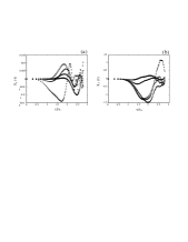
- This picture is quite different in the irregular (DR) regime. There, except at the rotation axis, the skewness has the behaviour traditionnally observed in HIT. The cascade proceeds forward; the maximum shows little variation with the location of the probe and has a value which is, again, consistent with the motors power consumption. At the axis, $S_{3}(\tau)$ drops suddenly; even its sign becomes unclear and it may even be slightly positive in a range of scales.

Altogether, the analysis of the third order moment shows that the structure and dynamics of the flow at large scale strongly influences the entire energy transfer across the scales.

5 Intermittency

A first observation is that intermittency is always present, regardless of the flow regime and probe location. Indeed, for every measurement, the PDFs of velocity increment change from a quasi-gaussian shape at integral scale to the development of stretched exponential tails at small scales, see fig.4 (the PDFs shown in this figure are for signed quantities).

Fig. 4.–: Evolution with increment length of PDFs of the velocity increments. (a): (GR) regime; (b): (DR) regime. The PDFs are computed at distance $r=2.5$ cm from the axis and for increments $\tau=(1,5,21,49,116,271,635,1485)/Fs$. Values of the velociy have been normalized by the $rms$ fluctuation level. The curves are translated for clarity.

However, as it has now become customary, we analyse here intermittency through the behaviour of moments of the absolute values of the velocity increments:
$S_{p}(\tau)=<|\delta u(\tau)|^{p}>=<|u(t+\tau)-u(t)|^{p}>_{t}$. A feature common to all flow configurations and every distance to the axis, is that the evolution of $S_{p}(\tau)$ is well modeled by a self-similar multiplicative cascade in the sense that one can write:

$$\log(S_{p}(\tau))=H(p)n(\tau)\;\;\;,$$

in a large interval of increments [17, 18]. Here, $H(p)$ is the Laplace transform of the cascade propagator [19] which reflects the hierarchy of amplitudes of the velocity increments and $n(\tau)$ describes the speed at which the cascade proceeds along the scales. Experimentally, we have checked the above relation in the following manner:
(i) the plot of one moment against an other yields an extended scaling region, with exponent $H(p)/H(q)$ if one plots $S_{p}$ vs. $S_{q}$ – this is the ESS property [20]. Since the decomposition of a moment $S_{p}(\tau)$ into the two functions $H$ and $n$ is defined up to an arbitrary multiplicative constant, we set $H(3)=1$. Unlike the context of HIT, where this choice relies on the expected scaling of the third order structure function, it is here a priori arbitrary.
(ii) once that first step is done, and the values $H(p)$ obtained, one computes for every order the function $n_{p}(\tau)\equiv log(S_{p}(\tau))/H(p)$. We so verify that $n_{p}(\tau)$ is independent of $p$ and obtain a unique function $n(\tau)$ for every measurement.

Fig. 5.–: Evolution of the cascade depth. (a): (GR) regime; (b): (DR) regime. $n(\tau)$ is computed at distances $r=0.5(\circ),\;1.5(\Diamond),\;2.5(\Box),\;3.5(\triangle),\;4.5(\star)$ cm from the axis.

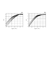
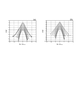
Following this procedure, the results are:
- Up to experimental errors, the functions $H(p)$ do not depend on the measurement location nor on the flow regime. The values ($H(p)=0.42,0.70,1.27,1.51,1.73\;{\rm for}\;p=1,2,4,5,6$) are those reported in HIT in numerous experiments [2, 21].
- The functions $n(\tau)$ do depend on the measurement location and flow regime. They are shown in figure 5 (the curves are normalized so that $n=0$ at integral time delays). We do not discuss hereafter the functional form of the $n(\tau)$ curves but the relative behaviour of the curves in each regime, when $r$ is varied. In (GR) one observes that in the outer region a larger range of scales is covered with a given number of cascade steps $n$ than in the vicinity of the vortex core. The slopes $dn(\tau)/d\tau$ increase as $r$ decreases, meaning that increasing number of steps are needed to cascade between any two given scales. Again, this is consistent with the idea that rotation prevents the 3D cascade and with our previous observation that it reduces the energy transfer to smaller scales. An inverse effect is observed in the (DR) regime: as measurements are performed closer to the rotation axis, $n(\tau)$ increases and is less steep, meaning that a wider range of scales is reached in a given number of cascade steps. This is consistent with a reduced slope of the velocity power spectra since such an efficient cascade provides an enhanced distribution of energy in the smaller scales.

6 Concluding remarks

Our foremost original observation is that some major caracteristics of HIT are retained in the vicinity of large scale coherent vortex structures: (i) the spectra develop an “inertial range” in the sense that power law scaling regions exist, (ii) the 3rd order structure functions yield consistent descriptions of the energy transfers and (iii) intermittency is always present and can be adequately described by a self-similar multiplicative cascade model. Second is that the structure and dynamics of the large scales influence the entire range of scales of motion. The combined study of power spectra, third order structure function and cascades parameters $H$ and $n$, give valuable informations that show that the turbulent cascade is reduced in the presence of global rotation and enhanced in the vicinity of very unstable vortex structures. Note that in the (GR) regime, eventhough the energy cascade is reversed and the spectra evolve towards a “$-3$” slope in the inertial zone, intermittency is observed: this a sharp difference with 2D turbulence [22] where no intermittency is detected although deviations from Gaussianity may be present [23].

***

It is a pleasure to acknowledge many useful discussions with B. Andreotti and B. Castaing.

***

References

- [1] Monin Yaglom, Statistical Fluid Mechanics, MIT Press, 1971
- [2] Frisch U., Turbulence, Cambridge U. Press, 1995
- [3] Malécot Y. et al., J. Fluid. Mech., preview (1999)
- [4] Chillà F., Pinton J.-F., Labbé R., Europhys. Lett., 35(4) 271 (1996)
- [5] Gaudin E. et al., Phys. Rev. E, 57(1) R9 (1998)
- [6] Camussi R., Guj G., J. FluidMech., 348 77 (1997)
- [7] Ruiz-Chavarria G., Leveque E., Ciliberto S., Baudet C., preprint, (1999)
- [8] Benzi R., Amati G., Casciola C.M., Toschi F., Piva R., preprint, (1999)
- [9] Tsinober A., Kit E., Dracos T., J. Fluid Mech., 242 169 (1992)
- [10] Andreotti B., Couder Y., Douady S., Europ J. Mech./B Fluids, 17 451 (1998)
- [11] Jimenez J., Wray A.A., Saffman P.G., Rogallo R.S., J. Fluid Mech., 255 65 (1993)
- [12] Malecot Y., PhD Thesis, Universtité Grenoble I, (1998)
- [13] Pinton J.-F., Chillà F., Mordant N., Eur. J. Phys. B/Fluids, 17 535 (1998)
- [14] Melander M.V., Hussain F., Phys. Rev. E, 48 2669 (1993)
- [15] Hossain M., Phys. Fluids, 6(3) 1077 (1994)
- [16] Labbé R., Pinton J.-F., Fauve S., J. Phys. II France, 6 1099 (1996)
- [17] Castaing B., Gagne Y., Hopfinger E., Physica D, 46 177 (1990)
- [18] Pinton J.-F., Plaza F., Danaila L., Le Gal P., Anselmet F., Physica D, 122 187 (1998)
- [19] Castaing B., Dubrulle B., J. Phys. II (France), 5(7) 895 (1995)
- [20] Benzi R., et al., Phys. Rev. E,, 48 R29 (1993)
- [21] Arneodo A. et al., Europhys. Lett., 34 411 (1996)
- [22] Paret J., Tabeling P., Phys. Fluids, 10 3126 (1998)
- [23] Boffeta G., Celani A., Vergassola M., chao-dyn/9906016,