Transition to Turbulence in
Coupled Maps on Hierarchical Lattices

Abstract

General hierarchical lattices of coupled maps are considered as dynamical systems. These models may describe many processes occurring in heterogeneous media with tree-like structures. The transition to turbulence via spatiotemporal intermittency is investigated for these geometries. Critical exponents associated to the onset of turbulence are calculated as functions of the parameters of the systems. No evidence of nontrivial collective behavior is observed in the global quantity used to characterize the spatiotemporal dynamics.

I Introduction.

Coupled map lattices are spatiotemporal dynamical systems comprised of an interacting array of discrete-time maps. Coupled map lattices have provided fruitful models for the study of many spatiotemporal processes in a variety of contexts Survey . In most of these studies, the dynamical processes have been assumed to take place on uniform Euclidean spaces. However; because of their discrete spatial nature, coupled map lattice systems seem especially appropriate for investigating physical phenomena occurring in heterogeneous media. In this respect, there are some recent models of coupled maps defined on fractal lattices Us1 ; Us2 , and also an investigation of coupled maps on a Cayley tree Gade .

In this article we consider coupled maps defined on generalized hierarchical lattices, or multi-branching trees, as dynamical systems. Examples of phenomena where hierarchical structures appear include DLA clusters, capillarity, chemical reactions in porous media Kopel , turbulence Sree , ecological systems Hogg , interstellar cloud complexes Scalo , etc. Hierarchical structures have also been studied in neural nets, because of their exponentially large storage capacity Admit . Although many hierarchical structures found in nature have random ramifications, here we study the case of simple, deterministic tree-like arrays. This allows to focus on the changes induced in spatiotemporal processes as a result of the hierarchical structure of the interactions in the system.

In Sec. II, coupled map lattice models for the treatment of generalized hierarchical lattices are presented. As an application, in Sec. III we study the phenomenon of spatiotemporal intermittency as a mechanism for the transition to turbulence in coupled maps on hierarchical lattices. The model is based on the one introduced earlier by Chaté and Manneville for regular Euclidean lattices in one and two dimensions Chate1 , and which captures the essential features of the transition to turbulence in extended systems. A discussion is given in Sec. IV.

II Coupled maps on hierarchical lattices.

Generalized trees constitute a class of hierarchical lattices which can be generated for any constant ramification number $k$. At the initial level (which we call level $0$), there is one cell which splits into $k$ branches connecting $k$ daughters cells, which constitute the level of construction $1$. Each cell then splits into $k$ daughters, producing $k^{2}$ sites at level $2$. This construction continues until some level $n$. There are $k^{m}$ cells at the level of construction $m$; $m=0,1\ldots,n$. Thus, each cell in the lattice has one parent and $k$ daughters, except for the level $0$ cell, which has no parent, and for boundary cells at level $n$, which have no daughters. The number of cells lying on the boundary is $k^{n}$.

Each cell in a tree constructed until level $n$ can be identified by an index $i=1,2,\ldots,N$, where $N$ is the total number of cells on the tree, or the system size, given by $N=(k^{n+1}-1)/(k-1)$.

A cell denoted by the index $i$ at a level $m$ is coupled only to neighbor cells belonging to adjacent levels on the lattice, i.e., to its parent and to its daughters, which we indicate by indexes $i_{p}$ and $i_{d}$, respectively. We do not consider interactions between cells belonging to the same level. Thus, a discrete diffusive coupling can be defined according to the following scheme. If $i=0$, then the cell is at the level $0$ of the network and it is coupled to its $k$ daughters, which have the indices $i=1,2\ldots,k$. Cells with $i>0$ are coupled to cells with indices $i_{p}$ and $i_{d}$, such as

$$i_{p}=\mbox{int}\left(\frac{i-1}{k}\right),$$ (1)

where the function int means integral part, and

$$i_{d}=(i\times k)+j;\quad j=1,2,\ldots,k;\quad\mbox{if}\;\;i<(N-k^{n}),$$ (2)

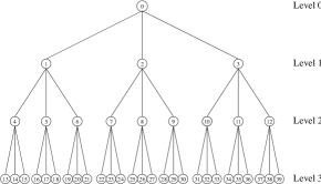
and $i_{d}$ is not defined for boundary cells, which have $i\geq(N-k^{n})$. The level $0$ cell has $k$ neighbors, intermediate cells have $k+1$ neighbors, and boundary cells for which $i>(N-k^{n})$ possess only one neighbor. As an illustration, Fig. (1) shows a hierarchical tree with ramification number $k=3$ and construction level $n=3$. The lattice size is $N=40$. The indices on each cell are indicated. In this example, the cell labeled by $i=11$ belongs to level $n=2$; its parent has index $i_{p}=3$, and its daughters are labeled by $i_{d}=34,35$, and $36$, respectively.

Figure 1: Hierarchical lattice with ramification $k=3$ and level of construction $n=3$, showing the indices on the cells.

The state of each site on the lattice can be assigned a continuous variable $x$, which evolves according to a deterministic rule depending on its own value and the values of its connecting neighbors. The equations describing the dynamics of a diffusively coupled map hierarchical lattice at level of construction $n$ can be written as

(a) level $0$ cell:

$$x_{t+1}(0)=(1-k\gamma)f(x_{t}(0))+\gamma\sum_{j\in i_{d}}f\left(x_{t}(j)\right);$$ (3)

(b) for $i<(N-k^{n})$,

$$\begin{array}[]{ll}x_{t+1}(i)=&\left[1-(k+1)\gamma\right]f(x_{t}(i))+\cr&\gamma f\left(x_{t}(i_{p})\right)+\gamma\sum_{j\in i_{d}}f\left(x_{t}(j)\right);\end{array}$$ (4)

(c) and for boundary cells with $i\geq(N-k^{n})$,

$$x_{t+1}(i)=f\left(x_{t}(i)\right)+\gamma f\left(x_{t}(i_{p})\right);$$ (5)

where $x_{t}(i)$ gives the state of the cell $i$ at discrete time $t$; $i_{p}$ and $i_{d}$ label the $N$ cells on the lattice; $\gamma$ is a parameter measuring the coupling strength between neighboring sites, and $f(x)$ is a nonlinear function describing the local dynamics. The above coupled map lattice equations can be generalized to include nonuniform coupling and/or varying ramifications within the network. By providing appropriate local dynamics and couplings, different spatiotemporal phenomena can be studied on tree-like structures.

III An application: transition to turbulence.

Spatiotemporal intermittency in extended systems consists of a sustained regime where coherent and chaotic domains coexist and evolve in space and time. The transition to turbulence via spatiotemporal intermittency has been studied in coupled map lattices whose spatial supports are Euclidean Chate1 ; Kan ; Stassi and also in fractal lattices Us2 . A local map possessing the minimal requirements for observing spatiotemporal intermittency is Chate1

$$f(x)=\left\{\begin{array}[]{ll}\frac{r}{2}\left(1-\left|1-2x\right|\right),&\mbox{if $x\in[0,1]$}\\ x,&\mbox{if $x>1$},\end{array}\right.$$ (6)

with $r>2$. This map is chaotic for $f(x)$ in $[0,1]$. However, for $f(x)>1$ the iteration is locked on a fixed point. The local state can thus be seen as a continuum of stable “laminar” fixed points $(x>1)$ adjacent to a chaotic repeller or “turbulent” state $(x\in[0,1])$.

In regular dimensions, the turbulent state can propagate through the lattice in time for a large enough coupling, producing sustained regimes of spatiotemporal intermittency Chate1 . Here, we investigate the phenomenon of transition to turbulence in hierarchical lattices using the local map $f$ (Eq.(6)) in the coupled system described by Eqs. (3)-(5). The local parameter is fixed at the value $r=3$ in all the calculations. As observed for regular lattices, starting from random initial conditions and after some transient regime, our systems settle in a stationary statistical behavior. The transition to turbulence can be characterized through the average value of the instantaneous fraction of turbulent sites $F_{t}$, a quantity that serves as the order parameter Chate1 . We have calculated $\langle F\rangle$ as a function of the coupling parameter $\gamma$ for several hierarchical lattices from a time average of the instantaneous turbulent fraction $F_{t}$, as

$$\langle F\rangle={1\over T}\sum_{t=1}^{T}F_{t}.$$ (7)

About $10^{4}$ iterations were discarded before taking the time average in Eq. (7) and $T$ was typically taken at the value $10^{4}$. Fig. (2) shows $\langle F\rangle$ vs. $\gamma$ for hierarchical lattices with ramification numbers $k=2,3$ and $4$, and levels of construction $n=12,8$ and $7$, respectively. We have verified that increasing the averaging time $T$ or the lattice size $N$ does not have appreciable effects on our results. The standard deviations about each value of $\langle F\rangle$ are very small on the scale of Fig. (2). In fact, the fluctuations of $F_{t}$ become smaller for increasing ramification $k$ and/or for higher levels of construction. In comparison, high dimensional Euclidean lattices Chate3 , as well as fractal lattices Us2 and globally coupled maps CP , exhibit large oscillations in the time series of the instantaneous turbulent fraction $F_{t}$ for some parameter values. In those cases, the fluctuations about the mean values of the turbulent fraction do not decrease with increasing lattice size or averaging time, pointing to the presence of nontrivial collective behavior in the systems. In contrast, normal statistical properties are observed in hierarchical arrays of coupled maps, even in the cases when these lattices have the same numbers of local connections than the other arrays. Note that fractal lattices are also spatially nonuniform. However, the behavior of a statistical variable such as the turbulent fraction, is different for hierarchical lattices. Calculations of the mean field in Cayley trees using local logistic maps neither show evidence of nontrivial collective behavior Gade . Thus, the topology of the underlying geometry seems to have a relevant influence on the kind of behavior that may emerge in global quantities in spatiotemporal systems.

Figure 2: Mean turbulent fraction $\langle F\rangle$ as a function of the coupling $\gamma$ for different hierarchical lattices. Thick left curve, $k=2$, $n=12$; middle curve, $k=3$, $n=8$; thin right curve, $k=4$, $n=7$. The local parameter is fixed at $r=3$.

There exists a critical value of the coupling $\gamma_{c}$ for the onset of turbulence which becomes smaller for increasing ramification of the trees. The threshold for intermittency is achieved when the probability of reinjection into the unit interval is balanced by the probability of escape from this interval, which is constant for fixed $r$. The former is proportional to $\gamma$ and to the number of coupled neighbors, one of them at least being turbulent. Thus, $\gamma_{c}$ must decrease with increasing $k$, for fixed $r$. Fig. (3) shows $\gamma_{c}$ as a function of the ramification number $k$, verifying this assumption.

Figure 3: Critical coupling $\gamma_{c}$ as a function of the ramification $k$.

As for other lattices, the transition from a laminar regime to turbulence can be characterized by critical exponents like $\beta$ which scales the variation of the order parameter near the transition point: $\langle F\rangle\sim(\gamma-\gamma_{c})^{\beta}$. We numerically checked this relation. Our results are given in Fig. (4) for lattices with different ramification numbers, using a log-log plot.

Figure 4: Log-log plot of $\langle F\rangle$ vs $(\gamma-\gamma_{c})$ for hierarchical lattices: $k=2$ ($+$); $k=3$ ($\times$); $k=4$ ($\circ$).

Table (1) gives the critical exponents $\beta$ calculated from the slopes of Fig. (4) for different ramifications $k$, with their respective errors. The values of $\beta$ for these hierarchical lattices with different ramifications are of the order of that of a one-dimensional lattice, which is $\beta=0.250\pm 0.005$ Chate1 . Thus, the statistical properties of the transition to turbulence for hierarchical lattices are closer to that of a one-dimensional lattice in this scenario. It should also be noticed that the global dynamics of one-dimensional coupled map lattices neither display nontrivial collective behavior Chate4 .

$k$	$n$	$\beta$
$\ \quad 2\ \quad$	$\ \quad 13\ \quad$	$\ \quad 0.21\pm 0.01\ \quad$
$3$	$8$	$0.22\pm 0.02$
$4$	$7$	$0.25\pm 0.03$
$5$	$7$	$0.28\pm 0.02$

Table 1: Critical exponents $\beta$ for hierarchical lattices with different ramifications $k$. The corresponding levels of construction $n$ are also indicated.

IV Discussion.

We have introduced coupled map lattice systems with hierarchical couplings. These models are especially suited for investigating spatiotemporal phenomena occurring in heterogeneous media with an underlying tree-like geometry, and they may also represent the hierarchical interactions taking place in some organized systems.

Although we employed the simple Chaté-Manneville map for illustrating the transition to turbulence on hierarchical lattices, more sophisticated coupled map models may prove useful in the study of fully developed turbulence in fluids, where dissipation of energy occurs in hierarchical cascades from larger to smaller structures Sree .

In hierarchical lattices, as defined in Sec. II, there exists a unique path connecting any two given elements on the network. This same topological property occurs in a one-dimensional lattice with open ends. The similarity in the scaling behavior at the transition to turbulence between hierarchical lattices of different ramifications and a one-dimensional lattice suggests that topological properties of the underlying lattice are relevant in the global behavior of spatiotemporal systems.

In addition, the global quantity Eq. (7) follows a normal statistical behavior in hierarchical lattices, while nontrivial collective oscillations arise in other geometries. Hierarchical lattices have different topological properties than those of regular higher dimensional Euclidean arrays or fractal lattices which have previously been considered as coupled map systems. No closed loops exist in hierarchical lattices, and the number of local connections is not uniform since an appreciable fraction of cells possessing only one neighbor lie on the boundary. As it has been suggested Us2 ; Chate4 ; Mc , the topology of the lattice seems to play a more important role on the emergence of collective behaviors than the number of local connections or the dimensionality of the space. The failure to observe collective behavior in our models also points to this conclusion. Future work on hierarchical and other nonuniform lattices may contribute to answer this and other remaining questions on the collective dynamics of chaotic extended systems.

References

- (1) Theory and Applications of Coupled Map Lattices, Chaos 2, No. 3, edited by K. Kaneko, Wiley, N. Y., (1993).
- (2) M. G. Cosenza and R. Kapral, Phys. Rev. A 46, 1850 (1992); Chaos 2, 329 (1992).
- (3) M. G. Cosenza and R. Kapral, Chaos 4, 99 (1994).
- (4) P. M. Gade, H. Cerdeira, and R. Ramaswamy, Phys. Rev. E 52, 2478 (1995).
- (5) The Fractal Approach to Heterogeneous Chemistry, edited by D. Avnir, Wiley, New York, 1989.
- (6) C. Meneveau and K. R. Sreenivasan, Phys. Rev. Lett. 59, 1424 (1987).
- (7) T. Hogg, B. A Huberman and J. McGlade, Proc. R. Soc. London B 237, 43 (1989).
- (8) P. Houlahan and J. Scalo, Ap. J. 393, 172 (1992).
- (9) D. Admit, Modeling Brain Function: The World of Attractor Neural Nets, Cambridge U. Press, Cambridge, 1989.
- (10) H. Chaté and P. Manneville, Physica D 32, 409 (1988); Europhys. Lett. 6, 591 (1988).
- (11) K. Kaneko, Prog. Theor. Phys. 74, 1033 (1985).
- (12) D. Stassinopoulos and P. Alstrøm, Phys. Rev. A 45, 675 (1992).
- (13) H. Chaté and P. Manneville, in New Trends in Nonlinear Dynamics and Pattern Forming Phenomena, edited by P. Coullet and P. Heurre, Plenum, New York (1989).
- (14) M. G. Cosenza and A. Parravano, Phys. Rev. E 53, 6032 (1998).
- (15) H. Chaté and P. Manneville, Prog. Theor. Phys. 87, 1 (1992); Chaos 2, 307 (1992).
- (16) M. G. Cosenza, Physica A 257, 357 (1998).