The effects of large scales on the inertial range in high-Reynolds-number turbulence

Abstract

The effects of removing large scales external to the inertial range on the properties of scales within the inertial range are studied in a high-Reynolds-number turbulent flow. Structure functions of both even and odd orders are strongly affected across the entire inertial range, but odd-order moments are affected to a greater degree. In particular, the skewness of velocity increments shows a significant reduction whereas the flatness changes comparatively little. The reduction in skewness is counterbalanced essentially by the interaction between the small-scale energy and the large-scale rate of strain. The implications of these results for the conventional cascade picture are examined briefly.

PACS Numbers: 47.27.Ak, 47.27.Jv

1 Introduction

The Kármán-Howarth equation¹ is an exact dynamical equation for the second-order correlation function in isotropic turbulence. The equation is easily expressed in terms of the longitudinal structure function $S_{2}(r,t)$, where $S_{2}\equiv\langle\Delta u_{r}^{2}\rangle\equiv\langle[u(x+r)-u(x)]^{2}\rangle$, $u(x)$ is the turbulent velocity component in the direction $x$, and $r$ is the separation distance in that same direction. Assuming that the time variation of $S_{2}$ is slow, Kolmogorov² reduced the Kármán-Howarth equation to an equation for the third-order structure function. This equation, given by

$$S_{3}(r)\equiv\langle[u(x+r)-u(x)]^{3}\rangle=-\frac{4}{5}\langle\varepsilon\rangle r+6\nu\frac{\partial S_{2}(r)}{\partial r},$$ (1)

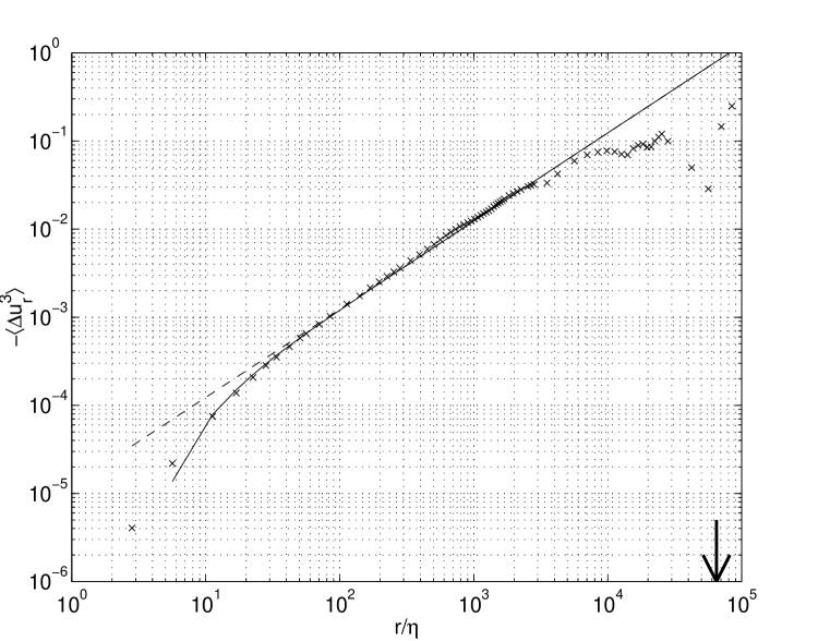
Figure 1: The (negative value of the) third-order structure function, $S_{3}$, plotted against the separation distance, $r$, normalized by the Kolmogorov scale $\eta$. The measured data are compared with Eq. (1), full line. The agreement is quite good up to $r=H/20$. The largest disagreement, seen at the very small scales, is due to the difficulty of resolving those scales well. The dashed line, which differs from Eq. (1) only below $r/\eta$ of about 50, is Eq. (2). The data are for the atmospheric surface layer at the height $H=35$ m above the ground, and all averages are over time; details of measurements are given in Sec. II. Here, $H$ is treated as the representative large scale, and marked by an arrow on the abscissae.

has been rederived under less restrictive circumstances^3,4, and works well in shear flows as long as $r$ is much smaller than a characteristic large scale, $L$. Here $\langle\varepsilon\rangle$ is the average value of the energy dissipation rate. Figure 1 is a typical comparison between the measured third-order structure function and the right hand side of Eq. (1). In particular, there is a range of scales over which the viscous term is negligibly small, and we have

$$S_{3}(r)=-\frac{4}{5}\langle\varepsilon\rangle r.$$ (2)

Indeed, it is conventional to define the inertial range as the range of scales for which this equation is valid.

The usual interpretation of Eq. (2) is that, on the average, it prescribes a unidirectional down-scale energy flux.^5,3 It is consequently thought that the statistical physics appropriate to the inertial range has a strongly non-equilibrium character.⁶ On the other hand, consider the following argument. If the inertial range dynamics is not influenced by viscosity (as apparent in the previous paragraph), it is reasonable to suppose that the dynamics there is governed essentially by the Euler equations. The Euler equations possess time-reversal symmetry, $t\rightarrow-t$, $\bf u\rightarrow\bf-u$ (t = time, $\bf u$ = vector velocity), which could therefore be interpreted to mean that the energy flow in the inertial range is essentially as much up-scale as down-scale. The proper meaning of Eq. (2) would then be that the energy flux it prescribes is a small difference between equally large energy flows in the up-scale and down-scale directions. The finiteness of $S_{3}$ may then mean that there exists no more than a “small leakage” between two opposing and equally strong fluxes.⁷ If this is true, the situation calls for a simpler type of statistical physics.

Prompted by such qualitative considerations, we studied, some nine years ago,⁸ the source of energy flux in the Kolmogorov equation. A result of particular interest is the experimental finding that $S_{3}$ became small when large scales in the fluctuating velocity were filtered out. This result was thought to imply that the Kolmogorov result, Eq. (2), was more a reflection on the source of the energy flux (large scales) than a statement about unidirectional cascades. We present here an up-date of the experimental part of that (unpublished) study. We use velocity signals acquired in a very high-Reynolds-number atmospheric surface layer, described below, to analyse the effect of removing large scales on the statistics of $\Delta u_{r}$, in particular the effects on its third moment. The principal conclusion is that, while the removal of large scales affects both even-order and odd-order moments of velocity increments in the inertial range, the odd moments are much more vulnerable. The results are interpreted briefly in the light of the issues raised above, though it is fair to warn the reader that we shall not be able to resolve the issue satisfactorily. Section II is a brief commentary of the experimental data, while Sec. III presents the basic experimental results. The chief conclusions are discussed in Sec. IV.

2 The data and the filter characteristics

The filtering experiments to be described below have been made for a number of flows such as a pipe flow (diameter Reynolds number $\approx$ 230,000), boundary layer turbulence (boundary layer thickness Reynolds number $\approx$ 20,000), atmospheric turbulence at a height of 6 m above the ground (Taylor microscale Reynolds number $R_{\lambda}\approx$ 2,000), and atmospheric turbulence at a height of 35 m above the ground ($R_{\lambda}\approx$ 10,000).⁹ The results are entirely consistent with each other, but are more revealing when the Reynolds number is high and the scale separation large, so we present data only for the last case. Tests were made on several sets of data, but the results are presented for brevity for only one.

The atmospheric data were acquired by a hot-wire probe mounted at a height of 35 m above the ground on the meteorological tower at the Brookhaven National Laboratory. The wind speed and direction were independently monitored by a vane anemometer mounted close to the tower. During data acquisition, the mean wind was essentially steady in both magnitude and direction. This was ensured, a posteriori, by using only those sets of data for which the averages computed over different segments of the measurement interval were steady. The conditions of measurement thus approached ‘controlled’ circumstances.

The hotwire, about 0.7 mm in length and 5 $\mu$m in diameter, was operated in a constant temperature mode. Its frequency response was compensated to be flat up to 20 kHz. The voltage from the anemometer was low-pass filtered and digitized. The low-pass cut-off was half the sampling frequency, $f_{s}$, which was set at 5,000 Hz. This frequency was high enough to include essentially all the finest-scale turbulent fluctuations in the flow. The voltage was constantly monitored on an oscilloscope to ensure that it did not exceed the digitizer limits. The voltage from the anemometer was converted to wind velocity through the standard calibration procedure, which included calibrating the hotwire just prior to mounting and checking it immediately after dismounting. Taylor’s frozen flow assumption was employed to convert the time variable into the spatial distance.

The following characteristics pertain to the present data: The mean wind speed $\overline{U}$ $\approx$ 7.6 ms^-1, root-mean-square fluctuation velocity $u^{\prime}\approx$ 1.36 ms^-1, the mean energy dissipation rate $\langle\varepsilon\rangle\approx 3\times 10^{-2}$ m²s^-3, the Kolmogorov scale $\eta\approx$ 0.57 mm, the Taylor microscale in the streamwise direction $\lambda\approx 11.4$ cm. The Taylor microscale Reynolds number $u^{\prime}\lambda/\nu\approx 10,340$. We use the height from the ground, $H$, as a measure of the large scale. If we assume that the classical boundary layer arguments are valid, a characteristic scale for the large-scale transport is of the order $0.4\times 35$ m, where 0.4 is the ‘accepted’ numerical value of the Kármán constant.

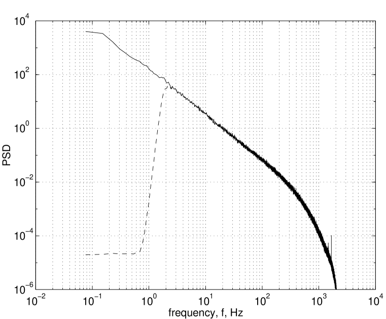
Figure 2: The full line is the power spectral density (PSD) of the longitudinal (streamwise) velocity fluctuation. The dashed line is the effect of a high-pass filter that is set to $f_{o}$ = 2 Hz. The filter is sharp and does not produce oscillations.

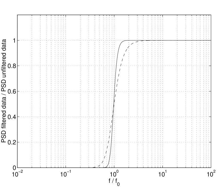
Figure 3: The ratio of the filtered to the unfiltered power spectral densities for the fourth and tenth order filters. We have experimented with both filters but used the tenth-order filter for the data presented in the rest of the text. For this filter, the filter effects essentially disappear for frequencies smaller than about $f_{o}/2$.

To obtain the filtered signal we used a Butterworth filter with excellent cut-off characteristics and no phase shift. The filtering operation was done by convolution in real space. The cut-off scale $r_{f}$ and the cut-off frequency $f_{o}$ are related by $r_{f}=U/f_{o}$. After filtering in the forward direction, the filtered sequence is reversed and run back through the filter. The resulting sequence has no phase distortion and double the filter order. We have used filters of order 4 and 10 (i.e., of order 2 and 5, respectively, but with two passes), mostly the latter. The filter characteristics are demonstrated in Figs. 2 to 4. (A different filtering scheme was employed in Ref. [8] and the nature of the results was identical.) Figure 2 shows the energy spectral density of streamwise velocity fluctuations. The Kolmogorov scaling of the spectral density for the unfiltered signal extends roughly over three decades of scales. The spectrum for the filtered signal, with high-pass setting at 2 Hz is also shown for the tenth-order filter. The attenuation in Fourier space exceeds 40 dB per octave. The ratio of the power spectral density of the filtered signal to that of the unfiltered signal is shown in Fig. 3 for fourth-order and tenth-order filters. For the latter, the filter effects vanish by within a factor of 2 of the cut-off setting.

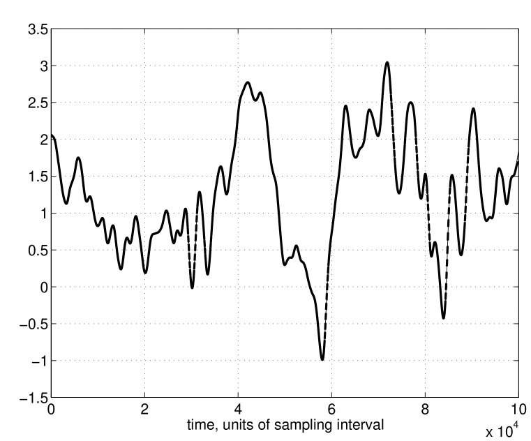
Figure 4: For a segment of the data, this figure compares the low-pass filtered part, $u^{<}$, with $f_{o}$ set at 2 Hz (full line), with $u_{*}^{<}\equiv u-u^{>}$ where $u^{>}$ is the high-pass filtered part obtained by an independent filtering operation, also performed with $f_{o}$ set to 2 Hz (heavy dashed line). The agreement between the two is excellent, as should be expected if the filtering operation produced no significant phase distortion.

The filter produces minimal phase distortion, as demonstrated below. Let $u$ be the unfiltered velocity, and $u^{>}$ and $u^{<}$ be the high-pass (small-scale) and low-pass (coarse-scale) parts of $u$, both obtained by independent filtering operations with the filter set at $f_{o}$ Hz. Define $u_{*}^{<}=u-u^{>}$. If the filter does not produce any phase distortion, we should find $u^{<}=u_{*}^{<}$. Figure 4 shows this is indeed so.

3 Experimental results

3.1 Probability density functions

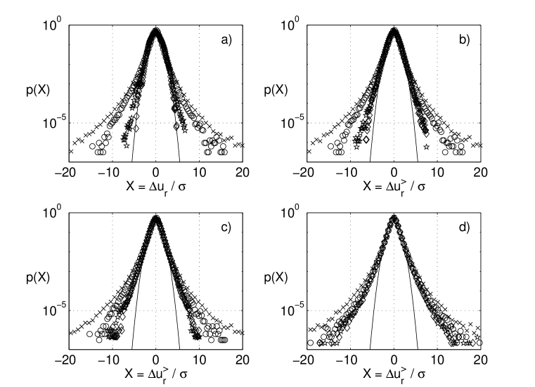
Figure 5: The effect of filtering on the probability density functions of $\Delta u_{r}$. In each case, the pdf is normalized by its own standard deviation, generically denoted by $\sigma$. The pdfs correspond to the following separation distances, $r$. $\times$: $r/H\approx 2.2\times 10^{-4}$, $r/\eta\approx 13$; $\circ$: $r/H\approx 3\times 10^{-3}$, $r/\eta\approx 186$; $\star$: $r/H\approx 0.3,~{}r/\eta\approx 18,670$; $\diamond$: $r/H\approx 3,~{}r/\eta\approx 1,86,700$. —, Gaussian. Figure (a) is for the unfiltered signal; (b) is for data high-pass filtered at $f_{o}=0.025$ Hz, $r_{f}/H\approx 9$, $r_{f}/\star\approx 120,000$; (c) $f_{o}$ = 2 Hz, $r_{f}/H\approx 0.11,~{}r_{f}/\eta\approx 1,500$; (d) $f_{o}$ = 25 Hz, $r_{f}/H\approx 8.8\times 10^{-3},~{}r_{f}/\eta\approx 116$.

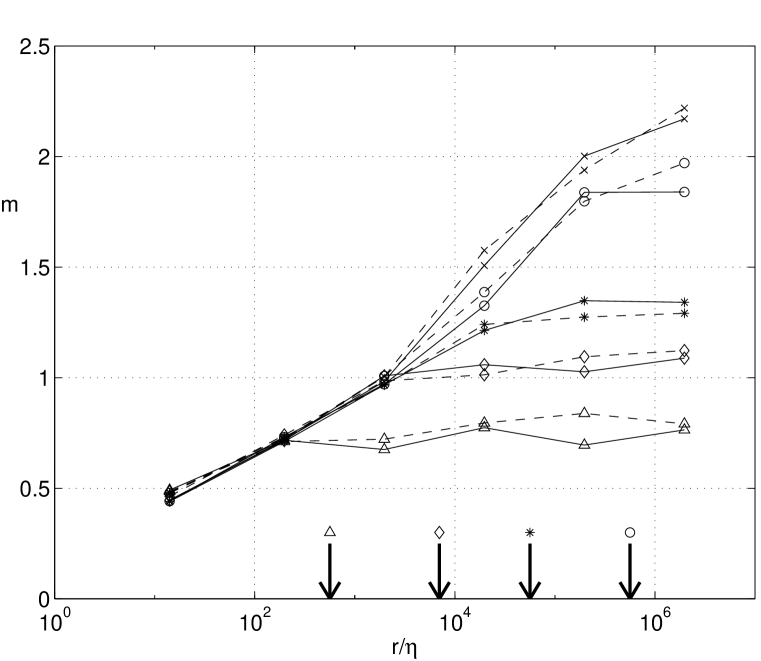
Figure 6: The stretching exponent, $m$, versus the separation distance for the unfiltered and filtered data sets. The values of $m$ are obtained by fitting empirically $p_{\Delta u_{r}}=p(0)exp[-c|\Delta u_{r}|^{m(r)}]$ over the entire range of $\Delta u_{r}$ except towards the tails where there is some scatter because of unconverged statistics. — is for the positive part of the pdf, and $-~{}-$ is for the negative part. $\times$, unfiltered; $\circ$, high-pass filtered at $f_{o}=0.025$ Hz ($r_{f}/H\approx 8.8$); $\ast$, $f_{o}$ 0.25 Hz ($r_{f}/H\approx 0.88$); $\diamond$, $f_{o}$ = 2 Hz ($r_{f}/H\approx 0.11$); $\triangle$, $f_{o}$ = 25 Hz ($r_{f}/H\approx 0.009$). Arrows mark the corresponding $r_{f}/\eta$ values. For the unfiltered data, the pdf tends essentially to a Gaussian ($m\approx 2$)—actually slightly sub-Gaussian because $m>2$; fo r the filtered cases, the asymptotic shapes depend on the respective cut-off scales.

It is known^10-12 that the probability density function (pdf) of the velocity increment, $\Delta u_{r}$, continually changes its character as the separation distance $r$ is varied: it is roughly square-root exponential for $r$ in the dissipative range and Gaussian when $r$ is comparable to the large scale. The pdfs are shown in Fig. 5 (a). Figures 5 (b), (c) and (d) show similar data for high-pass filtered signals, each for a different filter setting. The spatial cut-off scale $r_{f}$ is given in the caption. The removal of the large scales changes the pdfs in two respects: (1) the shape is affected significantly for separation distances $r$ smaller than the smallest scale removed by filtering, the latter being of the order $r_{f}$; (2) the asymptotic form of the pdf, for $r>r_{f}$, does not differ much from that at $r=r_{f}$, and is far from Gaussian. These effects can be quantified by fitting a stretched exponential, $p_{\Delta u_{r}}=p(0)exp[-c|\Delta u_{r}|^{m(r)}]$, to the pdfs of filtered signals, and comparing the stretching exponent $m(r)$ for various filter settings. This is done in Fig. 6. The exponent $m$ is slightly different for positive and negative sides of the distribution (shown by full and dashed lines, respectively), but these differences do not mask the major effect: the exponent is noticeably smaller for filtered signals than for the unfiltered signal, and the effect occurs at scales significantly smaller than the smallest filtered scale.

3.2 The third-order structure function

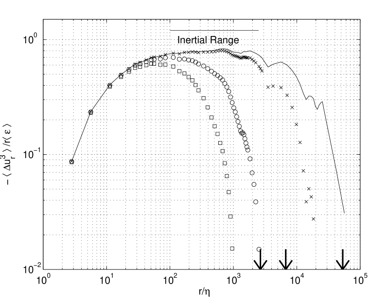
Figure 7: The Kolmogorov function $\langle\Delta u_{r}^{3}\rangle/r\langle\varepsilon\rangle$ plotted for unfiltered (—) and high-pass filtered traces ($\times$, $f_{o}$ = 0.25 Hz, $r_{f}/H\approx 0.88$; $\circ$, $f_{o}$ = 2 Hz, $r_{f}/H\approx 0.11$; $\Box$, $f_{o}$ = 5 Hz, $r_{f}/H\approx 0.044$). The normalizing scales $\eta$ and $\langle\varepsilon\rangle$ are for the unfiltered signal, but the filtering does not change them to any significant extent. The horizontal line extending between $r/\eta$ of 100 and 2500 is the estimated inertial range. In this figure and others to follow, the cut-off scale $r_{f}$ is shown by an arrow on the abscissae. The removal of large scales affects scales that are typically two decades smaller than $r_{f}$.

Figure 7 is a summary of the effects of the filtering operation on the third-order structure function. The ordinate is normalized by $r\langle\varepsilon\rangle$, and the separation distance is normalized by the Kolmogorov scale $\eta$ for the unfiltered data. First, a remark is in order on the function $K\equiv\langle\Delta u_{r}^{3}\rangle/r\langle\varepsilon\rangle$ for the unfiltered data: the inertial range, defined as the region where $K$ is flat and equal to 4/5, ranges roughly between $100\eta$ and $2500\eta$. (Note that the spectral density shown in Fig. 1 appears to possess a larger scaling range, but it is more prudent to base this estimate on the basis of Eq. (2).)

The high-pass filtered data are obtained by removing all scales above 30 m (frquencies below about 0.25 Hz), 3.8 m ($\sim$ 2 Hz) and 1.5 m ($\sim$ 5 Hz). The arrows mark the values of $r_{f}/\eta$. For the 3.8 m case, for example, $\langle\Delta u_{r}^{3}\rangle$ is smaller by an order of magnitude for $r/r_{f}=0.5$, by a factor 2 for $r/r_{f}=10$, and by about 10% for $r/r_{f}=100$. Inferring roughly from Fig. 2 that the artifacts of the filtering operation do not extend to scales smaller than about $r_{f}/2$, it is clear that the removal of large scales beyond the upper edge of the inertial range ($\sim$ 1.7 m) has a strong effect throughout the inertial range. However, the dissipation scales are not affected significantly, so $\langle\varepsilon\rangle$ and $\eta$ remain essentially the same as for the unfiltered data; we have therefore simply used the unfiltered values for normalization. The dissipation scales just begin to feel the effect of filtering for $r_{f}$ = 1.5 m, but this cut-off begins to encroach directly on the inertial range itself. For most of the results below, we shall use $r_{f}$ = 3.8 m ($\sim f_{o}$ = 2 Hz), unless stated otherwise.

A naive interpretation of Fig. 2 is that the large scales contribute significantly to $\langle\Delta u_{r}^{3}\rangle$ in the inertial range. A closer look demands a more complex interpretation. By splitting, as before, the velocity signal $u$ into the fine-scale (high-frequency) and coarse-scale (low-frequency) velocity components $u^{>}$ and $u^{<}$, separated by the cut-off scale $r_{f}$ or the cut-off frequency $f_{o}$, and noting that $u=u^{>}+u^{<}$ and $\Delta u_{r}=\Delta u_{r}^{>}+\Delta u_{r}^{<}$, the third-order structure function can be written as

$$\langle\Delta u_{r}^{3}\rangle=\langle(\Delta u_{r}^{>})^{3}\rangle+3\langle(\Delta u_{r}^{>})^{2}\Delta u_{r}^{<}\rangle+3\langle(\Delta u_{r}^{<})^{2}\Delta u_{r}^{>}\rangle+\langle(\Delta u_{r}^{<})^{3}\rangle.$$ (3)

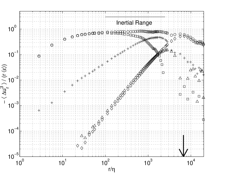
Figure 8: The result of decomposing the third-order structure function $\langle\Delta u_{r}^{3}\rangle$ in terms of $\Delta u_{r}^{<}$ and $\Delta u_{r}^{>}$; $f_{o}=2$ Hz, $r_{f}/H\approx$ 0.11. $\circ$, $\langle\Delta u_{r}^{3}\rangle/r\langle\varepsilon\rangle$; $\Box$, $\langle(\Delta u_{r}^{>})^{3}\rangle/r\langle\varepsilon\rangle$; $+$, 3$\langle(\Delta u_{r}^{>})^{2}\Delta u_{r}^{<}\rangle/r\langle\varepsilon\rangle$; $\triangle$, 3$\langle(\Delta u_{r}^{<})^{2}\Delta u_{r}^{>}\rangle/r\langle\varepsilon\rangle$; $\diamond$, $\langle(\Delta u_{r}^{<})^{3}\rangle/r\langle\varepsilon\rangle$. In the upper part of the inertial range, the most dominant term is $3\langle(\Delta u_{r}^{>})^{2}\Delta u_{r}^{<}\ ra$.

In the above equation, it is not hard to argue that $\langle(\Delta u_{r}^{<})^{3}\rangle$ and 3$\langle(\Delta u_{r}^{<})^{2}\Delta u_{r}^{>}\rangle$ should both be small for very small $r$, and that the term $\langle(\Delta u_{r}^{>})^{3}\rangle$ should approach $\langle\Delta u_{r}^{3}\rangle$ itself as $r\rightarrow 0$. For intermediate values of $r$, it is not easy to estimate the correct orders of magnitude of these terms. Experimental data (see Fig. 8) show that the largest term is $\langle(\Delta u_{r}^{>})^{3}\rangle$ in the lower part of the inertial range and 3$\langle(\Delta u_{r}^{>})^{2}\Delta u_{r}^{<}\rangle$ in the upper part, until they are both overtaken, as $r\rightarrow r_{f}$, by the exclusively large-scale part $\langle(\Delta u_{r}^{<})^{3}\rangle$.

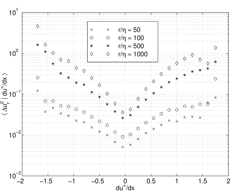
Figure 9: The conditional expectation of the unfiltered variance $(\Delta u_{r})^{2}$ conditioned on the rate of strain of the largest scale retained in the filtering operation, $d\Delta u_{r}^{<}/dx$; $f_{o}=2$ Hz, $r_{f}/\eta\approx$ 7,000. The various symbols correspond to different scale separations $r$, as noted in the inset.

The dominance of the term 3$\langle(\Delta u_{r}^{>})^{2}\Delta u_{r}^{<}\rangle$ suggests that a significant part of the third-order structure function comes from the straining of the small-scale kinetic energy, $(\Delta u_{r}^{>})^{2}$, by the large-scale feature $\Delta u_{r}^{<}$. This suggests the existence of a coupling between scales that are significantly separated. The effect is illustrated in a different manner in Fig. 9 where the second order moment of $\Delta u_{r}$, conditioned on the velocity gradient of the cut-off scale, $du_{r}^{<}/dr_{f}$, is plotted against the latter quantity; the conditioning variable is the gradient of the largest scale rejected by the filtering operation. The variance may be expected to be independent of the conditioning variable if the energy transfer across scales were purely a local phenomenon—in contrast to the measured effect.

3.3 Odd versus even moments

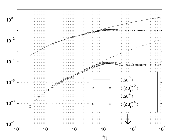
Figure 10: Second and fourth order structure functions for the unfiltered (lines) and filtered data (symbols). — and $\times$ are for the second-order; $-~{}-$ and $\circ$ are for the fourth-order; $f_{o}=2$ Hz, $r_{f}/\eta\approx$ 7,000.

The second and fourth order structure functions for the unfiltered and filtered data are shown in Fig. 10. Filtering has some effects on even-order moments as well; the larger the moment order, the larger this influence. However, these effects are much weaker than that for the third-order moment (and for other odd-order moments as well, though not shown here). Two specific statements can be made. First, for the second-order structure function, the filter is felt only up to scales that are at best an order of magnitude smaller than $r_{f}$, but the effect on the third-order extends to scales that are smaller by one further order of magnitude. Second, the effects on the third-order are larger than those on the next-higher even moment, namely the fourth.

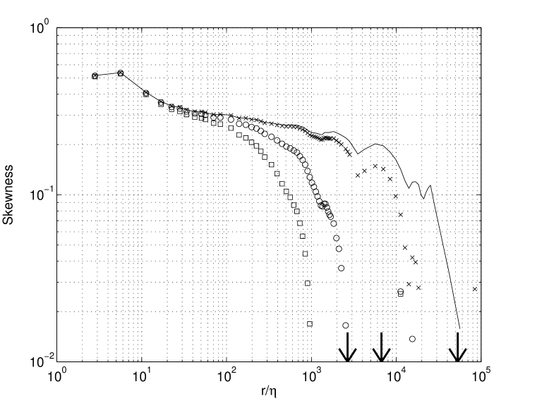
Figure 11: The skewness of velocity increments for the unfiltered (—) and filtered signals ($\times,f_{o}=0.25$ Hz, $r_{f}/H\approx 0.88$; $\circ,f_{o}=2$ Hz, $r_{f}/H\approx$ 0.11; $\Box$, $f_{o}=5$ Hz, $r_{f}/H\approx$ 0.044). The filter settings are shown by arrows.

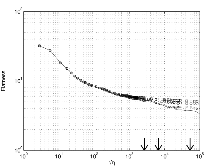
Figure 12: The flatness factor of velocity increments for the unfiltered (—) and filtered signals ($\times,f_{o}=0.25$ Hz, $r_{f}/H\approx 0.88$; $\circ,f_{o}=2$ Hz, $r_{f}/H\approx$ 0.11; $\Box$, $f_{o}=5$ Hz, $r_{f}/H\approx$ 0.044). The filter settings are shown by arrows.

A better appreciation for differences between odd and even moments can be gained by examining normalized moments. Figure 11 shows the skewness of the velocity increment for the three filter settings used above, as well as for the unfiltered data. A comment first on the unfiltered signal itself: the fact that the skewness of the unfiltered signal is not constant in the inertial range shows that the $r$-dependence of $\langle\Delta u_{r}^{2}\rangle$ has a power-law exponent that is higher than 2/3. While a rough estimate of this “anomalous correction” for second-order structure function can be obtained from this graph, it has been argued elsewhere⁹ that a proper estimate needs greater care. This is not our main point, so we shall make no further reference to it here. Note that the effect of removing scales above 30 m (below 0.25 Hz) already penetrates the inertial range; removing scales above 3.8 m (below 2 Hz) and 1.5 m (5 Hz) significantly reduces the skewness of scales everywhere in the inertial range. For instance, the skewness for the 2 Hz case is reduced by a factor of 2 for scales one order of magnitude smaller than $r_{f}$. On the other hand, the flatness of $\Delta u_{r}$ shows hardly any effect for scales smaller than $r_{f}/2$ (Fig. 12).

4 Discussion and conclusion

A principal conclusion of this work is that the removal of large scales significantly affects the statistics well into the inertial range. In terms of the normalized moments of velocity increments, the skewness—as are other odd moments—is affected much more strongly than the flatness—or other even moments. Indeed, if the large scales can be thought of as related, loosely, to the “size of the system”, it appears that the system-size effects are felt more strongly on odd moments than on even moments of velocity increments.

It is worth asking if this effect is special to shear flows, because all the flows we have explored are shear flows. But we have some experience in assessing the shear effects⁹ on scaling, and this experience suggests that the present conclusion is not restricted. It would, however, be worth repeating these calculations for isotropic turbulence. We have not done so because all the isotropic data available to us—experimentally as well as by simulations—possess limited scale separation, which makes i t very difficult to extract meaningful results.

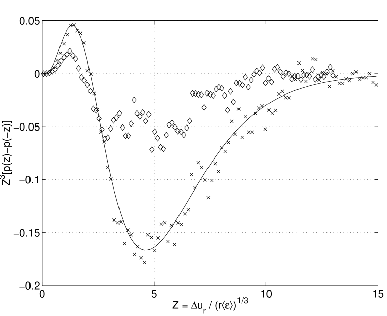
Figure 13: The integrand of $K\equiv\langle\Delta u_{r}\rangle^{3}/r\langle\varepsilon\rangle$, plotted against $\Delta u_{r}/(r\langle\varepsilon\rangle)^{1/3}$. The crosses are for the unfiltered signal, $r/\eta=1000$, and — represents a smooth line through them. The corresponding quantity for the filtered data, with $f_{o}=2$ Hz, $r_{f}/\eta\approx$ 7000, are shown by diamonds. The effect of the filter is drastic at all scales. The relatively large scatter in the data is the result of taking the difference between two nearly equal quantities.

It must be emphasized that the present results do not suggest that the skewness of the velocity increment resides in the large $r$. Rather, what they suggest is that this asymmetry of the pdf is related to the straining of the energy in the inertial range by large scales. The asymmetry is the subject of another study in its own right,¹³ but it should be pointed out that it is associated with all magnitudes of $\Delta u_{r}$. To see this, consider the difference between the two sides of the pdf of $z\equiv\Delta u_{r}/(r\langle\varepsilon\rangle)^{1/3}$. The quantity $z^{3}\times[p(z)-p(-z)]$, when integrated over $0<z<\infty$, yields the function, $K\equiv\langle\Delta u_{r}^{3}\rangle/r\langle\varepsilon\rangle$. This integrand $z^{3}\times[p(z)-p(-z)]$ is plotted against $z$ in Fig. 13. The figure shows, for these specific conditions, that most of the contribution to $K$ comes largely from $z$ lying between about 2 and 10. The small values of $z$ lying between 0 and 2 make the opposite contribution to $K$. The filtering operation essentially affects the integrand everywhere.

What do the present results imply for the energy cascade and the nature of non-equilibrium (or otherwise) prevailing in the inertial range? They show that there are significant nonlocal effects, and that the energy cascade, even as an average concept, is not driven entirely by local effects. While cascade models do have pedagogi cal value, they seem to miss this element. However, interpretations on the non-equilibrium nature of inertial-range dynamics are difficult because the information at hand is very limited. While it is unclear that the time reversal symmetry of the Euler equations guarantees the near-equality of fluxes in both directions (for instance, Euler equations can in principle produce energy flux by an inviscid mechanism¹⁴), it is equally unclear that Eq. (2) in itself demands a strong non-equilibrium situation in the inertial range.

As a contrast, it is worth remembering that the subtle manner in which irreversibility appears even in the simpler case of the kinetic theory of gases took a long time to unfold. One should therefore not feel too pessimistic about the inconclusiveness of the present situation.

Acknowledgements

The work arose initially from a collaboration with A.A. Migdal and V. Yakhot (theory) and with P. Kailasnath and L. Zubair (experiment). We express our sincere thanks to them. Since the time of writing the unpublished paper⁸ some nine years ago, we have discussed various aspects with A.J. Chorin, U. Frisch, R.H. Kraichnan, M. Nelkin, G. Parisi, I. Procaccia, and E.D. Siggia. We are grateful to them for their generous comments.

References

¹Kármán, T., von and L. Howarth, “On the statistical theory of isotropic turbulence”, Proc. Roy. Soc. A164, 192-215 (1938).

²A.N. Kolmogorov, “Energy dissipation in isotropic turbulence”, Dokl. Akad. Nauk. SSSR, 32, 19-21 (1941).

³U. Frisch, Turbulence: The Legacy of A.N. Kolmogorov, Cambridge University Press, Cambridge, 1995.

⁴R. Hill, “Applicability of Kolmogorov’s and Monin’s equations of turbulence”, J. Fluid Mech., 353, 67-81 (1997).

⁵A.S. Monin and A.M. Yaglom, “Statistical Fluid Mechanics: Mechanics of Turbulence”, vol. 2, M.I.T. Press, Cambridge, MA, 1975.

⁶R.H. Kraichnan and S. Chen, “Is there a statistical mechanics of turbulence?”, Physica D, 37, 160-172 (1989).

⁷A. Chorin, Vorticity and Turbulence, Springer-Verlag, New York, 1994.

⁸P. Kailasnath, A.A. Migdal, K.R. Sreenivasan, V. Yakhot and L. Zubair, “The 4/5-ths Kolmogorov law and the odd-order moments of velocity differences in Turbulence”, unpublished report, Yale University (1991), pp. 18.

⁹K.R. Sreenivasan and B. Dhruva, “Is there scaling in high-Reynolds-number turbulence?”, Prog. Theo. Phys. Suppl. 130, 103-120 (1998).

¹⁰B. Casting, Y. Gagne and E.J. Hopfinger, “Velocity probability density functions of high-Reynolds-number turbulence,” Physica, 46D, 177-200 (1990).

¹¹P. Kailasnath, K.R. Sreenivasan and G. Stolovitzky, “The probability density of velocity increments in turbulent flows”, Phys. Rev. Lett., 68, 2766-2780 (1992).

¹²P. Tabeling, G. Zocchi, F. Belin, J. Maurer and H. Williame, “Probability density functions, skewness and flatness in large Reynolds number turbulence”, Phys. Rev. E. 53, 1613-1621 (1996).

¹³ S.I. Vainshtein and K.R. Sreenivasan, “Kolmogorov’s 4/5-ths law and intermittency in turbulence”, Phys. Rev. Lett., 73, 3085-3089 (1994).

¹⁴L. Onsager, “Statistical hydrodynamics”, Nuovo Cimento, 6 (suppl.) 279-287 (1949).