Kinetic Theory of Dynamical Systems

Abstract

It is generally believed that the dynamics of simple fluids can be considered to be chaotic, at least to the extent that they can be modeled as classical systems of particles interacting with short range, repulsive forces. Here we give a brief introduction to those parts of chaos theory that are relevant for understanding some features of non-equilibrium processes in fluids. We introduce the notions of Lyapunov exponents, Kolmogorov-Sinai entropy and related quantities using some simple low-dimensional systems as “toy” models of the more complicated systems encountered in the study of fluids. We then show how familiar methods used in the kinetic theory of gases can be employed for explicit, analytical calculations of the largest Lyapunov exponent and KS entropy for dilute gases composed of hard spheres in $d$ dimensions. We conclude with a brief discussion of interesting, open problems.

1 Introduction

We consider here a classical many-particle system, a gas of hard spheres or of hard disks. Our principal concern will be to develop methods by means of which we can understand and calculate the properties of such gases as chaotic dynamical systems. It is, of course, well known that to describe the macroscopic, equilibrium properties of such gases, we can easily dispense with any knowledge of most of the dynamical properties of the particles of which the gas is composed. That is, one can use thermodynamics and equilibrium statistical mechanics, i.e. statistical thermodynamics, to describe the relevant equilibrium properties of the gas. All of the relevant microscopic properties of the system needed for statistical thermodynamics are contained in the partition sum, which is defined in terms of the Hamiltonian of the system. The partition function is based on a probability measure on phase space. The macroscopic properties are simply related to averages with respect to this measure, of certain microscopic expressions. Of course it is far from trivial to compute these averages for anything like a real physical system.

Our interest here, though, is to consider a gas as a mechanical system and to understand its behavior in time, rather than its equilibrium properties, and to try to make quantitative statements about the motion of the trajectories of the phase points that describe the gas, in the usual $2Nd$-dimensional phase-space, $\Gamma$-space, of the system, where $N$ is the number of particles, $d$ the number of the spatial dimensions of the system, $d=2$ or $3$, and the phase-space has $dN$ spatial coordinates and $dN$ momentum coordinates. We take the particles to be identical hard spheres or hard disks, each of mass $m$ and diameter $\sigma$. When we wish to describe the typical or average properties of the system, we must start with the specification of some useful probability measure, with respect to which averages can be defined. Any dynamical system, therefore, consists of: 1) a space $\Gamma$, 2) a measure $\mu(A)$, $A\subset\Gamma$, and 3) a transformation $S:\Gamma\rightarrow\Gamma$. We will see that the dynamical viewpoint can explain some features of macroscopic systems from their microscopic behavior. The explanations can be followed most easily in dynamical systems of very low dimensionality. However, even in simple low dimensional systems, dynamics may become so complicated that is is effectively impossible to follow the dynamics for long time, starting from a typical initial point, and we will be forced to consider typical behaviors using some appropriate probability measure. Our interest will be focused on chaotic systems which have the property that any uncertainty in the specification of the exact initial state of the system will grow exponentially in time, to the point where the future of a phase-space point can no longer be predicted to within a reasonable accuracy[1]. But we can still say something about probabilities.

It turns out that there is a close connection between the chaoticity of the system and issues like irreversibility on the macroscopic level and, for a gas of particles that interact with short-range forces, the validity of kinetic theory[2]. This connection will first be outlined in section 2, for low dimensional systems. A more extensive treatment can be found in Ref. [3]. In section 3 we return to a high dimensional system in the form of a hard sphere gas in equilibrium. At low densities we can use kinetic theory to calculate a measure of chaoticity called the largest Lyapunov exponent. In section 4 another chaotic characteristic of this system is calculated using kinetic theory: the Kolmogorov-Sinai entropy. In section 5 we make some concluding remarks and present some open questions.

2 Dynamical Systems

The standard approaches to the theory of non-equilibrium processes in fluids are based on three foundational pillars: (1) The identification of the macroscopic quantities of physical interest as averages of microscopic quantities over an appropriate ensemble of similarly prepared systems; (2) The use of the Liouville equation, either in its classical or in its quantum mechanical version, to compute the time evolution of the ensemble distribution function; and (3) The utilization of some kind of physically reasonable factorization assumption for the ensemble distribution function in order to transform the Liouville equation into a tractable equation whose solution can be used to make quantitative statements about the macroscopic quantities. Such a procedure is followed in the derivation of the Navier-Stokes fluid dynamic equations from the Liouville equation[4] for general fluids, and in the derivation of the Boltzmann transport equation, and its extensions to higher densities, from the Liouville equation for dilute and moderately dense gases. More phenomenological approaches to irreversible behavior in fluids often depend on explicit stochastic assumptions about the underlying dynamical processes taking place in the fluid[5].

While they are of the highest importance for the development of theories of irreversible processes in fluids, both of these approaches to irreversible behavior leave the answers to some fundamental questions obscure. In particular, these approaches offer only qualitative insights into the reasons for the validity of the stochastic assumptions imbedded in these various procedures – either through factorization assumptions, which in essence, are statements about correlations and probabilities – or through the replacement of the exact dynamics by a stochastic, Langevin-type, dynamics. Further, while the approaches outlined above do predict an approach to an equilibrium state, under the proper physical conditions, and do provide experimentally verifiable statements about the approach to equilibrium, they do not give a complete picture of why the system approaches an equilibrium state, based upon the underlying microscopic dynamics. The general arguments for the use of stochastic methods are based upon the randomness of the microscopic motions of the particles but are not much more specific than that. The picture that we have of the approach to equilibrium is generally based on the idea that the local averages of conserved mechanical quantities, such as mass, momentum, and energy, change very slowly in time compared to the local averages of nonconserved quantities. Thus the macroscopic behavior will be dominated by the slowest variables in the system, the local conserved quantities, and the equilibrium state will be achieved when these quantities have reached steady, homogeneous values. This picture, suggested by solutions of the Boltzmann equation, has led to important advances in the theory of fluids, among others, to mode-coupling theory. What is missing from it is a basic understanding of the necessary (or sufficient) properties of the intermolecular potential for the system to approach an equilibrium state, as well as an understanding of the properties of the trajectories of the system, and the evolution of measures in $\Gamma$-space, that are responsible for the approach to equilibrium states and, perhaps, under different boundary conditions, to more complicated, but interesting non-equilibrium steady states.

The application of ideas from dynamical systems theory to non-equilibrium statistical mechanics allows us to make some progress in resolving the issues described above. The application of ideas from chaos theory, in particular, enables us to make some quantitative statements about the type and degree of randomness of a dynamical system, even of large systems typically treated by statistical mechanics. It also allows us to describe equilibrium and non-equilibrium states of a system in terms of probability measures defined in $\Gamma$-space, and in terms of the time evolution of these measures. Moreover, there are interesting and unexpected connections between the macroscopic transport coefficients that describe the approach of a fluid to equilibrium, and microscopic quantities that describe the chaotic behavior of a fluid, considered as a large, dynamical system. In this section we will outline some of these rather new ideas, and illustrate their applications to statistical mechanics by seeing how they work for systems of low dimensions and then generalizing them, when possible, to higher dimensional systems. We begin with a very simple two-dimensional reversible system, the baker’s map, which exhibits many of the features we would like to see in more general, higher dimensional systems.

2.1 The baker’s map

The simplest example of a reversible system with chaotic dynamics is probably the baker’s map. Here we consider a two-dimensional phase space on a unit square. That is, $\Gamma=(x,y);0\leq x,y\leq 1$. The map, ${\bf B}$, operates only at discrete time steps, and moves points $(x,y)$ to ${\bf B}(x,y)=(x^{\prime},y^{\prime})$ given by

$${\bf B}\left(\begin{array}[]{c}x\\ y\end{array}\right)=\left(\begin{array}[]{c}x^{\prime}\\ y^{\prime}\end{array}\right) = \left(\begin{array}[]{c}2x\\ y/2\end{array}\right)\,\,\,\,\,{\mbox{for}}\,\,0\leq x<1/2;\,\,\,{\mbox{and}}$$ (7)

$$= \left(\begin{array}[]{c}2x-1\\ (y+1)/2\end{array}\right)\,\,\,\,\,{\mbox{for}}\,\,1/2\leq x<1.$$ (10)

This map is illustrated in Fig. 1. It is immediately clear that this map possesses an inverse, ${\bf B}^{-1}$, given by

$${\bf B}^{-1}\left(\begin{array}[]{c}x\\ y\end{array}\right) = \left(\begin{array}[]{c}x/2\\ 2y\end{array}\right)\,\,\,\,\,{\rm for}\,\,\,0\leq y<1/2\,\,\,{\mbox{and}}$$ (15)

$$= \left(\begin{array}[]{c}(x+1)/2\\ 2y-1\end{array}\right)\,\,\,\,\,{\mbox{for}}\,\,\,1/2\leq y<1.$$ (18)

The baker’s map is clearly area-preserving, and it is time-reversible in the sense that the transformation ${\bf T}:(x,y)\rightarrow(1-y,1-x)$ serves as a time reversal transformation for this map, such that ${\bf T}\circ{\bf B}\circ{\bf T}={\bf B}^{-1}$, and ${\bf T}\circ{\bf T}={\bf 1}$, where ${\bf 1}$ is the unit operator.

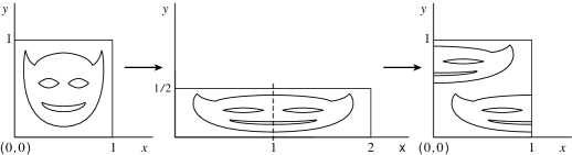
Figure 1: The baker’s transformation.

Now we regard the unit square as a “toy” phase-space. The dynamics of the baker’s map in this phase-space has the following properties: 1) Consider two infinitesimally separated points. Unless they have exactly the same $x$-coordinates, or the same $y$-coordinates, the images of these two points under several applications, called iterations, of the map ${\bf B}$ will cause the $x$-components to separate exponentially with the number of applications, with an exponent of $\lambda_{+}=\ln 2$, whereas the $y$-components will converge exponentially to a common value with an exponent of $\lambda_{-}=-\ln 2$. The exponents, $\lambda_{\pm}$, characterizing exponential separation or convergence of points in phase-space are called Lyapunov exponents. The directions in which the points converge exponentially, in this case just the $y$-direction, are called stable directions, and the directions in which they separate exponentially, in this case the $x$-direction, are called unstable directions. The fact that the Lyapunov exponents sum to zero is a simple consequence of the area preserving property of the baker’s map, as can easily be seen by considering the evolution, with successive iterations, of the small rectangle with corners at $(x,y),(x+\delta x,y),(x,y+\delta y),(x+\delta x,y+\delta y)$ under the baker map, ${\bf B}$. This rectangle has constant area, but grows exponentially long in the $x$-direction, and exponentially thin in the $y$-direction. Sooner or later it gets stretched and folded in such a way that on a coarse grained scale, the unit square is covered uniformly. We will describe this behavior on a coarse-grained scale, by saying that the distribution of points becomes weakly uniform. It is important to note that the projection of the small rectangle onto the $x$-axis will be uniform in a time, $n_{u}$ on the order of

$$n_{u}\sim\frac{-\ln\delta x}{\lambda_{+}},$$ (19)

where $\lambda_{+}=\ln 2$, is the positive Lyapunov exponent for the baker’s map. That is, the projection of the small rectangle on the unstable direction becomes uniform much sooner than the distribution of points on the entire unit square becomes weakly uniform.

2.2 The Arnold cat map and hyperbolic systems

A different map with a similar dynamical behavior, i.e., area preserving, with exponentially separating and converging trajectories characterized by positive and negative Lyapunov exponents, is provided by the Arnold cat map, ${\bf T}(x,y)$, illustrated in Fig. 2, and given by

$$\left(\begin{array}[]{c}x^{\prime}\\ y^{\prime}\end{array}\right)={\bf{T}}\left(\begin{array}[]{c}x\\ y\end{array}\right)=\left(\begin{array}[]{cc}2&1\\ 1&1\end{array}\right)\left(\begin{array}[]{c}x\\ y\end{array}\right)\,\,\,{\mbox{mod}}\,\,1.$$ (20)

The area preserving property is guaranteed by the fact that the matrix representation of ${\bf T}$ has unit determinant, the integer coefficients of the matrix together with the mod $1$ condition implies that the unit square, or more properly, the unit torus, is mapped smoothly onto itself by ${\bf T}$. Such area preserving maps with integer coefficients are called toral automorphisms. The Arnold cat map also has stable and unstable directions associated with positive and negative Lyapunov exponents given by $\lambda_{\pm}=\ln[(3\pm\surd{5})/2]$. In a way much like the baker’s map, a small region of the unit square will be stretched and squeezed under the iterated action of the cat map, with projections on both the $x$ and $y$-axes becoming uniform on a similar time scale as in Eq. (19), and with the distribution of points becoming weakly uniform on a longer time scale.

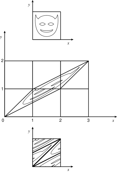
Figure 2: The Arnold cat map.

The baker’s map and the Arnold cat map are two simple examples of what are called hyperbolic dynamical systems. Briefly, and somewhat loosely stated, hyperbolic dynamical systems are defined by the action of some dynamical transformation, ${\bf S}$ on a phase-space $\Gamma$, such that: (a) one can identify stable and unstable directions in $\Gamma$, under the action of ${\bf S}$, with negative and positive Lyapunov exponents, all bounded away from zero; (b) the stable and unstable manifolds (lines, surfaces, etc.) are continuous functions of the variables that define the phase space, and when the two manifolds intersect, they do so transversely; (c) the system is transitive, i.e., there exists some trajectory in the phase-space that is dense on the phase-space; and (d) for maps, i.e., for dynamical systems where ${\bf S}$ acts only at discrete times, there are no directions in phase-space with a Lyapunov exponent of zero, while for “flows”, i.e. systems where ${\bf S}$ depends upon a continuous time parameter, the only direction in $\Gamma$ with a zero Lyapunov exponent is the direction of the flow. Clearly the baker’s map and the Arnold cat map are hyperbolic maps. A typical flow that one might examine for hyperbolicity is the motion of a phase point on surfaces of constant energy for a system of interacting particles.

2.3 Ergodic and mixing systems

The baker’s map and the Arnold cat map are also examples of dynamical systems which are ergodic and mixing. Ergodicity is the property of a dynamical system that the time average of any integrable function of the phase-space variables will be equal to the ensemble average of this function, the average taken with respect to an appropriate time translation invariant, equilibrium measure. That is, if $f(\Gamma)$ is an integrable function, then

$$\lim_{n\to\infty}\frac{1}{n}\sum_{j=o}^{n-1}f({\bf S}^{j}\Gamma)=\int f(\Gamma)\,\mu(d\Gamma),$$ (21)

where $\mu(A)$ is a measure that is invariant, i.e., $\mu(A)=\mu({\bf S}^{-1}A)$ for any non-trivial set $A$, and ergodic, meaning that it is impossible to divide the whole phase-space into two invariant sets, each of positive measure. It is generally assumed, but not always proved, that our systems possess a unique ergodic measure. Students of statistical mechanics will naturally associate the idea of an ergodic system with the name of Boltzmann who used this idea to base equilibrium statistical mechanics on the laws of mechanics.

Much of equilibrium statistical mechanics can be based on the laws of large numbers, and strict ergodicity, in the sense of Boltzmann, is not that essential. However, non-equilibrium statistical mechanics requires some deep underpinnings from mechanics, or from the theory of stochastic processes. Here we take the point of view that Hamiltonian mechanics is all that is needed, but that is certainly not the only possible point of view. For non-equilibrium statistical mechanics, it is useful to explore an idea of Gibbs, which is called the mixing property of a dynamical system. Mixing systems are always ergodic, but the reverse is not always true. To define a mixing system, we consider two arbitrary sets in the phase-space, $A$ and $B$, say, both of nonzero measure, and the evolution of the set $A$ in time. Suppose after $n$ iterations of the map ${\bf S}$ the set $A$ has moved to ${\bf S}^{n}A$, then the system is mixing if

$$\lim_{n\to\infty}\frac{\mu(B\cap{\bf S}^{n}A)}{\mu(B)}=\frac{\mu(A)}{\mu(\Gamma)},$$ (22)

where $\mu(\Gamma)$ is the measure of the entire phase-space, such as the unit square for the baker’s map or the cat map, or the constant energy surface for a more general system. The mixing condition simply means that the time evolution of a set in phase-space is such that, in a coarse grained sense, it gets uniformly distributed, with respect to the measure $\mu$, over the entire phase-space. It can be proved rather easily that for a mixing system, non-equilibrium averages of integrable functions $f$ will approach their equilibrium values in the course of time.

2.4 The approach to equilibrium

A nice illustration of the approach to equilibrium, as provided by baker or cat maps, is to consider the behavior in time of reduced distribution functions. That is, if we think of the unit square, again, as a phase space, then we can define a phase-space distribution function, $\rho_{n}(x,y)$, as a function of the number of iterations of the map, $n$, and the coordinates $x$ and $y$. The phase-space distribution function satisfies a discrete-time version of the Liouville equation, which is a form of the Frobenius-Perron equation for area preserving maps. The appropriate equation is

$$\rho_{n}(x,y)=\rho_{n-1}({\bf B}^{-1}(x,y)),$$ (23)

which, written out in full detail, becomes

$$\rho_{n}(x,y) = \rho_{n-1}(x/2,2y)\,\,\,{\mbox{for}}\,\,0\leq y<1/2$$ (24)

$$= \rho_{n-1}((x+1)/2,2y-1)\,\,\,\,{\mbox{for}}\,\,1/2\leq y<1.$$

A similar, but somewhat more complicated equation could be given for the Arnold cat map, but we will not use it here.

For these simple two dimensional models, a reduced distribution function is obtained by integrating the distribution function over one of the two phase-space variables, $x$ or $y$. This integration is motivated by the fact that for a system of $N$ particles, we are not particularly interested in the full $N$-particle distribution function, but rather in the one or two-particle distribution functions that can be used to evaluate the macroscopic quantities of interest, such as mass, momentum, and energy densities. Since our simple maps have only two coordinates, we can only consider the very simple case where a reduced distribution function is obtained by integrating over one of the coordinates. For the baker’s map we will construct the distribution function for the density of points in the $x$-direction, for reasons that will become clear as we proceed. That is, we define a reduced distribution function $W_{n}(x)$ by

$$W_{n}(x)=\int_{0}^{1}dy\,\rho_{n}(x,y).$$ (25)

Using Eq. (24), we can easily obtain a difference equation for $W_{n}(x)$, as

$$W_{n}(x)=\frac{1}{2}\left[W_{n-1}(\frac{x}{2})+W_{n-1}(\frac{x+1}{2})\right].$$ (26)

Figure 3: The projection, $W(x,n)$, onto the $x$-coordinate, of the phase-space distribution function for the Arnold cat map.

Figure 4: The projection, $G(y,n)$, onto the $y$-coordinate, of the phase-space distribution function for the Arnold cat map.

This equation is, among other things, the Frobenius-Perron equation for the one-dimensional map, $x^{\prime}=2x$ (mod $1$), on the interval $(0,1)$. What is more important here, though, is that except for very special initial values for $W_{0}(x)$, such as Dirac delta functions on the periodic points of the map, $W_{n}(x)$ approaches a constant, independent of $x$, as $n\to\infty$. This may be proved in a number of ways, but may be understood most simply by just drawing some possible functional forms for $W_{0}(x)$ and follow what happens to them after a few iterations of Eq. (26). A standard procedure is to make a Fourier expansion of $W_{0}(x)$, and to notice that only the constant term remains as the number of iterations gets large. The approach to equilibrium in this simple system can be associated with the properties of the expanding manifold in our simple two-dimensional phase-space. Because of the stretching of regions in phase-space in the unstable directions, functions defined on the unstable manifold will get “smoothed out” in the course of time, much the same way that a ball of dough gets smoother and smoother along the direction that the baker stretches it. The initial wrinkles in the phase-space distribution function will not get smoothed out along the stable direction, on the contrary, they typically will get more and more wrinkled as the system evolves. From these considerations we can see that the integration of the phase-space distribution over the stable direction in Eq. (25) was not chosen accidentally; had we integrated over $x$ instead, we would not have obtained an equation with a nice equilibrium solution as $n\to\infty$. In fact, a typical initial distribution will become smooth in the expanding directions but very striated in the contracting directions. However, eventually it will look uniform on a coarse grained scale, consistent with the mixing behavior of the baker’s map.

The connection between the approach to equilibrium and the expanding direction of a measure preserving map can be further explored by considering the Arnold cat map. Here, the expanding direction is along a line that is not aligned along either of the coordinate axes. One would expect that for this model a projection of the phase-space distribution function along either the $x$-axis, or the $y$-axis, would approach an equilibrium value. That this is so can be seen from a simple computer calculation. We start with a phase-space distribution that is concentrated in a small region $0\leq x,y\leq 0.1$. We then follow the evolution in time of $x$ and $y$ projections of the distribution function. In Figs. 3 and 4 we can easily see that these distribution approach constant values after three or four iterations of the map, much before the entire phase-space distribution is smooth, even on a reasonably coarse grained scale, which for this arrangement takes eight to ten iterations. This observation may be generalized: reduced distribution functions on some lower dimensional projection of phase-space will always become smooth under the dynamics, unless the projected space is entirely spanned by stable directions (hence is some subset of the stable manifold).

Figure 5: The Boltzmann $H$-functions $H_{W}(n)$ and $H_{G}(n)$, obtained by using $W(x,n)$ and $G(y,n)$ respectively.

Not only does one see an approach to an equilibrium distribution for the projected distribution functions for these maps, one also sees that a suitably defined Boltzmann $H$-function decreases monotonically as the number of iterations increases. This is illustrated in Fig. 5 for the Arnold cat map, for both projected distribution functions, starting from the same initial state as described above. The figure shows the $H$-function for both projections, as calculated on a computer. For the baker’s map, we can easily show the monotonic decrease in the $H$ function analytically. To do this we define the $H$-function by

$$H(n)=\int_{0}^{1}dx\,W_{n}(x)\,\ln W_{n}(x).$$ (27)

If we now use the recursion relation for $W_{n}(x)$, Eq. (26), we find that

$$\!\!\!\!H(n+1)=\int_{0}^{1}dx\,W_{n+1}(x)\,\ln W_{n+1}(x)$$

$$\!\!\!\!\quad=\int_{0}^{1}dx\frac{1}{2}\left[W_{n}(\frac{x}{2})+W_{n}(\frac{x+1}{2})\right]\ln\left\{\frac{1}{2}\left[[W_{n}(\frac{x}{2})+W_{n}(\frac{x+1}{2})\right]\right\}$$

$$\!\!\!\!\quad\leq\frac{1}{2}\int_{0}^{1}dx\,\left[W_{n}(\frac{x}{2})\ln W_{n}(\frac{x}{2})+W_{n}(\frac{x+1}{2})\ln W_{n}(\frac{x+1}{2})\right]$$

$$\!\!\!\!\quad=H(n).$$ (28)

The inequality in Eq. (28) follows from the fact that $f[(a+b)/2]\leq[f(a)+f(b)]/2$ if $f(x)=x\ln x$. That is, a chord connecting two points on the curve $x\ln x$ lies above the curve. Thus we see that the $H$ function decreases with time until $W_{n}(x)$ becomes a constant.

We conclude this discussion with a few remarks. For the baker’s map and the Arnold cat map, admittedly “toy” models, highly simplified versions of $N$ particle systems, with almost trivial phase-spaces, we have been able to derive irreversible equations and $H$-theorems with a minimum of assumptions. We have associated the approach to equilibrium of projected distribution functions with the existence of unstable manifolds for the dynamics in phase-space, and the fact that the projection is not orthogonal to the unstable directions. In a more general context, such as a corresponding, but not yet possible, dynamical derivation of the Boltzmann transport equation, we would expect that the approach to equilibrium, seen here for baker and Arnold cat maps, would correspond to the approach to a local equilibrium state in the fluid. In such a local equilibrium state, the system has equilibrium values for density, temperature, and local mean velocity over distances of a few mean free paths. Then much slower hydrodynamic processes with a different kind of dynamics govern the approach to an overall equilibrium state for the entire fluid.

2.5 The Kolmogorov-Sinai entropy

We next turn to a brief discussion of an important quantity that characterizes both deterministic chaos of the type we have been studying, as well as Markov, stochastic processes. This quantity is called the Kolmogorov-Sinai (KS) entropy. For a deterministic system it measures the rate at which information is gained about the initial state of a system. That is, suppose that we know that the initial phase point of our system is in some small region of $\Gamma$-space of dimension $\varepsilon$ on a side, and that we cannot resolve the location in $\Gamma$-space to any better precision. Consider now the evolution of this small volume element in $\Gamma$-space. For a system with non-zero Lyapunov exponents, this small volume will get exponentially stretched along the expanding directions. After some time this stretching will make some sides exponentially longer than the initial value $\varepsilon$, typically of length $\varepsilon\exp(\lambda_{i}t)$, where $\lambda_{i}$ is one of the positive Lyapunov exponents. Since we can resolve points in $\Gamma$-space to within a distance of $\varepsilon$ in any direction, we can now determine which of many small regions, of dimension $\varepsilon$ on a side, our system is in at time $t$. Then by inferring where this region came from in the initial volume, we learn more about the initial location of the phase point. Although it requires some careful analysis to prove, it is not difficult to imagine that there is some direct relation between the positive Lyapunov exponents and the KS entropy, $h_{KS}$. In fact for a closed, hyperbolic system, Pesin has proved that the relation is as direct as our discussion above would imply, namely,

$$h_{KS}=\sum_{\lambda_{i}>0}\lambda_{i}.$$ (29)

A deep and interesting fact is that at least one way to prove Pesin’s result (which we will not do here) depends on the fact that hyperbolic systems can be mapped onto Markov stochastic processes. That is, for such systems, with baker and Arnold cat maps as simple examples, one can represent the dynamics to within any arbitrary degree of precision, as a Markov process. Such Markov processes have a measure of their own information entropy, a quantity which measures the degree of uncertainty in the next outcome of the stochastic process. One can show that the information entropy, suitably defined, of the stochastic representation of a hyperbolic dynamical system is equal to the KS entropy of the system. This is one of the deep results of dynamical systems theory, which provides a firm mathematical basis for the correspondence of hyperbolic dynamical systems with Markov processes. It expresses the fact that from the point of view of mathematical analysis, at least, there is no real difference between a Newtonian, hyperbolic dynamical system with a finite KS entropy, and a Markov stochastic process with equal values of the information entropy. From the point of view of physics there is a big difference, of course. The central idea of the physical approach we take is to show that Newtonian dynamical systems are sufficiently hyperbolic to behave as if they were Markov stochastic systems and in consequence all important properties of Markov systems apply to dynamical systems, too.

An important first step is to show that some useful models of physical systems have positive Lyapunov exponents and a finite, positive KS entropy per particle. In the next sections we will show how methods of statistical mechanics can be used to calculate Lyapunov exponents and KS entropies of some simple many-particle systems—gases of hard spheres in $d$ dimensions, where $d=2,3$. Before doing so, however, we briefly turn our attention to an application of the ideas of this section to non-equilibrium statistical mechanics.

2.6 The escape-rate formalism for transport coefficients

We conclude this section with a discussion of a formal relation between the transport coefficients that characterize hydrodynamic processes in fluid systems, and the chaotic properties, such as Lyapunov exponents and KS entropies that characterize the underlying dynamical behavior of the fluid. The relation of interest here is called the “escape-rate” formula for transport coefficients and is due to Gaspard, Nicolis, and co-workers[6, 7]. It applies to those fluids which can be considered to be classical, transitive, hyperbolic dynamical systems. While we do not know with certainty if any models of fluid systems satisfy this hyperbolicity requirement, we can suppose, as a working hypothesis, that generic fluid systems are well described as transitive hyperbolic systems, and then explore the consequences that result. This hypothesis has been assumed by almost all workers in this field, but its most satisfactory articulation was provided by Cohen and Gallavotti in their study of non-equilibrium fluctuations in thermostatted systems[8].

To illustrate the escape-rate formula, we consider only the case of particle diffusion in an array of fixed scatterers, and refer to the literature for more general cases[7, 9]. We suppose that a collection of particles is moving in a region $R$ in space, and that there is also a collection of fixed scatterers placed in $R$, as illustrated in Fig. (6). We suppose that the size of $R$ is characterized by a length $L$ which is much larger than the typical mean free path of the particles moving in $R$. For simplicity we suppose that the moving particles do not interact with each other but only with the scatterers, and that the scatterers do not “trap” the moving particles in regions of microscopic or macroscopic size. In order to provide a non-equilibrium situation which would exhibit the diffusive properties of this arrangement, we suppose that $R$ is surrounded by absorbing boundaries such that if a particle crosses the boundary of $R$ from the interior, it is absorbed and lost to the system.

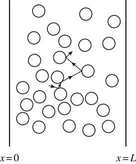
Figure 6: A slab geometry for diffusion in a system of moving particles is an array of fixed scatterers, with absorbing boundaries.

Under most circumstances , the classical, macroscopic dynamics of this process is described by the diffusion equation

$$\frac{\partial n(\vec{r},t)}{\partial t}=D\nabla^{2}n(\vec{r},t),$$ (30)

where $n(\vec{r},t)$ is the density of moving particles at time $t$ at point $\vec{r}$, and $D$ is the coefficient of diffusion of the moving particles for this system. The absorbing boundary conditions require that $n(\vec{r},t)=0$ on the boundaries. While the exact solution of Eq. (30) depends on the geometry of the system, one can easily see that for long times, the total number of particles in the system decays with time as

$$N(t)=\int_{R}d\vec{r}n(\vec{r},t)\simeq N(t=0)\exp[-DA\,t/L^{2}],$$ (31)

where $A$ is a factor of order unity that depends on the geometry of the region $R$, $D$ is the diffusion coefficient, and $L$ is the characteristic size of $R$. We see that this macroscopic process is characterized by an exponential escape of particles from $R$, with an escape-rate, $\gamma_{mac}=DA/L^{2}$. There is a corresponding microscopic description of the escape process based upon the properties of the trajectories of the particles moving in the array of scatterers. There is a set of initial points in the phase space for the moving particles which are associated with trajectories that never leave the system for either the forward or time reversed motion. This set of points is called a repeller and denoted by ${\cal R}$, and it is invariant, in the sense that any time-translation of this set of points is the set ${\cal R}$ itself. Further, the repeller usually forms a fractal set in phase space with zero Lebesgue measure. Simple examples of repellers can be found in most books on chaos theory[1, 3]. It is possible to consider the dynamical properties of the trajectories on the repeller, and to define the Lyapunov exponents, $\lambda_{i}({\cal R})$, and the KS entropy, $h_{KS}({\cal R})$, of such trajectories[9, 10, 11]. For transitive hyperbolic systems, one finds that the sum of the positive Lyapunov exponents on the repeller is not equal to the KS entropy as would be the case for closed systems according to Pesin’s theorem, but that the two quantities differ by an amount equal to the rate at which the other trajectories escape from the system, which we denote by $\gamma_{mic}$. That is

$$\gamma_{mic}=\sum_{\lambda_{i}>0}\lambda_{i}({\cal R})-h_{KS}({\cal R}).$$ (32)

Now we make the reasonable conjecture that the microscopic and the macroscopic escape-rates are equal, which leads to an expression for the diffusion coefficient $D$ given by

$$D=\lim_{L\rightarrow\infty}\frac{L^{2}}{A}\left[\sum_{\lambda_{i}>0}\lambda_{i}({\cal R})-h_{KS}({\cal R})\right],$$ (33)

where we have taken the large system limit in order to remove terms of higher order in $1/L$ resulting from deviations of the actual dynamics from the diffusion law. In the event that the limit on the right hand side of Eq. (33) exists, one has an expression for a macroscopic transport coefficient in terms of microscopic dynamical quantities. The escape-rate formalism has been applied by Gaspard and Baras[12] to determine the diffusion coefficient of a particle moving in a dense array of hard disk scatterers, where the centers of the scatterers are placed at the vertices of a triangular lattice, and by van Beijeren, Dorfman, and Latz, to determine the KS entropy on the repeller of a dilute, random Lorentz gas with hard disk or hard sphere scatterers[13].

3 Largest Lyapunov exponent of a gas of hard spheres at low density

3.1 The hard sphere gas

Often the calculation of chaotic characteristics of a system can only be done numerically. It would be preferable if one could at least find approximate values for such quantities using more analytical methods, and thus gain some insight into the relevant physical processes. For the Lorentz Gas at low densities, this was done by Dorfman, Van Beijeren and others [15, 13, 16, 17]. Here we present a calculation of the largest Lyapunov exponent for a system that is closer to a real gas, namely a dilute hard sphere gas. A brief presentation of this calculation can be found in Ref. [18].

We take $N$ hard spheres in a volume $V$, in $d$ dimensions. The diameter of the hard spheres is $\sigma$, the reduced density is defined as the dimensionless number $\tilde{n}=N\sigma^{d}/V$. We work in the thermodynamic limit $N,V\rightarrow\infty$, keeping $\tilde{n}$ fixed (but small). In this limit we need not be concerned with boundary conditions, but one may think of periodic boundary conditions, which have been used in Molecular Dynamics simulations to which we will eventually compare our results.

The phase-space of the hard sphere gas consists of the positions $\{\vec{r}_{i}\}$ and velocities $\{\vec{v}_{i}\}$ of all $N$ particles. To calculate the largest Lyapunov exponent, denoted here by $\lambda_{+}$, we need to consider two infinitesimally close trajectories in phase-space, $\Gamma=(\vec{r}_{1},\vec{v}_{1},\ldots,\vec{r}_{N},\vec{v}_{N})$ and $\Gamma+\delta\Gamma$ $=$ $\Gamma$ $+$ $(\delta\vec{r}_{1},\delta\vec{v}_{1},\ldots,\delta\vec{r}_{N},\delta\vec{v}_{N})$. The dynamics of the $\delta\vec{r}_{i}$ and $\delta\vec{v}_{i}$ is found from linearizing the dynamics of $\vec{r}_{i}$ and $\vec{v}_{i}$, which consists of a sequence of free flights and binary collisions. In free flight, there are continuous changes,

$$\dot{\vec{r}_{i}} = \vec{v}_{i}$$

$$\dot{\vec{v}_{i}} = 0$$

$$\dot{\delta\vec{r}_{i}} = \delta\vec{v}_{i}$$

$$\dot{\delta\vec{v}_{i}} = 0,$$ (34)

and at collisions the values of the two particles $i$ and $j$ change discontinuously according to:

$$\vec{r}^{\,\prime}_{j} = \vec{r}_{j}$$

$$\vec{v}^{\,\prime}_{j} = \vec{v}_{j}+(\vec{v}_{ij}\cdot\hat{\sigma})\hat{\sigma}$$

$$\delta\vec{r}^{\,\prime}_{j} = \delta\vec{r}_{j}+(\delta\vec{r}_{ij}\cdot\hat{\sigma})\hat{\sigma}$$

$$\delta\vec{v}^{\,\prime}_{j} = \delta\vec{v}_{j}+(\delta\vec{v}_{ij}\cdot\hat{\sigma})\hat{\sigma}+\mbox{\boldmath$Q$}(\delta\vec{r}_{i}-\delta\vec{r}_{j}).$$ (35)

Primes are used to denote values right after the collision. $\vec{v}_{ij}=\vec{v}_{i}-\vec{v}_{j}$ is the relative velocity and $\hat{\sigma}=(\vec{r}_{i}-\vec{r}_{j})/\sigma$ is the collision parameter. $Q$ is the matrix[18]

$$\mbox{\boldmath$Q$}=\frac{\left[(\hat{\sigma}\cdot\vec{v}_{ij})\mbox{\boldmath$1$}+\hat{\sigma}{\vec{v}_{ij}}\right]\cdot\left[(\hat{\sigma}\cdot\vec{v}_{ij})\mbox{\boldmath$1$}-\vec{v}_{ij}{\hat{\sigma}}\right]}{\sigma(\hat{\sigma}\cdot\vec{v}_{ij})}.$$ (36)

The non-dotted products of vectors are dyadic products and $1$ is the identity matrix.

Our approach will be based on kinetic theory. We are concerned with the distribution of $(\vec{r},\vec{v},\delta\vec{r},\delta\vec{v})$ as a function of time. For low densities, the evolution of the distribution function $f$ is described by a kinetic equation[19]. This equation is based on the assumption that two colliding particles are uncorrelated, so that the probability of a collision between a particle with $(\vec{r}_{1},\vec{v}_{1},\delta\vec{r}_{1},\delta\vec{v}_{1})$ and one with $(\vec{r}_{2},\vec{v}_{2},\delta\vec{r}_{2},\delta\vec{v}_{2})$ is proportional to the product $f(\vec{r}_{1},\vec{v}_{1},\delta\vec{r}_{1},\delta\vec{v}_{1})$ $f(\vec{r}_{2},\vec{v}_{2},\delta\vec{r}_{2},\delta\vec{v}_{2})$.

The kinetic equation can, unlike the ordinary Boltzmann equation, be expanded in powers of $1/|\ln\tilde{n}|$ to get the low density behavior of $f$, and thus of $\lambda_{+}$. We will take a different but roughly equivalent approach, we will derive the effective dynamics of the $\delta\vec{r}_{i}$ and $\delta\vec{v}_{i}$ for low densities, and use that to write down a kinetic equation.

3.2 Low density dynamics – Clock model

The main characteristics of the low density region is the typically long free flight time $\tau$ of an individual particle between collisions, compared to the time it would take two transparent hard spheres to cross each other. If $v_{0}$ is the typical thermal velocity, the latter is $\sigma/v_{0}$, while $\tau\approx 1/(v_{0}\sigma^{d-1}N/V)=\sigma/(v_{0}\tilde{n})$. Thus $\tilde{n}$ is the small parameter.

Just before a collision at time $t$ the $\delta\vec{r}_{i}(t)$ will be

$$\delta\vec{r}_{i}(t)=\delta\vec{r}_{i}(t_{0})+\delta\vec{v}_{i}(t_{0})\tau_{i}\,,$$ (37)

if $t_{0}$ is the time of the previous collision and $\tau_{i}$ is the (large) free flight time $t-t_{0}$. Suppose that initially $\delta\vec{r}_{i}(t_{0})/\sigma$ and $\delta\vec{v}_{i}(t_{0})/v_{0}$ are of the same order, then just before collision,

$$\delta\vec{r}_{i}=\tau_{i}\left[\delta\vec{v}_{i}+{\cal O}(\tilde{n})\right].$$

We insert this into the collision rules and neglect the terms of relative order ${\cal O}(\tilde{n})$:

$$\delta\vec{r}^{\,\prime}_{j} \approx \tau_{j}\delta\vec{v}_{j}+\{(\tau_{i}\delta\vec{v}_{i}-\tau_{j}\delta\vec{v}_{j})\cdot\hat{\sigma}\}\hat{\sigma}$$

$$\delta\vec{v}^{\,\prime}_{j} \approx \mbox{\boldmath$Q$}(\tau_{i}\delta\vec{v}_{i}-\tau_{j}\delta\vec{v}_{j}).$$ (38)

Using Eq. (36), we see that $\delta\vec{r}^{\,\prime}_{i}/\sigma$ and $\delta\vec{v}^{\,\prime}_{i}/v_{0}$ are both of order $(\delta\vec{v}_{i}-\delta\vec{v}_{j})/{v_{0}\tilde{n}}$, and are of the order of the ratio of the mean free time to the time it takes to traverse a particle diameter. For a dilute gas, this ratio is large and terms of relative order $\tilde{n}$ can be neglected. In this way we have eliminated the $\delta\vec{r}_{i}$ from the $\delta\vec{v}_{i}$ dynamics.

The neglected terms were of relative order $\tilde{n}$, relative to either $\tau_{i}\delta\vec{v}_{i}$ or $\tau_{j}\delta\vec{v}_{j}$. These two are not necesarily of the same order. Now, if one of them is one or more orders of $\tilde{n}$ higher than the other, we should also neglect it. If they are both of the same order, we should keep both. To know which terms to neglect, we have to keep track of the orders of $\tilde{n}$ in $\delta\vec{v}_{i}$. For that purpose, we define

$$\delta\vec{v}_{i}=v_{0}(\tilde{n})^{-k_{i}}\hat{e}_{i},$$ (39)

where $\|\hat{e}_{i}\|=1$. The number $k_{i}$ counts the number of orders of $\tilde{n}$ and we will call this the clock value of particle $i$. The clock values are real numbers at this point, but later will be approximated by integers. Inserting Eq. (39) into Eq. (38), we can get the clock values $k^{\prime}_{i}$ and $k^{\prime}_{j}$ after collision. Since, to leading order in density, $\delta\vec{v}^{\,\prime}_{i}$ and $\delta\vec{v}^{\,\prime}_{j}$ differ only in sign, $k^{\prime}_{i}=k^{\prime}_{j}=k^{\prime}$, with

$$k^{\prime}=\frac{1}{-\ln{\tilde{n}}}\ln\|\mbox{\boldmath$Q$}(\tau_{i}\delta\vec{v}_{i}-\tau_{j}\delta\vec{v}_{j})\|.$$

Both $\tau_{i}$ and $\tau_{j}$ are typically of order $\sigma/(v_{0}\tilde{n})$. This means that if $k_{i}>k_{j}$, we should neglect the term with $\delta\vec{v}_{j}$, and if $k_{i}<k_{j}$, we should neglect the other term. This yields:

$$k^{\prime}=k_{D}+\frac{1}{-\ln{\tilde{n}}}\ln\|\mbox{\boldmath$Q$}\tau_{D}\hat{e}_{D}\|,$$

where $D=i$ if $k_{i}>k_{j}$, and $D=j$ otherwise. Particle $D$ is called the dominant particle. Using the property $\tau_{D}={\cal O}(\sigma/(v_{0}\tilde{n}))$ and the explicit form of $Q$ from Eq. (36), one gets

$$k^{\prime}=k_{D}+1+{\cal O}(\frac{1}{\ln\tilde{n}}).$$

So far we have ignored the possibility that $k_{i}=k_{j}$. But the resulting correction in fact only contributes to the ${\cal O}(1/\ln\tilde{n})$ part.

Differences in the number of collisions suffered by different particles, cause the clock values to not be all the same, even if they were so initially. They are indispensible for determining the magnitudes of postcollisional velocity deviations. But in fact no more is needed! For if we know how fast the clock values grow, we know the linear growth of $\ln\|\delta\vec{v}\|$, which is precisely the largest Lyapunov exponent. So we define the clock speed as

$$w=\lim_{t\rightarrow\infty}\frac{<k(t)>}{\bar{\nu}t},$$

in which $<k>$ is the average clock value and $\bar{\nu}$ is the average collision frequency. Because we extracted $\bar{\nu}$, which is ${\cal O}(\tilde{n})$, this clock speed is of order 1.

The Lyapunov exponent is related to $w$ via

$$\lambda_{+}=-w\bar{\nu}\ln\tilde{n}.$$

The clock speed $w$ will be calculated in an expansion in $1/|\ln\tilde{n}|$. The leading order for low density, calculated in the next section, is a non-trivial constant. This behavior of $\lambda_{+}$ as a function of density had been conjectured already by Krylov[20], however without a nontrivial prefactor $w$. A first estimate of $w$ was made by Stoddard and Ford[21], who got $w=\ln N$. This would mean that there is no thermodynamic limit for the Lyapunov exponent. Some numerical simulations[22] have been interpreted as supporting the logarithmic divergence with $N$, but with a prefactor much smaller than $1$. However, we will find a finite thermodynamic limit for $w$ and show that, even in a mean-field approach that fully ignores local density fluctuations, it approaches this thermodynamic value so slowly that in the range of particle numbers accessible to simulations one could not distiguish between saturation or slow but steady increase.

3.3 Kinetic approach

For low densities, we may describe the effective dynamics of the clock values by

$$k_{i}^{\prime}=k_{j}^{\prime}=\max(k_{i},k_{j})+1,$$ (40)

where the collision pairs $(i,j)$ are chosen completely randomly with Poisson distributed collision times. The model with this dynamics we will call the clock model. For simplicity we will consider integer clock values only, though this restriction is by no means necessary or important. The clock speed $w$ found in this model gives the leading term in the density expansion of the Lyapunov exponent:

$$\lambda_{+}=w\bar{\nu}\left[-\ln\tilde{n}+{\cal O}(1)\right].$$ (41)

A distribution function $f_{k}(t)$ will denote the fraction of particles having clock value $k$ at time $t$. From the dynamics specified above we can derive an equation for the distribution function $f_{k}(t)$ of clock values. We expect the clock values to grow linearly with time. If they all grow at the same rate, we have

$$f_{k}(t)=g(k-w\bar{\nu}t),$$

with $w$ as defined before, because

$$\lim_{t\rightarrow\infty}\frac{1}{\bar{\nu}t}\sum_{k=-\infty}^{\infty}g(k-w\bar{\nu}t)k=\lim_{t\rightarrow\infty}\frac{1}{\bar{\nu}t}\sum_{x=-\infty}^{\infty}g(x)(x+w\bar{\nu}t)=w.$$

So once we have a kinetic equation for $f_{k}(t)$, we will look for these propagating solutions.

Consider the contributions to $\frac{\partial f_{k}}{\partial t}$ from collisions in which a clock value $k$ is lost. In each collision where a particle with $k$ enters, the $k$ gets lost, so the fraction of particles with $k$ decreases at a rate $\bar{\nu}f_{k}(t)$ due to these processes. There are also processes which increase the fraction of particles having $k$. For these the larger incoming clock value should be $k-1$. We have to distiguish collisions with equal incoming clock values, both $k-1$, from ones with different incoming clock values $k-1$ and $l$. The rate for the latter type of collisions is $\bar{\nu}f_{k-1}\sum_{l=-\infty}^{k-2}f_{l}$. For the former ones the rate is only $1/2$ $\bar{\nu}f^{2}_{k-1}$, because the two particles are drawn from the same fraction $f_{k-1}$, and it doesn’t matter in which order they are picked. In either case the number of particles with clock value $k$ increases by two, so we get the kinetic equation:

$$\frac{\partial f_{k}(t)}{\partial\bar{\nu}t}=-f_{k}(t)+f^{2}_{k-1}+2f_{k-1}\sum_{l=-\infty}^{k-2}f_{l}.$$

We scale out $\bar{\nu}$ by defining a new time variable $\tau=\bar{\nu}t$. The equation is simplified further by replacing the fraction $f_{k}$ of particles having clock value $k$, by the fraction $C_{k}$ of particles that have clock values $k$ or less:

$$C_{k}(\tau)=\sum_{l=-\infty}^{k}f_{l}(\tau).$$

The kinetic equation then takes the short form:

$$\frac{\partial C_{k}}{\partial\tau}=-C_{k}+C^{2}_{k-1}.$$ (42)

3.4 Front propagation

Let us investigate the solutions of Eq. (42). We see that, given $C_{k-1}$ and the initial value of $C_{k}$, we can solve for $C_{k}$:

$$C_{k}(\tau)=e^{-\tau}\left[C_{k}(0)+\int_{0}^{\tau}e^{\tau^{\prime}}C^{2}_{k-1}(\tau^{\prime})d\tau^{\prime}\right].$$

If $C_{k}=0$ initially, it will remain zero, because $0\leq C_{k-1}\leq C_{k}$. We take initial conditions such that $C_{k<1}(0)=0$ and $C_{k>0}=1$, i.e. all particles have $k=1$. The solutions $C_{k}$ are all polynomials in $\exp(-\tau)$, but with increasing $k$ the order grows exponentially. Nonetheless, we calculated the $C_{k}$ up to $k=32$ using a computer program to handle the analytic manipulations. The $C_{k}$’s are plotted in Fig. 7 for $\tau=0,2,4,6$ and $10$.

Figure 7: Time evolution of the clock value distribution. All initial clock values are $0$.

We see in Fig. 7 that the initial distribution changes to some smoother shape, and moves to the right. After a while the shape seems to stay constant. We can now view Eq. (42) as describing a propagating front: $C\equiv 0$ is a stable phase and $C\equiv 1$ is an unstable phase. On the left we have the stable phase, on the right, the unstable phase and in between is the intermediate region called the front , that propagates to the right, into the unstable phase. The velocity at which it moves to the right is $w$. From Fig. 7 we see that for $\tau=10$, the speed is still increasing, and is about 3.8.

Front propagation into an unstable phase comes in two flavors[23]. In general, the instability of the unstable phase sets a velocity $w^{*}$ by which small perturbations propagate to the right. This velocity $w^{*}$ is determined from the linearized equation describing the front propagation around the unstable phase. For pulled fronts $w^{*}$ is the asymptotic velocity of any solution with an initial shape that is sufficiently steep. If, however, no solution of the full non-linear front equation with this velocity exists, or if it is unstable with respect to some nonlinear perturbation, the velocity is set by these non-linearities and the front is called pushed. In that case the velocity is higher than $w^{*}$. We will assume that in our case the front is pulled. As we do not know of a general criterion for deciding whether a front is pushed or pulled, we will use the results of computer simulations for the validation of our assumption.

We want to find a solution to Eq. (42) of the form

$$C_{k}(\tau)=F(k-w\tau)=F(x).$$

which means

$$-w\frac{dF(x)}{dx}=-F(x)+F^{2}(x-1).$$ (43)

Now $C$ is a positive, increasing function of $k$, bounded between $0$ and $1$. The function $F$ should have all these properties too. So we are looking for a solution of a form such as depicted in Fig. 8.

Figure 8: Clock value distribution as a propagating front

For a pulled front, we have to investigate the Eq. (43) linearized around the unstable phase. Writing $F=1-\Delta$, we get

$$-w\frac{d\Delta(x)}{dx}=-\Delta(x)+2\Delta(x-1)+{\cal O}(\Delta^{2}).$$ (44)

Given $w$, the asymptotic solution of Eq. (44) is given by a sum of exponentials[24]

$$\Delta(x)=\sum_{i}A_{i}e^{-\gamma_{i}x}.$$ (45)

The possible values of $\gamma_{i}$ are found by inserting $\exp(-\gamma x)$ into the linearized equation (in case of degeneracies, $A_{i}$ should be replaced by a polynomial in $x$). This gives $w$ as a function of $\gamma$:

$$w(\gamma)=(2e^{\gamma}-1)/\gamma.$$ (46)

The $\gamma_{i}$ may be complex, and, for given $w$, there are infinitely many of them. However, we know that $\Delta$ should be monotonic, so the most slowly decaying term in the sum should have a real positive $\gamma$.

From the plot of Eq. (46) in Fig. 9, we see that there are three cases: If $w$ is larger than some critical $w^{*}$, there are two $\gamma$’s, which are real and positive. If $w=w^{*}$ these two become degenerate and for $w<w^{*}$ they become complex. But for the slowest term to have complex $\gamma$ was not allowed by the condition of monotonicity of $F$: asymptotically the function would oscillate. So we conclude that, for the the Ansatz of a propagating front to work, the velocity should be at least $w^{*}$, the minimal $w$ from Eq. (46) for positive real $\gamma$. This value can be expressed in terms of Lambert’s $W$ function:

$$w^{*}=\frac{-1}{W(\frac{-1}{2e})}\approx 4.31107\ldots,$$

Figure 9: Velocity versus asymptotic decay rate $\gamma$.

and it is the velocity set by the instability that we mentioned before. So it is the velocity $w$ we were after. Its value is compatible with the estimate 3.8 from Fig. 7 (a lower value than 3.8 would not), which supports the assumption of a pulled front. This concludes the calculation of the leading order in Eq. (41) of the largest Lyapunov exponent in the infinite system limit within the framework of our clock model, but we still have to consider the effects of a finite number of particles.

3.5 Large finite $N$ effects

The kinetic equation works well in the thermodynamic limit, but to compare our results with simulations we need to correct for the effects of the finiteness of the number of particles. The clock model is very suitable for simple simulations. We take a set of $N$ integer numbers $\{k_{i}\}$. In each time step two of them are picked at random, and the collision rule in Eq. (40) is applied to them. We do this $T$ times. The average number of collisions per particle is then $2T/N$, because in each of the $T$ collisions two particles are involved. An estimate for the clock speed is the average clock value $\sum_{i}k_{i}/N$ divided by the average number of collisions per particle. For large $T$ this approaches the clock speed $w_{N}$, so

$$w_{N}=\lim_{T\rightarrow\infty}\frac{1}{2T}\sum_{i=1}^{N}k_{i}.$$

This simulation is not even a bad chacterization of what happens with the clock values in the hard sphere gas, because at low densities there is very little correlation between pairs of particles involved in subsequent collisions. It is very similar to the variant of the Direct Simulation Monte Carlo method used by Dellago and Posch[25] for the calculation of Lyapunov exponents in a “spatially homogeneous system”.

Clock speeds for different numbers of particles are plotted in Fig. 11. Each point is determined from a single run with 2000 collisions per particle. The sums of all clock values at 20 times were fitted to a linear function. The slope gave $w_{N}$, the error in the slope gave the error in $w_{N}$. The errors are always less than 0.5 percent. One sees that $w_{N}$ increases slowly with increasing $N$. It is possible that it saturates at the value of $4.311$, but this cannot yet be seen even for half a million particles.

A natural thought is that the $N$ dependence of $w$ is due to correlations between subsequent collisions: if two particles collide that already collided just before, or that had their clock values reset shortly before by particles that were roughly synchronized already, the gain in clock value of the ”slower” particle will be less than average. Hence the average clock speed is reduced. However, as we will see, the reduction in clock speed can be explained entirely on the basis of the linearized equation plus some simple bounds on its region of validity and this explanation does not seem to require any effects of correlated collisions.

In the head of the distribution, the finiteness of the number of particles becomes important when $f_{k}={\cal O}(1/N)$. For this reason, Brunet and Derrida[26] treat the finite $N$ effects by the introduction of a cutoff $\varepsilon=1/N$ in the equation, i.e. they modify the equation as soon as $f_{k}<\varepsilon$. They distinguish three regions: one where the non-linear behavior is dominant, one where the linear equation holds, and one where the cutoff is effective. By glueing the solutions in these regions together, one obtains a new $\varepsilon$-dependent front velocity.

The introduction of a cutoff in something that is supposed to be a distribution function, which is an average over realizations, seems hard to justify. A more satisfactory way to obtain it, is to shift all clockvalues in each realization such that the particle with the largest clock value has $x=0$, and then average the distribution function (this was also suggested by Kessler et al[27]). Then the cutoff occurs naturally.

For $x<0$ there is a region where we can use the linearized equation. We consider the leading term in Eq. (45):

$$\Delta\sim\frac{c}{N}e^{-\gamma_{0}x}.$$

The prefactor $c/N$ is obtained from the fact that $\Delta={\cal O}(1/N)$ at $x=0$ ($c$ is order $1$). The linear regime ends when $\Delta$ becomes of order $1$, so for $x=-\ln(\frac{N}{c})/\gamma_{0}$. This is illustrated in Fig. 10.

Figure 10: The cutoff at the head of the distribution and the linear regime.

In contrast with the infinite system, now we only have to demand monotonicity and positivity from the solution of the linearized equation in this interval of width $\ln(\frac{N}{c})/\gamma_{0}$. This means that a small imaginary value is allowed for the $\gamma$ in Eq. (45) with the smallest real part. We denote $\gamma=\gamma_{R}+i\gamma_{I}$. The consequential oscillations,

$$\Delta=a_{0}\,e^{-\gamma_{R}x}\cos(\gamma_{I}x+\phi),$$

should not cause sign changes in the function or its derivative. The derivative can be sign definite if at most half a wavelength fits in the interval, i.e. if at most

$$\gamma_{I}=\frac{\gamma_{R}\pi}{\ln(N/c)}.$$

For the leading behavior $c$ can be set to $1$. Positivity of $\Delta$ itself also poses an additional bound on $\gamma_{I}$, but this can be shown to be a higher order effect.

Figure 11: Effect of finite $N$ on the clock speed. Diamonds are the simulations; the solid line is the prediction Eq. (48); the dashed line is the asymptotic value $4.311\ldots$. The inset shows the linear behavior of $1/\sqrt{w_{0}-w_{N}}$ (plotted with error bars) as a function of $\ln N$. The solid line in both is the fit to the form in Eq. (49).

We expand $w(\gamma)$ around its minimum at $\gamma_{0}$:

$$w(\gamma)=w(\gamma_{0}+\delta\gamma)\approx w(\gamma_{0})+\frac{1}{2}w^{\prime\prime}\delta\gamma^{2}+\frac{1}{6}w^{\prime\prime\prime}\delta\gamma^{3}+\mbox{h.o.}\mbox{(higher orders)},$$

where $w^{\prime\prime}=\frac{d^{2}w}{d\gamma^{2}}(\gamma_{0})$ and $w^{\prime\prime\prime}=\frac{d^{3}w}{d\gamma^{3}}(\gamma_{0})$. $w$ is still real, so the imaginary part gives

$$0=\delta\gamma_{I}\left\{w^{\prime\prime}\delta\gamma_{R}+\frac{1}{6}w^{\prime\prime\prime}[3\delta\gamma_{R}^{2}-\delta\gamma_{I}^{2}]+\mbox{h.o.}\right\},$$

where $\delta\gamma=\delta\gamma_{R}+i\delta\gamma_{I}$. To first order this says that $w^{\prime\prime}\delta\gamma_{R}=\frac{1}{6}w^{\prime\prime\prime}\delta\gamma_{I}^{2}$: the shift in the real part of $\gamma$ is higher order compared to the imaginary part. The new velocity is written as $w=w_{0}+\delta w$, and $\delta w$ is obtained from the real part of equation Eq. (46) expanded to first order:

$$\delta w = \frac{1}{2}w^{\prime\prime}\left\{\delta\gamma_{R}^{2}-\delta\gamma_{I}^{2}\right\}+\frac{1}{6}w^{\prime\prime\prime}\left\{\delta\gamma_{R}^{3}-\delta\gamma_{R}\delta\gamma_{I}^{2}\right\}+\mbox{h.o.}$$ (47)

$$= -\frac{1}{2}w^{\prime\prime}\delta\gamma_{I}^{2}+\mbox{h.o.}=-\frac{w^{\prime\prime}\pi^{2}\gamma_{0}^{2}}{2\ln^{2}(N/c)}+\mbox{h.o.},$$

which coincides with Brunet and Derrida’s result (when $c$ is set to $1$). They however needed to consider how the linear region connects to the others, while we only need that $\Delta$ is of order $1$ at the border with the non-linear region. From Eq. (46), one can show that $w^{\prime\prime}\gamma_{0}^{2}=(w_{0}-1)$, so we find the result

$$w_{N}=w_{0}-\frac{(w_{0}-1)\pi^{2}}{2\ln^{2}(N/c)}.$$ (48)

In Fig. 11 the simulation results are plotted together with a fit. We calculate $\delta w^{-1/2}=1/\sqrt{w_{0}-w_{N}}$, with $w_{N}$ taken from the simulations, which should be a linear function of $\ln N$ for large $N$:

$$\delta w^{-1/2}\stackrel{{\scriptstyle N\rightarrow\infty}}{{\longrightarrow}}a+b\ln N.$$ (49)

Indeed this behavior is seen in the inset of Fig. 11. According to Eq. (48), $a=-\ln c$ and $b=\pi^{-1}\sqrt{2/(w_{0}-1)}=0.247\ldots$. The fit to the data shown in the inset yields $b=0.23\pm 0.01$, consistent with the theoretical prediction, and $a=-0.07\pm 0.07$. The value of $c$ corresponding to this $a$ is $c\approx 1.07$, so it is of order $1$ as expected.

The values from our simulations have been compared in Ref. [18] to molecular dynamics simulations of hard spheres, from which $w$ is found from a fit of $\lambda_{+}$ to the form Eq. (41). The values agreed very well with the simulations.

3.6 Further refinements

Comparing the results from high precision simulations of the clock model on the one hand and of hard disk systems with exactly the same number of particles and equal collision frequency on the other hand, one finds that the dimensionless clock speed $w$ in the latter is significantly higher than in the former; for a system of $10,000$ particles the clock model gives a $w$ of 4.05 $\pm$ 0.01, whereas the corresponding hard disk value is 4.47 $\pm$ 0.02. The cause of this difference is the velocity dependence of the collision frequency, which is an increasing function of speed. As a result particles in the head of the distribution tend to have a higher speed than average (a higher collision frequency enhances the clock value), resulting in a clock speed that is systematically higher than it would be in the case of a velocity independent collision frequency. The clock model does have a velocity independent collision frequency indeed, which explains the difference in $w$ between this model and the hard disk system.

An explicit calculation accounting for these effects and producing improved estimates for $w$ in hard disk systems will appear soon[28].

4 Kolmogorov-Sinai entropy of a gas of hard spheres at low density

In the previous section we reviewed the calculation by Van Zon and Van Beijeren of the largest Lyapunov exponent for a gas of hard disks at low densities. Here we will outline a related, but somewhat simpler calculation of the KS entropy of a gas of hard disks or of hard spheres at low density. This calculation, while not rigorous in a mathematical sense, is a strong indication of the chaotic behavior of such gases, and indicates that the chaoticity of a dilute hard disk or hard sphere gas persists in the thermodynamic limit.

The starting point is the same as in the previous section. It is important to note that the dynamics of a hard sphere system is exactly described as free motion of the particles, punctuated by instantaneous, binary collisions between some pair of particles. To describe this motion and the quantities we need for the KS-entropy, we consider the dynamical behavior of the positions and coordinates of all the particles in the gas, $(\vec{r}_{1},\vec{v}_{1},\vec{r}_{2},\vec{v}_{2},\ldots,\vec{r}_{N},\vec{v}_{N})$, as well as a set of deviation vectors which describe the motion of a pencil of nearby trajectories in phase-space, $(\delta\vec{r}_{1},\delta\vec{v}_{1},\ldots,\delta\vec{r}_{N},\delta\vec{v}_{N})$. The equations of motion for these quantities between the binary collisions are given by Eq. (34) and the changes of these quantities at a collision between particles $i$ and $j$ are given in Eqs. (35,36).

To proceed with the calculation of the KS-entropy, we will suppose that the Pesin formula holds, i.e., that the KS-entropy is the sum of the positive Lyapunov exponents. This sum can be obtained by considering the growth in time of the volume of the $dN$-dimensional projection of an arbitrary, infinitesimal volume in the full $2dN$-dimensional phase space. This observation requires some explanation, as follows. The typical rate of separation of two arbitrary, but infinitesimally close, points in phase-space, for a hyperbolic system, will be exponential and the rate will be given by the largest Lyapunov exponent. If we consider a typical two-dimensional, infinitesimal area in phase-space, then this area will grow exponentially with a rate determined by the sum of the two largest Lyapunov exponents. In other words, the exponential growth of a typical infinitesimal $n$-dimensional subvolume in phase space is determined by the sum of the $n$ largest Lyapunov exponents. Further, for a Hamiltonian system, the Lyapunov exponents come in plus-minus conjugate pairs, so that the sum of a conjugate pair of exponents is always zero. Consequently, the growth of an infinitesimal $dN$-dimensional subvolume is determined by the sum of the $dN$ non-negative Lyapunov exponents, and the volume of an infinitesimal $2dN$-dimensional volume remains constant, in accord with Liouville’s theorem.

For the typical $dN$ dimensional subvolume, we consider a volume formed by the projection of $2dN$ infinitesimal displacement vectors on velocity space, $(\delta\vec{v}_{1},\delta\vec{v}_{2},\ldots,\delta\vec{v}_{N})$. Given initial values for each of these vectors, as well as for all of the positions, $\vec{r}_{i}$, velocities, $\vec{v}_{i}$, and position deviation vectors, $\delta\vec{r}_{i}$, we can follow their evolution in time and, in principle at least, determine the time dependence of an infinitesmal volume element in velocity space, which we denote as $\delta{\cal V}(t)$. Then

$$h_{KS}=\sum_{\lambda_{i}\geq 0}\lambda_{i} = \lim_{t\to\infty}\frac{1}{t}\ln\frac{\delta{\cal V}(t)}{\delta{\cal V}(0)}$$ (50)

$$= \lim_{t\to\infty}\frac{1}{t}\int_{0}^{t}d\tau\frac{d\ln\delta{\cal V}(\tau)}{d\tau}$$

$$= \left\langle\frac{d\ln\delta{\cal V}(t)}{dt}\right\rangle.$$

The last line of Eq. (50) is based on the assumption (still unproven) that a gas of hard spheres is ergodic, so that time averages can be replaced by equilibrium averages taken with respect to a microcanonical ensemble. Here this average is denoted by angular brackets. Since we are considering a volume element in velocity space, we can use the fact that the velocity displacement vectors do not change during the free flight motion of the particles between the collisions, but do change at a collision. Under these circumstances, one can use elementary kinetic theory considerations to show that the final term on the right hand side of Eq. (50) is

$$\left\langle\frac{d\ln\delta{\cal V}(t)}{dt}\right\rangle=\left\langle\sum_{i<j}{\cal T}_{i,j}\ln\delta{\cal V}\right\rangle=\frac{N(N-1)}{2}\left\langle{\cal T}_{12}\ln\delta{\cal V}\right\rangle.$$ (51)

Here ${\cal T}_{12}$ is a binary collision operator, discussed in some detail in Refs. [29, 30], given by

$${\cal T}_{12}=\sigma^{d-1}\int_{\vec{v}_{12}\cdot\hat{\sigma}<0}d\hat{\sigma}|\vec{v}_{12}\cdot\hat{\sigma}|\delta(\vec{r}_{12}-\sigma\hat{\sigma})[{\cal P}_{\hat{\sigma}}(1,2)-1].$$ (52)

In Eq. (52), $d$ is the number of spatial dimensions of the system, $\sigma$ again is the diameter of the spheres, $\vec{r}_{12}=\vec{r}_{1}-\vec{r}_{2};\vec{v}_{12}=\vec{v}_{1}-\vec{v}_{2}$, and the operator ${\cal P}_{\hat{\sigma}}(1,2)$ is a substitution operator which replaces the precollision values, $\vec{r}_{1},\vec{v}_{1},\vec{r}_{2},\vec{v}_{2},\delta\vec{r}_{1},\delta\vec{v}_{1},\delta\vec{r}_{2},\delta\vec{v}_{2}$, by their post collision values, denoted with primes, given by Eqs. (35,36). The unit vector $\hat{\sigma}$ is an impact parameter, running in the direction of the line connecting the centers at collision and is integrated over a hemisphere corresponding to all allowed directions.

At this point it is useful to express the precollision quantities $\delta\vec{r}_{i}$ as

$$\delta\vec{r}_{i}=\delta\vec{r}_{i}(0)+\tau_{i}\delta\vec{v}_{i},$$ (53)

where $\delta\vec{r}_{i}(0)$ is the position displacement of particle $i$ just after its previous collision, and $\tau_{i}$ is the time between the previous collision of particle $i$ with some other particle, and the next collision involving particle $i$. To further simplify the expression for the KS-entropy, we now neglect, as in section 3, the initial displacement vectors, $\delta\vec{r}_{i}(0)$, when we calculate the change of the infinitesimal volume in velocity space at the $(1,2)$ collision in Eq. (51). This turns out to be a serious approximation. It leads to the correct value for the leading density term in $h_{KS}$, at low density, but the first order correction to this term is obtained incorrectly in this approximation. This can be repaired, but at the cost of a much longer and intricate calculation which we will present elsewhere.

If we insert $\delta\vec{r}_{1}=\tau_{1}\delta\vec{v}_{1}$ and $\delta\vec{r}_{2}=\tau_{2}\delta\vec{v}_{2}$ into the expression, Eq. (35), for the post collision velocity deviations for particles $1$ and $2$, we find that

$$\left[{\cal P}_{\hat{\sigma}}(1,2)-1\right]\ln\delta{\cal V}=\ln\frac{\delta{\cal V}^{\prime}}{\delta{\cal V}}=\ln|\det{\bf M}_{12}|,$$ (54)

where

$${\bf M}_{12}={\bf 1}-2\hat{\sigma}\hat{\sigma}-\frac{2T_{12}}{\sigma}\left[(\vec{v}_{12}\cdot\hat{\sigma}){\bf 1}-\vec{v}_{12}\hat{\sigma}+\hat{\sigma}\vec{v}_{12}-\frac{\vec{v}_{12}^{2}}{(\vec{v}_{12}\cdot\hat{\sigma})}\hat{\sigma}\hat{\sigma}\right].$$ (55)

In Eq. (55), $T_{12}=(\tau_{1}+\tau_{2})/2$ and ${\bf 1}$ is the unit matrix. The determinants are easily evaluated. For $d=2$, one finds

$$|\det{\bf M}_{12}|=1+\frac{2T_{12}|\vec{v}_{12}|}{\sigma\cos\phi},$$ (56)

where $\phi$ is the angle of incidence in the $1,2$ collision and ranges over the values $-\pi/2\leq\phi\leq\pi/2$. A similar calculation for $d=3$ shows that

$$|\det{\bf M}_{12}|=1+\frac{2T_{12}|\vec{v}_{12}|}{\sigma\cos\phi}(\cos^{2}\phi+1)+\left(\frac{2T_{12}|\vec{v}_{12}|}{\sigma}\right)^{2}.$$ (57)

To obtain the leading term in the density, for low density gases, we keep the highest power of the time in each of the expressions for the determinant. Further, at low densities we can compute the ensemble averages appearing in Eq. (50) by ignoring possible pre-collision correlations between particles $1$ and $2$, and using equilibrium values for the single-particle distribution functions appearing in the ensemble averages. In this way we find for $d=2$

$$h_{KS}/N = \frac{a}{2n}\int d\vec{v}_{1}\int d\vec{v}_{2}\int d\tau_{1}\int d\tau_{2}\int_{\vec{v}_{12}\cdot\hat{\sigma}<0}d\hat{\sigma}|\vec{v}_{12}\cdot\hat{\sigma}|\times$$ (58)

$$\times F_{1}(\vec{v}_{1},\tau_{1})F_{1}(\vec{v}_{2},\tau_{2})\ln T_{12}+\cdots,$$

where the normalized equilibrium single particle distribution functions, $F_{1}(\vec{v}_{i},\tau_{i})$ are given, in $d$ dimensions, by

$$F_{1}(\vec{v}_{i},\tau_{i})=n(\frac{\beta m}{2\pi})^{d/2}\nu(\vec{v}_{i})e^{-\beta m\vec{v}_{i}^{2}/2}e^{-\nu(\vec{v}_{i})\tau_{i}}.$$ (59)

Here $n$ is the number density of the gas, $\beta=(k_{B}T)^{-1}$, where $T$ is the gas temperature, and $k_{B}$ is Boltzmann’s constant, $\nu(\vec{v}_{i})$ is the equilibrium collision frequency for a particle with velocity $\vec{v}_{i}$. For two dimensions, the evaluation of the integrals leads directly to

$$h_{KS}/N=\frac{\nu}{2}[-\ln(n\sigma^{2})+\cdots]$$ (60)

where $\nu=[(2\pi^{1/2}n\sigma)/(\beta m)^{1/2}]$ is the average collision frequency at equilibrium for a two-dimensional gas of hard disks. The terms left out are of higher order in the density.

For three-dimensional gases, a parallel calculation leads to

$$h_{KS}/N=\nu[-\ln(\pi n\sigma^{3})+\cdots],$$ (61)

where for a gas of hard spheres ($d=3$) the average collision frequency $\nu=[(4\pi^{1/2}n\sigma^{2})/(\beta m)^{1/2}]$. These results are in excellent agreement with the numerical simulations of Dellago and Posch[25]. The higher order terms take, as mentioned earlier, considerably more work, and are discussed elsewhere[31].

5 Conclusions and Outlook

In the previous sections we have reviewed some of the ideas that motivate the interest in the chaotic foundations of non-equilibrium processes in fluids. We have provided an elementary discussion of transitive, hyperbolic dynamical systems such as the baker and the Arnold cat maps to illustrate some of the central notions and dynamical quantities. We then turned to the applications of kinetic theory to compute the largest Lyapunov exponent and the KS entropy for a dilute gas of hard disks or hard spheres. The explicit results obtained by these methods are in good agreement with the results of computer simulations, and, apart from the corrections due to the velocity dependence of the collision frequency referred to at the end of section 3, represent the present state of the art in the analytical calculation of chaotic quantities for dilute gases with short range, repulsive forces. There are, however, still many open problems which need solving. Here we mention a few of them:

1. We have a theory for the leading density behavior of the largest Lyapunov exponent for a dilute gas of disks or spheres. We also have some understanding of the number dependence of this quantity when we are not quite in the thermodynamic limit. However we do not know much about the higher density corrections to this exponent, nor do we know anything about the rest of the Lyapunov spectrum, other than the KS entropy per particle (in the thermodynamic limit). The determination of the complete spectrum would be quite an accomplishment.

2. Recent results of Rom-Kedar and Turaev[32] imply that systems with short range repulsive forces, other than hard disks or spheres, may not be totally hyperbolic. Instead their phase spaces may have elliptic islands where the motion is not chaotic. It would be interesting to know first of all if there are any experimental or theoretical consequences of the existence of these elliptic regions for non equilibrium processes in real fluid systems and also whether such elliptic islands will persist for arbitrarily large energies.

3. One important application of the methods described here is to the determination of the chaotic properties of thermostatted, driven systems for which a non-equilibrium steady state is reached and maintained. The general properties of such systems are described in the books of Hoover[33] and of Evans and Morriss[34], and a clear mathematical description has recently been given by Ruelle[35]. Of special interest is the perturbation of the Lyapunov spectrum produced by the thermostatted driving field. For dilute, random Lorentz gases it has been possible to use kinetic theory methods to determine the spectrum when the field is small[16]. It would be worthwhile to extend these results to larger fields and to gases where all of the particles are moving.

4. The escape-rate formalism described here has two drawbacks: (a) It is not at all easy to describe the fractal repeller that forms in the phase-space of a system with many degrees of freedom. (b) Even in those cases where the sum of the positive Lyapunov exponents on the repeller can be calculated analytically, the KS entropy is not yet directly accessible to analytic methods. Instead one has to use the transport coefficients and the sum of the positive Lyapunov exponents to infer the KS entropy of trajectories on the repeller. It would be very helpful to have a better understanding of the properties of high-dimensional repellers and to have an independent analytical means to compute the KS entropy of trajectories on the repeller.

5. One of the main goals of current research in this area is to obtain, if possible, some deeper understanding of the dynamical basis of the laws of irreversible thermodynamics. For two dimensional diffusive models based upon the baker map, it has been possible to show that the laws of irreversible thermodynamics result from a careful analysis of the fractal structures that appear in the relevant phase spaces of these models when the systems are in non-equilibrium steady states[36, 37, 38]. The main physical idea is that entropy is produced by the irreversible loss of information when changes are taking place in a system on very fine scales, beyond experimental resolution. However, as has been emphasized by other authors[39], these models may be too simple and/or the thermostats considered may be too special to allow for any general conclusions to be drawn. This area of research is active and many issues remain to be understood.

6. Our description of fluid systems as composed of classical particles interacting through repulsive, short range forces is certainly incomplete. Typical fluid systems are better modeled by short range forces with both attractive and repulsive regions. We do not yet know what effects a more careful analysis of interparticle forces will have on our picture of the chaotic behavior of fluids. An even more serious problem is connected with our use of classical mechanics to describe systems which are quantum mechanical in nature. We have almost no understanding of how to correctly obtain a quantum version of the classical chaotic picture of fluids, or even know for sure if such a thing is possible.

References

- [1] E. Ott, Chaos in Dynamical Systems, Cambridge University Press, Cambridge (1993).
- [2] J. R. Dorfman, Phys. Rep. 301, 151 (1998).
- [3] J. R. Dorfman, An Introduction to Chaos in Non-equilibrium Statistical Mechanics, Cambridge University Press, Cambridge (1999).
- [4] M. H. Ernst and J. R. Dorfman, J. Stat. Phys. 12, 311 (1975).
- [5] N. Wax, Noise and Stochastic Processes, Dover Publishing Co., New York (1954).
- [6] P. Gaspard and G. Nicolis, Phys. Rev. Lett. 65, 1693 (1990).
- [7] J. R. Dorfman and P. Gaspard, Phys. Rev. E 51, 28 (1995).
- [8] G. Gallavotti and E. G. D. Cohen, J. Stat. Phys. 80, 931 (1995); Phys. Rev. Lett. 74, 2694 (1995).
- [9] P. Gaspard, Chaos, Scattering Theory and Statistical Mechanics, Cambridge University Press, Cambridge (1998).
- [10] N. Chernov and R. Markarian, Bol. de Soc. Brasil. Mat. 28, 271 (1997).
- [11] D. Ruelle and J.-P. Eckmann, Rev. Mod. Phys. 57, 617 (1985).
- [12] P. Gaspard and F. Baras, Phys. Rev. E 51, 5332 (1995).
- [13] H. van Beijeren and J. R. Dorfman, Phys. Rev. Lett. 74, 4412 (1995); erratum 76, 3238 (1996); see also H. van Beijeren, A. Latz, and J. R. Dorfman (to be published).
- [14] Special issue on the Proceedings of the Euroconference on The Microscopic Approach to Complexity in Non-Equilibrium Molecular Simulations. CECAM at ENS-Lyon, 1996, edited by M. Mareschal, Physica (Amsterdam) 240A (1997).
- [15] J. R. Dorfman, H. van Beijeren, in Ref. [14], pp. 12–42.
- [16] H. van Beijeren, J. R. Dorfman, E. G. D. Cohen, Ch. Dellago and H. A. Posch Phys. Rev. Lett. 77, 1974 (1996).
- [17] A. Latz, H. van Beijeren and J. R. Dorfman, Phys. Rev. Lett. 78, 207 (1997).
- [18] R. van Zon, H. van Beijeren and Ch. Dellago, Phys. Rev. Lett. 80, 2035 (1998).
- [19] J. R. Dorfman and H. van Beijeren, in “B. Berne (ed.), Statistical Mechanics Part B”, Plenum Publishing Co., New York (1977).
- [20] N. S. Krylov, Works on the Foundations of Statistical Physics, Princeton University Press, Princeton/New Jersey (1979).
- [21] S. D. Stoddard and J. Ford, Phys. Rev. A 8, 1504 (1973).
- [22] D. J. Searles, D. J. Evans, D. J. Isbister, in Ref. [14], pp. 96–104.
- [23] W. van Saarloos, Phys. Rep. 301, 9 (1998).
- [24] R. E. Bellman and K. L. Cooke, Differential-Difference Equations, Academic Press, New York/London (1963).
- [25] Ch. Dellago and H. A. Posch, in Ref. [14], pp. 68–83.
- [26] E. Brunet and B. Derrida, Phys. Rev. E 56, 2597 (1997).
- [27] D. A. Kessler, Z. Ner and L. M. Sander, Phys. Rev. E 58, 107 (1998).
- [28] R. van Zon and H. van Beijeren, in preparation.
- [29] M. H. Ernst, J. R. Dorfman, W. Hoegy, and J. M. J. van Leeuwen, Physica 45, 127 (1969).
- [30] M. H. Ernst and J. R. Dorfman, J. Stat. Phys. 57, 581 (1989).
- [31] J. R. Dorfman, A. Latz and H. van Beijeren (to be published).
- [32] V. Rom-Kedar and D. Turaev, Physica D 130, 187 (1999).
- [33] W. Hoover, Computational Statistical Mechanics, Elsevier Science Publishers, Amsterdam (1991).
- [34] D. J. Evans and G. P. Morriss, Statistical Mechanics of Non-Equilibrium Liquids, Academic Press, London (1990); now available from the web site http://rsc.anu.edu.au/~evans.
- [35] D. Ruelle, J. Stat. Phys. (to appear).
- [36] P. Gaspard, J. Stat. Phys. 89, 1215 (1997).
- [37] J. Vollmer, T. Tél, and W. Breymann, Phys. Rev. E 58, 1672 (1998), and references contained therein.
- [38] T. Gilbert and J. R. Dorfman, J. Stat. Phys. (to appear).
- [39] L. Rondoni and E. G. D. Cohen (to be published).