Quantum Algorithmic Integrability:
The Metaphor of Polygonal Billiards.
Abstract
An elementary application of Algorithmic Complexity Theory to the
polygonal approximations of curved billiards–integrable
and chaotic–unveils the equivalence
of this problem to the procedure of
quantization of classical systems:
the scaling relations for the
average complexity of symbolic trajectories
are formally the same as those governing
the semi-classical limit of quantum systems.
Two cases–the circle, and the stadium–are examined in
detail, and are presented as paradigms.
PACS 05.45.-a, 05.45.Mt, 89.70.+c
1991 Math. Subj. Class. 70K50, 94A15, 81S99
Dedicated to Boris V. Chirikov for his seventieth birthday
I Introduction
Chaos is certainly the most significant concept that has issued from the theory of dynamical systems and yet its true meaning, most concisely and universally encompassed in the equation chaos = deterministic randomness has not been fully adopted in the literature and in the scientific community. This is somehow paradoxical, for even in popular magazines the idea has spread that chaos theory might be considered the third scientific revolution of the century–after relativity and quantum mechanics. In my opinion, two are the main reasons behind this failure: firstly, the information-theoretical concepts implied in the notion of deterministic randomness are unfamiliar to most scientists; secondly, for the vast majority of physicists the “true” mechanics is not classical–where chaos is commonly found–but quantum, where chaos is, quite significantly as we shall see, absent.
A clash is implied in this last statement: if chaos is absent in quantum mechanics, shouldn’t it be also in classical mechanics, which is just the limiting case of the former ? This clash has lead people to draw all possible sorts of conclusions. Many have claimed that classical chaos must imply quantum chaos, via the correspondence principle [1], while others on the same basis have pretended that classical chaos theory should be derived from quantum dynamics. Others yet have argued that being chaos absent in the quantum mechanical theory of nature, it should be absent in nature altogether, and in particular at the macroscopic level, and so farewell classical chaos. Taken at face value, this last statement implies a logical inconsistency, for quantum mechanics is just a theory, a description of nature. Yet, many physicists consider it a very good description in all respects, including chaos or its lack. The fact remains that chaos in nature is an undisputed reality, quite well described by classical dynamics. In previous works we have put forward the idea that the gap between the two mechanics, classical and quantum, is wider than can be naively expected from the correspondence principle [2, 3, 4, 5].
In this paper I shall show that a similar situation is met in the dynamics of classical billiards: here, rational polygonal billiards play the rôle of quantum systems, whose “classical limit” are curved billiards, to which they tend geometrically as the number of polygonal sides increases indefinitely. Indeed, while it has been since long recognized that the former are models of non-chaotic behaviour [6, 7, 8, 9, 10], one can use them to approximate chaotic curved billiard tables to arbitrary precision, and ask what happens then of the character of their motion. Even more: recently some observations of positive “effective” Lyapunov numbers in polygonal billiards have been published [11], and a paradox of the same flavor as “quantum chaos” seems to arise. To resolve this paradox, in this paper I shall introduce an elementary, “physical” version of algorithmic complexity theory. In developing this theory, it will become clear that the procedure of approximating curved billiards by polygons is quite analogous to that of quantizing classical systems: understanding the complexity of the motion in polygons can then be profitably used to clarify the issues involved in the other, more important problem.
Our arguments are organized as follows: in the next section we review the fundamental pieces of information on integrable and chaotic billiards, and the notion of algorithmic integrability. To adapt algorithmic complexity to physical purposes, in Sect. III a simple coding of trajectories in billiards is introduced, which translates these into symbolic sequences. In Sect. IV the attention is focused on the scaling of the complexity of these sequences with respect to time, within certain time intervals: this leads to the concept of randomness (or order) within a range. The theory is immediately applied to the case at hand: Sect. V introduces two families of billiard tables: the circle (an integrable system), the stadium (a fully chaotic one), and their rational polygonal approximations, which, by analogy to quantum mechanics we also call polygonal quantizations. Rather than studying orbital complexity directly, I introduce here the concept of average coding length, which has a clear physical meaning, and can be used to estimate the former. The case of circle quantizations is then studied in Sect. VI, where the paradox presented above is resolved. The stadium billiard is put to the same test in Sect. VII, and the problem of correspondence is addressed. Finally, I shall try to draw some general conclusions asking a challenging theoretical question.
It is a pleasure and a honour for me to to dedicate these reflections to Boris Chirikov for his seventieth birthday as my teacher and colleague Joe Ford would have certainly done, had he been here now.
II Chaos and Complexity in Billiards
Billiards are perhaps the dynamical systems that require less of an introduction, and just a few formal definitions are necessary. A billiard table is a bounded, connected domain of the plane, with piece-wise smooth boundary. An ideal billiard in is the dynamical system originating from the uniform motion of a point particle–a ball–inside , with elastic reflections at the boundary, following the familiar law of angle of incidence equal angle of reflection.
In many games that can be played on a billiard, attention is paid at such reflections: one discretizes time (the integer meaning the time of the -th rebound) and considers the subset of the tangent space of , consisting of unit tangent vectors attached at boundary points, pointing inside . can be easily parameterized by the pair , where is the arc length along the boundary, and is the angle between the unit vector and the inner normal to the boundary, . In so doing, dynamics is a function from to itself, that maps the bounce occurring at , with “exit angle” , into the new collision point , and exit angle :
| (1) |
Since this mapping preserves the canonical measure billiards are among the simplest and most successful examples of conservative dynamics. But perhaps they mostly owe their success to the fact that a member of their family can be found at virtually all levels in the famous ergodic hierarchy: there are integrable ones–the circle–as well as –the stadium, which is therefore also ergodic, and mixing. Donald Ornstein has shown (with Gallavotti [12]) that billiards can also be Bernoulli, and has conjectured (with Weiss [13]) that chaos in nature is mostly of this type: not without reason, we can say that billiards have served to shape our view of reality. In a sense, the present paper aims at the same ambitious goal.
An interesting sub-class will be studied here, which covers part of the ergodic hierarchy, but falls short of producing chaotic representatives: the polygonal billiards [9]. Sinai has indeed proven [8] that these billiards have null metric entropy, and Ford has termed polygonal billiards with rational angles algorithmically integrable (A) [14], where the letter A was also intended to honor the memory of V.M. Alekseev, and his work [15] which showed that orbits of null entropy systems have null algorithmic complexity. The terminology makes it evident that a shift in perspective has taken place: while the ergodic hierarchy is concerned with statistical properties of ensembles of orbits, algorithmic theory deals with a new object, the complexity of the description of the motion, which will be the basis of our investigation [16].
Seminal work [17] on A-integrable billiards is Zemlyakov and Katok’s [7] study of polygons whose vertex angles are all rational multiples of : it shows that these billiards satisfy the conditions for integrability except for the effect of vertices. Rationality of the angles provides a second constant of the motion (the angle of reflection times a suitable integer multiple of ), but splitting of trajectories heading on a vertex provides the error [18] which prevents the system from being integrable. Notwithstanding these errors trajectories are still computable, in the sense that effective algorithms can be devised, in such a way that the number of informational bits in the output (the trajectory) is much greater than the number of informational bits in the input (the algorithm plus the initial condition of the motion). Echardt et al in [6] call such trajectories algorithmically meaningful. Therefore, A-integrable systems are computationally akin to Liouville-Arnol’d integrable ones [19]. We shall come back to these concepts in the following.
A few years after ref. [6] Ford and other co-workers returned to the theme of rational billiards, presenting a seemingly different set of conclusions [11]: they examined the rate of divergence of nearby trajectories and found that this rate is exponential, even for rational billiards. The key factor in their derivation is the fact that nearby trajectories differ at time zero by a finite, fixed amount, and they are re-initialised to this fixed amount at each iteration of the Benettin-Strelcyn algorithm which computes Lyapunov numbers. In the mind of these authors, this upper bound to precision stands for the human limitation against the dogma of infinite precision. If we take this limitation into account, they claim, trajectories effectively live on a multi-sheeted surface to which splitting at rational vertices gives an average negative curvature: the resulting motion is, practically speaking, chaotic. The first aim of this paper is to put order in these conflicting observations, by utilizing a scaling approach to algorithmic complexity theory. But first, let us define the rules of our game.
III Symbolic Sequences in Billiards: a Game
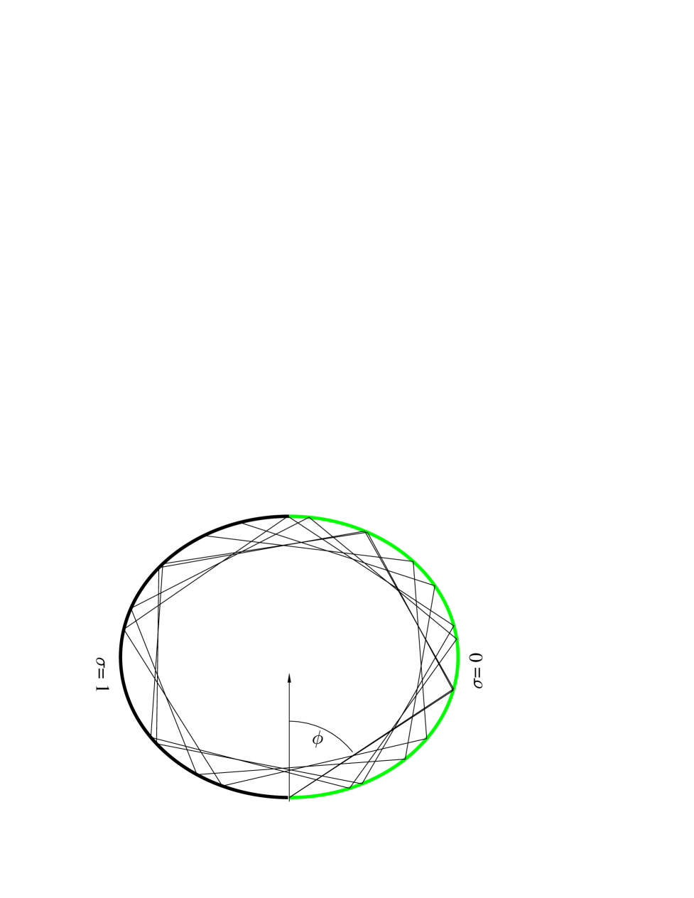
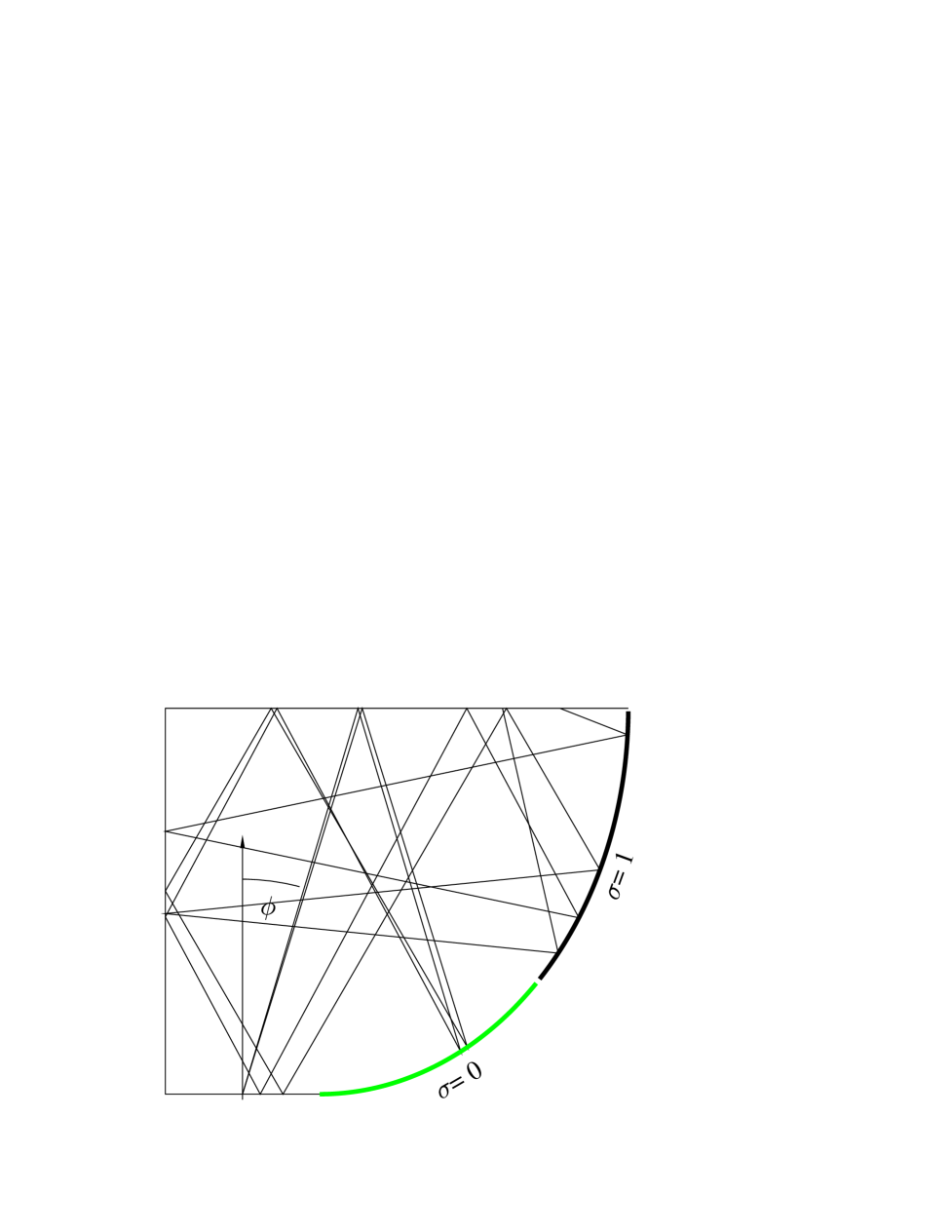
The billiard in a circle (Fig. 1) is a noticeable example of Liouville-Arnol’d (L-A) integrability: the second, smooth integral of the motion being the angular momentum with respect to the center. Cutting the circle in two equal pieces, and inserting a rectangular strip in between the two halves gives rise to a fully chaotic billiard: the stadium [20]. We shall get rid of all symmetries in this geometrical figure, and study the quarter stadium (Fig. 2). Let us now replace the circular sides in both billiards by a polygonal approximation with equal sides: it is apparent that this can be done so to form a rational billiard. In both these cases, Vega, Uzer and Ford have found exponentially divergent trajectories, within their approximation scheme of course. In the following, I shall show that the two cases are different indeed. To do this, I first need to introduce a symbolic coding of this problem.
How to code a dynamical object into a symbolic sequence is something which follows either from physical insight, or practical convenience, or mathematical efficacy. In our case, we shall elect to code trajectories according to the bounce coordinate alone: for this, we shall assume that the circular parts of the boundary (or their polygonal approximations) are divided into a finite number, , of equal regions, each of which corresponds to a symbol, , which can be taken to be a natural number from to . We also decide that bounces on the straight segments of the stadium will not be registered. This coding is indicated in Figures 1 and 2, for . In a billiard game like this, we may think of putting detectors all around the boundaries, which are set off whenever the ball hits them. In the polygons, nearby sides can be connected to the same detector, so that the total number of output channels is , also when –the number of sides–is much larger than , and is allowed to increase, while keeping fixed, as we shall do in the following. The history of a trajectory is then coded in the record of boundary reflections.
Now, let us play a funny game: the ball is initially set still at a fixed point, and a test player–chosen appropriately among our pals–can aim it by hitting it properly by the conventional cue. As the departing angle is varied different trajectories are initiated, and different symbolic sequences are recorded. Let us now ask the player to do it twice, that is, to aim the ball a second time so that the sequence of bounces he had obtained in the first shot is repeated [21]. It comes as no surprise that he will not be able to set the initial angle to exactly the same value in both tries: the difference in this quantities causes the two resulting symbolic trajectories to agree only over a finite time-span. Trajectories of this kind are pictured in Figures 1 and 2. But how is this sport related to algorithmic complexity and to our problem ?
IV Deterministic Randomness of Finite Trajectories
In the light of the previous section, a billiard can be thought of as a computer program, that is, a Turing machine capable of taking a binary sequence –the program, to which we shall momentarily return–as input, and producing a symbolic sequence, , the output. Recall now that the algorithmic complexity of a sequence , for is defined very roughly as the length of the shortest computer program capable of outputting the sequence, and stopping afterwards [22, 23]. We can say that the complexity of a sequence is the length of its shortest definition:
| (2) |
Algorithmic complexity theory teaches us that most sequences–in probabilistic sense–of length have complexity close to maximal, i.e. . Moreover, in the limit of increasing , almost all of them are random, in the sense that their complexity grows as [24]. At the same time, computable sequences exist, for which is much less than , and grows less than linearly. We apply now this theory to the dynamical sequences constructed in the previous section. Let us call their complexity , where we have explicitly indicated that this number may depend on the initial condition of the motion. We shall then follow Alekseev [15], Chirikov [25], and Ford [26], and identify order with computability, and chaos with randomness.
The central issue is then to find a computer code to output the desired sequence. For our dynamical sequences, , this can be obtained in any abstract language by an encoding of: a) the geometrical rules of the game, which require a fixed number of bits, (which depends only on the machine on which the rules are coded), plus b) the instructions set for fixing the billiard boundaries, of length , plus c) the specification of and d) of a certain number of digits of . Accordingly, the length of this program can be estimated as
| (3) |
where the function is defined as the number of bits of necessary and sufficient to determine the first symbols in the sequence . This function can serve to estimate the complexity in its most important aspect: the dependence. For it is clear that the opposed behaviors presented above–random and computable–are of deep physical significance: if in a range the function grows linearly, the complexity has the same leading behaviour, and the sequence should duly be termed random, or chaotic. When, in a similar interval, grows less than linearly, should be called computable, or ordered. We therefore introduce the notion of order (and randomness) within a range. The physical significance of such order (or randomness) will then be proportional to the importance of such range.
We have emphasized this scaling approach in [3] to rebut a common objection to the application of complexity theory to finite dynamical sequences [27]. The rationale behind this idea is evident, and is quite similar to that adopted in the independent theory of computational time complexity: not so much the value of complexity is relevant, but the way it increases as the problem size grows, for this may render it quickly unfeasible. In fact, there is no point in practicing for our billiard player if he is playing a chaotic billiard: for each additional bounce he wants to set correctly his aiming precision in the initial angle must increase geometrically. Out of metaphor, when the billiard is a system whose symbolic dynamics we want to predict, to obtain a linear increase in forecast precision we must exponentially increase the accuracy in the initial conditions [28]. In most instances this demands an exponential increase of economical resources.
V The Circle and the Stadium–Polygonal Quantization
To draw a parallel with quantum mechanics [29] suppose now that Nature, by means of our observations, clearly shows that curved billiard boundaries are a mathematical idealization and that physically we can just have polygonal billiards with an arbitrary but finite number of sides, . These sides will be inscribed in the circle and in the stadium, and I shall call the resulting polygonal billiards a quantization of the curved ones. In this context, is a crucial quantity, which plays the rôle of a semi-classical parameter. Clearly, when we let go to infinity we regain geometrically the original table. The question is, will we obtain the same dynamics ?
To answer this question in a complete, algorithmic sense, let us consider again the coding introduced in Sect. III, and let us study the function defined in Sect. IV, or rather its inverse, , which quantifies the number of symbols which can be predicted knowing digits of . It is clear that order (or randomness) of a dynamical sequence can also be inferred from the study of . Moreover, this function has a transparent physical meaning: if we let , in this new independent variable the function can be called the length of the codable trajectory under uncertainty . Let us go back to the player example. He is only capable of setting the angle with a certain error . Under these circumstances, only finitely many dynamical symbols will typically coincide in the initial portions of a series of two shots and : their number is ,
| (4) |
Following [30] we also say that is the first error time, when any two initially -close trajectories start to have different symbolic sequences.
Numerically this function is rather straightforward to compute, and its theoretical analysis can be carried out in full detail (see the Appendix and below). It is plotted in Fig. 3 versus at fixed uncertainty , for the quantization of the circle (a regular octagonal billiard). One observes that low values, like that seen at , are associated with trajectories heading very early in history towards a vertex, where a symbolic error may occur [30, 6]. Large values of are found when this happens much later: is associated with a periodic trajectory which stays far away from the vertices [31].
It can be shown that the behaviour of at the periodicity values is at the root of the dynamical properties of the system. In fact, let the ideal, frictionless ball run for an infinite time. A coding function of the initial angle can be defined as
| (5) |
This function represents the translation dictionary between the trivial code–the infinite sequence of digits of , and the dynamical code–the infinite sequences of bounces. In chaotic systems, like the motion over surfaces of constant negative curvature, and the anisotropic Kepler problem, the relation between the properties of and the function can be fully exposed. This relation justifies the multi-fractal properties of the coding function , which were originally investigated by Gutzwiller and Mandelbrot [32, 33].

In player’s terms, the angle in Fig. 3 is an easy shot, and a tough one: we find then convenient to average over initial angles, so defining the average coding length :
| (6) |
which will become our main indicator of the complexity of the motion. A canonical average over the full phase space can be also defined and computed, with quantitatively similar results to those we are going to expose. Let us pause no more, and compare the behavior of this quantity in the circle, the stadium, and their polygonal quantizations.
VI Orbital complexity in integrable and polygonal billiards
We have now set the stage for the examination of the average orbital complexity in our billiards. We start from the case of the circle and its polygonal approximations: before resorting to exact analysis, let us have a look at the numerical data. Fig. 4 plots versus . The scale is doubly logarithmic: according to eq. (3) the power-law behavior of these curves for small is a manifestation of the ordered character of the motion, which is well assessed in the literature [8], [15], [6].

Yet, the physical picture evident in Fig. 4 is much richer. Firstly, as grows at fixed (large) , tends to , where the label is self-explanatory, the earlier the larger the value of . This is indeed clear: at large the coding length is short, and differences between polygonal boundaries with large and the circle are not significant. But if we turn now our attention to the left part of Fig. 4, where relatively smaller values of are plotted, a less expected phenomenon appears: increasing at fixed the difference between and seems to grow rather than vanish. Moreover, this discrepancy is brought about by a decreasing . Recall that is the average of the inverse function of (if you rotate the graph clockwise by ninety degrees, appears plotted on the horizontal axis and on the vertical): in this region the complexity of a trajectory of fixed length grows when is increased. This is the phenomenon observed by Vega, Uzer and Ford: polygonal billiards have their own brand of instability, generated by splitting of trajectories at vertices. The more the vertices, the larger the Lyapunov numbers computed in [11]. The paradox presented in Sect. II is so exposed.
But we are now equipped to resolve it: observe first that the increase in complexity obtained by raising at fixed is only temporary: if we keep going, we find that finds a minimum, and then inverts its course to reach quickly (we shall come back on the rate of this convergence later on) the circle value [34]. Furthermore, a deeper argument must be made: sitting at fixed is not a proper thing to do, not even in the presence of human limitations to finite precision. In fact, we cannot increase precision indefinitely, but we certainly can over a finite, physically reasonable range. For instance, this may be dictated by the computational power of the machine on which Fig. 4 has been computed. Exploring this range, from larger to smaller uncertainties, we discover that starts off like the L-A-integrable circle, , and successively redirects its course on a different line, with the same exponent: a transition from L-A to A-integrability has taken place.
These observations can be derived rigorously from the analysis developed in the Appendix, with the result:
| (7) |
where the crucial functional dependence on is apparent, and where is a constant, which plays a similar rôle to Planck’s constant in the “usual” quantum mechanics. In the above equation, the first behaviour is that of the pure circle (correspondence). The second equation in (7) leads to an estimate for the average complexity which increases only logarithmically with and :
| (8) |
where is a positive constant, independent of and , and therefore from eq. (3) one obtains [35]
| (9) |
where is another positive constant. This result should be compared with the existing literature on the topological complexity of symbolic dynamics [36].
In conclusion, we see that vertices add logarithmically to the complexity, but only as long as , i.e. . We have so reconciled the observation of ref. [11] and the established knowledge on polygonal billiards. We can now turn to a more delicate problem: what happens of orbital complexity in the polygonal approximations of a chaotic billiard.
VII Orbital Complexity and Correspondence in Chaotic Billiards
In the previous section we have established that rational approximations of the circle cannot be called chaotic, not even under the assumption of finite precision. Is this achievement possible to their more sophisticated relatives, those inscribed in the stadium ? After all, as tends to infinity, these fellows tend to a fully chaotic system, and one thing is certain, correspondence principle must be obeyed [39].

Fig. 5 is the analogue of Fig. 4, now for the quarter stadium billiard table. The abscissa is in log scale, i.e. minus . The logarithmic character of the curve clearly reveals that the complexity of trajectories grows linearly with length: chaos is here manifest in its essence. For large values of , is roughly equal to . For instance, over the interval is a logarithmic function of ; we can therefore expect that a corresponding range in exist so that the average complexity grows linearly: here, trajectories are random, in the sense explained in Sect. IV. Notice that the existence of this range is what permits “sensible” numerical experiments of chaotic motion.
The effect of vertices noticed in the circle quantization appears again when following the curve to the left, as it leaves staying slightly lower than this latter, i.e. showing a relative increase in the complexity of the motion. As noted above, this increase is quantified by the logarithmic contribution . Alas, this excess of zeal rapidly turns into failure: the algorithmic simplicity of polygonal boundaries is soon detected, and starts to grow like . What has happened is that the complexity estimate (8), previously dominated by that of the curved stadium, takes over for good. In fact, an exact analysis can be performed here too, showing that
| (10) |
where , , and are suitable constants, the last playing the same rôle as in the previous section. Consequently to this equation, in the region complexity estimates of the form (8), (9) still apply.
The end of this paper is in sight, and we must start drawing conclusions. There is a significant difference between the case of the circle (Fig. 4 and eq. (7) ) and of the stadium quantization (Fig. 5 and eq. (10)): while the former, as we noted, shows a transition from A to L-A-integrability, the second matches A-integrability with randomness, and this mating is troublesome, to say the least. Perhaps the most evident consequence is the following: let me ask how long must a symbolic sequence be to perceive the finiteness of the number of boundary sides via its algorithmic manifestations. The answer is instructive. In the polygonal quantization of the circle, and of the stadium as well, the critical value at which the curve is abandoned scales as . Yet, at the same time the different structures of the two problems imply that the length of polygonal-curved accordance is proportional to in the integrable case, and only to the logarithm of for the chaotic stadium [40].
These results have been obtained by explicit calculation. Yet, I believe their algorithmic nature to be more important: we must realize that both circle and stadium polygonal quantizations are dynamical systems endowed with an amount of complexity which scales as the logarithm of . Yet, while the -circle dynamics unfolds this complexity slowly, at a logarithmic pace, its -stadium relative does it eagerly, linearly in time, so that the complexity reservoir is quickly exhausted. In the Conclusions I shall briefly present my views on the physical implications of these facts.
VIII Conclusions: Chaos in Nature, is There Any ?
Algorithmic complexity theory, used here in a physicist’s fashion via the concept of average first error time, clarifies the simplicity of the dynamics of polygonal billiards, and offers a solution of the paradox which arises from the juxtaposition of ref. [6] and [11]. At the same time, this theory provides a complete characterization, in all ranges of parameters, of the dynamical properties of the families of billiards studied in this paper. These latter, in turn, are significative representatives of integrable and chaotic billiards, and we can safely expect our results to be quite general.
In essence, the algorithmic estimates derived in this paper are manifestations of the same phenomenon observed in the Schrödinger quantization of the Arnol’d cat [43, 2, 3, 5] (see eqs. (8) and (9) of ref. [3]), of bounded systems [4], and in the classical dynamics of discrete systems (see Sect IV of ref. [30]). Truly then, the nature of chaos and order is information content ! Yet, if we admit this, we must be prepared to bear the consequences when going back to the problem of quantum mechanics: then, the metaphor of rational billiards exposed here permits to understand the claim that the correspondence principle is validated for integrable systems, and violated for chaotic ones. It was shown in the last section, in fact, that in the first case a discrete nature–in which only polygons are allowed–would let us play with our curved theoretical models for a long time. For the same reason, in the quantum mechanics of an integrable system, the action of increasing a semi-classical parameter provides a complexity reservoir which keeps up with the classical description for a time-span which grows appreciably, as a power-law, in this parameter. In the second case, to the contrary, the time of chaotic freedom is logarithmically short, and the essence of correspondence, to regain classical/curved complexity by quantum/polygonal computations is exponentially remote in the semi-classical parameter [41]. Quantum dynamics is a computable theory, and can “correspond” to the uncomputable classical mechanics only as far as its algorithmically simple nature allows it [42].
Notwithstanding this evidence, people have been for a long time reluctant to admit that there is not such a thing as “quantum chaos”, or that this chaos is something different–and less–than deterministic randomness. This hindrance is now history. To the contrary, Boris Chirikov has appreciated this fact since the very beginning, and his notions of transient chaos [25] and pseudo-chaos [44], [45], show this very clearly. Moreover, he has put a strong emphasis on this latter concept: largely simplifying, but I believe appropriately, one could say that Chirikov views the pseudo-chaos (that we call A-integrability) of discrete systems (and by consequence of the digital computers as well) as a faithful representation of what takes place in quantum mechanics [46]–and in nature, at all levels. At this very last point we part company: in fact, an unsettled debate still holds on the meaning and validity of the correspondence principle [47], and on the question whether quantum A-integrability is enough to cope with a world in which chaos seems to be essential. In my works with Joe Ford a negative answer to this question has been presented, suggesting that–in this sense–quantum mechanics might be incomplete, and that the “reductionist” program of deriving classical chaos from quantum mechanics could not be achieved [48].
Certainly, classical mechanics is inadequate to describe reality, but it contains the gene of non-computability, which we believe should be present in a complete theory of nature; at the same time, the more fundamental quantum mechanics inherited this gene in too a tame form to be effective. This is, in nuce, the point of contention. Will time settle the matter–or will it be that the general indeterminacy principle foreseen by Ford [49] will change everything around ?
IX APPENDIX: Average first error time calculation
We shall now justify the formulae presented in Sects. VI and VII via a direct calculation of the average first error time . Firstly, let us consider the case of the (integrable) circular billiard. The angle is a constant of the motion: letting the motion is , the usual ergodic (for irrational ) rotation of the circle. Trajectories with different initial angle separate at a linear speed , where has the same meaning as in the main body of the paper (see Fig. 1). Consequently, a bunch of trajectories opens up linearly in time like a slightly unfocused light beam. An error occurs when a boundary point of the circle partition which determines the coding enters this light cone. Let us now estimate the average time required for this to happen.
Let to be the number of cells of the partition of the boundary, and their common length. Let also , . According what we have just said, an error occurs when the angle of the reference trajectory (the center of the beam) comes within of zero or one, where . Let be the probability that the first error occurs at time . Ergodicity implies that . Certain approximations are required to evaluate for : we assume that , are uncorrelated random variables, so that . Estimating then the asymptotic (small ) behaviour of by standard techniques gives and therefore
| (11) |
which well reproduces the behaviour numerically found in Sect. VI.
Surprisingly, the same dependence can be shown to hold for the polygonal billiards considered in this paper. The presence of the vertices imposes a more sophisticated analysis. When the beam bounces fully on the same polygonal side, its angular amplitude is conserved, and its transverse dimension grows linearly in time on average, exactly as it does in the circular billiard. To the contrary, when the beam impinges on a vertex of amplitude , its angular amplitude is increased by the amount . In the polygonal approximations of the circle, we have , while for the quarter stadium, so that is the resulting perturbation in the circular case, and in the quarter stadium.
Two regimes must now be considered. Firstly, when is much larger than , the effect of vertices is negligible, trajectories behave as in the corresponding curved billiards, and coincides to a good approximation with . In the opposite regime, when is much larger than , impinging on a vertex causes a major enlargement of the beam. We can assume that this leads almost immediately to an error: a similar analysis to that performed in the circular case can then be carried out. We let be the approximate length of the polygonal sides: this quantity plays here the same rôle did above. The result is then
| (12) |
for the -circle, and
| (13) |
for the -stadium, where is a parameter which measures the effective length of trajectories in between two coded bounces. Finally, the intermediate region between the two regimes is determined by the condition described above, which becomes the “indeterminacy principle” , where is a constant.
REFERENCES
- [1] Correspondence Principle states that classical mechanics gives the right (i.e. quantum) results when the action per cycle is large compared to Planck’s constant (P.A.M. Dirac, The Principles of Quantum Mechanics, Oxford 1947).
- [2] J. Ford, G. Mantica, and G. Ristow, Physica D 50 (1991) 493-520.
- [3] G. Mantica and J. Ford, in Quantum Chaos–Quantum Measurement, P. Cvitanović, I. Percival, and S. Wirzba Eds, (Kluwer, Dordrecht, 1992).
- [4] J. Ford and M. Ilg, Phys. Rev. A 45 (1992) 6165-6173.
- [5] J. Ford, and G. Mantica, Am. J. Phys. 60 (1992) 1086-1098.
- [6] B. Echardt, J. Ford, and F. Vivaldi, Physica D 13 (1984) 339.
- [7] A.N. Zemlyakov and A.B. Katok, Math. Notes 18 (1976) 760; Math. Notes 20 (1976) 1051.
- [8] Ya.G. Sinai, Introduction to Ergodic Theory, (Princeton Univ. Press, Princeton, 1976).
- [9] E. Gutkin, Billiards in Polygons, Physica D 19 (1986) 311-33, and Billiards in Polygons: Survey of Recent Results, J. Stat. Phys. 83 7 (1996).
- [10] P.J. Richens, and M.V. Berry, Physica D 2 (1981) 495.
- [11] J.L. Vega, T. Uzer, and J. Ford, Phys. Rev. E 48 (1993) 3414.
- [12] G. Gallavotti, and D. Ornstein, Comm. Math. Phys. 38 (1974) 83-101.
- [13] D. Ornstein, Science 246 (1989) 182-186. D. Ornstein and B. Weiss, Bull. Am. Math. Soc. 24 (1991) 11-116.
- [14] J. Ford, in Long Time Predictions in Dynamics, C.W. Horton, L.E. Reichl, and V.G. Szebehely, eds. (Wiley, N. York, 1983) 79.
- [15] V. M. Alekseev, and M.V. Yakobson, Phys. Repts. 75 (1981) 287.
- [16] For a general introduction to complexity and dynamics, see R. Badii and A. Politi Complexity, Hierarchical Structures and Scaling in Physics, (Cambridge University Press 1996).
- [17] I follow here Echardt’s et al. appreciation in ref. [6].
- [18] These errors which take place at vertices in polygonal billiards have been studied e.g. in A. Hobson, J.Math. Phys. 16 (1975), 2210-2214, G. Casati and J. Ford, J. Comp. Phys. 20 (1976) 97-109, and F. Henyey and N. Pomphrey, Physica D 6 (1982) 78.
- [19] P.J. Richens, and M.V. Berry, in [10] call these systems pseudo-integrable.
- [20] L.A. Bunimovich, Comm. Math. Phys. 65 (1979) 295-312.
- [21] This game is not as uncommon as it might seem: who has not been challenged, after a good shot, to do it again if you can ?
- [22] A.N. Kolmogorov, Probl. Peredachi Inform. 1 (1965) 3-11.
- [23] G. Chaitin, Information, Randomness, and Incompleteness, (World Scientific, Singapore, 1987).
- [24] Although logarithmic corrections may be present: , they are clearly subdominant w.r.t. the leading linear behaviour, see P.M. Löf, J. Inf. Control 9 (1966) 602-619.
- [25] B.V. Chirikov, F.M. Izrailev, and D.L. Shepelyansky, Sov. Sci. Rev. C2 (1981) 209.
- [26] J. Ford, Phys. Today 36, (1983) 40-48.
- [27] It is frequently claimed that chaos, especially when intended as deterministic randomness is only definable in the infinite time limit. For finite sequences the indeterminacy due to the necessary recourse to a universal computer would prevent us to make clear-cut distinction between ordered and random sequences, and–it is then pretended–no no statements about order or chaoticity of a finite-time evolution could be substantiated. Counting the number of sequences of length with complexity less than , (see e.g. [5]) provides a first answer to this objection. The scaling answer adopted in this paper was presented in [3], and applied to the definition of chaos in systems with a finite number of states–where similar problems arise–in [30].
- [28] This hints at the relation between complexity and Lyapunov exponents: see A. Brudno, Russ. Math. Surv. 33 (1978) 197, and P.R. Baldwin, J. Phys. A: Math. and Gen. 24 (1991) L941-L947, which also describes a coding procedure for the Sinai billiard.
- [29] For a discussion of the proper quantum mechanical correspondence, see L.A. Ballentine, Quantum Mechanics, (Prentice Hall, Englewood Cliffs, N.J. 1990). L. A. Ballentine has compared quantum dynamics with the classical dynamics of Liouville distributions: Phys. Rev. A 47 (1993) 2592-2600, Phys. Rev. A 50 (1994) 2854-2859, Phys. Rev. A 54 (1996) 3813-3819.
- [30] A. Crisanti, M. Falcioni, G. Mantica, and A. Vulpiani, Phys. Rev. E 50 (1994) 1959-1967. In this paper, the algorithmic similarity between Hamiltonian systems in discrete phase space and quantum mechanics is exhibited.
- [31] The periodic orbit theory of this function is interesting, but will not be developed in this paper.
- [32] M.C. Gutzwiller and B.B. Mandelbrot, Phys. Rev. Lett. 60 (1988) 673. M.C. Gutzwiller, Physica D 38, (1989) 160-171.
- [33] D. Bessis and G. Mantica, Phys. Rev. Lett. 66 (1991) 2939.
- [34] The same result was within reach of Vega et al. [11], had they continued their circle calculations, Fig. 10, beyond their “saturation” value.
- [35] When computing from , observe that the coding length of the set of boundaries can be easily shown to be logarithmically increasing in .
- [36] Establishing rigorous bounds on the algorithmic complexity of orbits in billiards is an important and difficult enterprise. Yet, rigorous analysis cannot, at the moment, catch most of the phenomena outlined in this paper. Consider, for instance, the topological complexity of a symbolic dynamics, which is defined as the number of words of length less than, or equal to , and is denoted by [9]. Controlling this number can give a bound on the algorithmic complexity of any orbit, via a lexicographic argument: does not exceed a constant plus . For rational billiards, perhaps the best available result [37] is , see also [38]. It must be observed that in this paper we group different sides in the same letter, and we do not code certain rebounds (in the stadium, see text). This situation differs from that in which the estimate above has been derived. Yet, in adapting these estimates to the -circle, one would get , which is to be compared with the result following from eq. (9), which involves an average, in the sense explained in this paper. It appears that while our result agrees with the lexicographical estimate, this latter bears no evidence of the number of sides of the polygon, and the related analysis has significance only in the asymptotic region of vanishingly small .
- [37] P. Hubert, Complexité de suites définies par des trajectoires de billiard, Thèse, Institut de Mathématiques de Luminy, Univ. Marseille, France, 1995.
- [38] S. Troubetzkoy, Chaos 8 (1998) 242.
- [39] Capitalized statement of a colleague that Joe Ford had provocatively posted on a wall in his office.
- [40] This algorithmic fact gives reason of the so-called Zaslavsky time-scale in chaotic systems, , where is the action, and the maximum Lyapunov exponent: G.P. Berman and G.M. Zaslavsky, Physica A 91 (1978) 450, G.M. Zaslavsky, Phys. Rep. 80 (1981) 157-250.
- [41] Conversely, just because its algorithmic content is low, quantum dynamics of chaotic systems can be computed efficiently (for times larger than the Zaslavsky time-scale) by semi-classical algorithms: S. Tomsovic and E.J. Heller, Phys. Rev. E 47 (1993) 282-299. It is interesting to read this paper on the quantum stadium in the informational-theoretical setting of algorithmic complexity proposed here, and to compare it with K.M. Christoffel and P. Brumer Phys. Rev. A, 33 (1986) 1309-1321, also on the stadium billiard. Of course, this comparison must also include ref. [4], which studies in full generality the complexity of the motion in bounded quantum systems and shows its computability.
- [42] We have focused attention here on trajectories: when going back to the proper quantum-classical correspondence recall that it should be discussed in terms of many-to-many relations (like e.g. many classical trajectories to a set of quantum eigenstates) [2, 3].
- [43] J.H. Hannay, and M.V. Berry, Physica D1 (1980) 267.
- [44] B.V. Chirikov, in Chaos and Quantum Physics, M.-J. Giannoni, A. Voros, and J. Zinn-Justin Eds., (Elsevier, Amsterdam 1991).
- [45] Following Ford, I do not favour the term pseudo-chaos, for historical [7, 14] and linguistic reasons make A-integrability preferrable: pseudo-chaos, and quantum chaology [48] as well, are negative definitions, in the sense that they hint to something less, or other than chaos; A-integrability, to the contrary, positively says what replaces the simple Liouville-Arnol’d notion of integrability. On a side, it is interesting to remark that the term pseudo-integrability [10] has also been proposed to denote the motion in rational billiards. The funny note here is that the same dynamics is pseudo-integrable to some authors, and pseudo-chaotic to some others.
- [46] For an introduction to the physical aspects of the so-called quantum chaos, see M.C. Gutzwiller, Chaos in Classical and Quantum Systems, (Springer Verlag, Berlin 1980), and B.V. Chirikov and G. Casati, Quantum Chaos, (Cambridge Univ. Press, 1995).
- [47] R.V. Jensen, Nature 355 (1992) 311.
- [48] It is interesting to consider comparatively the interpretation of M.V. Berry, in Chaos and Quantum Physics, M.-J. Giannoni, A. Voros, and J. Zinn-Justin Eds., (Elsevier, Amsterdam 1991). Also notice that we never consider quantum systems open to external perturbations of stochastic nature, as e. g. in R. Schack and C. M. Caves Phys. Rev. E 53 (1996) 3257-3270.
- [49] J. Ford, in The New Physics, P.C.W. Davies Ed. (Cambridge Univ. Press, 1989).