Escape Orbits and Ergodicity in Infinite Step Billiards

Abstract

In [DDL] we defined a class of non-compact polygonal billiards, the infinite step billiards: to a given sequence of non-negative numbers $\{p_{n}\}_{n\in{\mathbb{N}}}$, such that $p_{n}\searrow 0$, there corresponds a table $P:=\bigcup_{n\in{\mathbb{N}}}[n,n+1]\times[0,p_{n}]$.

In this article, first we generalize the main result of [DDL] to a wider class of examples. That is, a.s. there is a unique escape orbit which belongs to the $\alpha$- and $\omega$-limit of every other trajectory. Then, following the recent work of Troubetzkoy [Tr], we prove that generically these systems are ergodic for almost all initial velocities, and the entropy with respect to a wide class of ergodic measures is zero.

AMS classification scheme number: 58F11

1 Introduction

Playing on a rectangular billiard with just one ball can be a boring experience, in particular when the ball is represented by a point: given any starting position, the corresponding orbit is dense on the billiard for almost all directions, whereas for a countable set of initial angles all orbits are periodic.

We can make the game a little more interesting if we use a generic polygonal billiard.

Remark 1

In more generality, billiards are dynamical systems defined by the uniform motion of a point inside a piecewise-differentiable planar domain (the table), with elastic reflections at the boundary. This means that the tangential component of the velocity remains constant and the normal component changes sign [T].

A polygonal table is called rational when the angles between the sides are all of the form $\pi n_{i}/m_{i}$, where $n_{i}$ and $m_{i}$ are integers. These billiards have the nice property that any orbit will have only a finite number of different angles of reflection $\vartheta$. In this case, there is a natural unfolding procedure [FK, KZ] which allows one to map any given trajectory on the table to an orbit of a vector field over a surface having a certain genus.

Remark 2

Usually one assumes that the magnitude of the particle’s velocity equals one, and that the orbit which hits a vertex stops there. For our model, though, we will slightly modify this second assumption, since it is possible to continue uniquely every trajectory for all values of $t$ (see later). Either way, the set of initial conditions whose orbits do not contain any vertices is always a set of full measure in the phase space.

The aforementioned rational condition implies in particular a decomposition of the phase space in a family of flow-invariant surfaces $S(\vartheta),\ 0\leq\vartheta\leq\pi/m,\ m:=l.c.m.\{m_{i}\}$. Excluding the special cases $\vartheta=0,\pi/m$, it is known that the billiard flow restricted to any of the $S(\vartheta)$ is essentially equivalent to a geodesic flow $\phi_{\vartheta,t}$ on a closed oriented surface $S$, endowed with a flat Riemannian metric with conical singularities [G3].

Based on this fundamental idea, many important and deep results have been proven, with the crucial aid of some highly non-trivial mathematical techniques. In particular, the theory of quadratic differentials over Riemann surfaces, the theory of interval exchange transformations (using the induced map on the boundary) and the method of approximating irrational billiards with rational ones, have altogether turned out to be very effective to understand the dynamics of polygonal billiards. References [G2, G3] give a complete account of the state-of-the-art in this field, and [DDL], of which this paper is a follow-up, contains a compact reference list.

Here we limit ourselves to recall only those results that will be of immediate use in the rest of the paper:

• [KMS, Ar, KZ] The Lebesgue measure in a (finite) rational polygon is the unique ergodic measure for the billiard flow, for (Lebesgue-)almost all directions. Moreover, for all but countably many directions, a rational polygonal billiard is minimal (i.e., all infinite semi-orbits are dense). In particular, for almost integrable billiards, “minimal directions” and “ergodic directions” coincide [G1, G2, B]. (Roughly, an almost integrable billiard is a billiard whose table is a finite connected union of pieces belonging to a tiling of the plane by reflection, e.g, a rectangular tiling, or a tiling by equilateral triangles, etc.—see [G2, G3] for more precise statements.)

• [KMS] For every $n$, in the space of $n$-gons there is a dense $G_{\delta}$-subset of ergodic tables.

• [G3, GKT] For any given polygon, the metric entropy with respect to any flow-invariant measure is zero. Furthermore, the topological entropy is also zero.

• [GKT] Given an arbitrary polygon and an orbit, either the orbit is periodic or its closure contains at least one vertex.

All of these results, however, fail to hold when we introduce further complications: an infinite number of sides (an interesting example is the “staircase” compact billiard briefly mentioned in [EFV], while the inspiring paper by Troubetzkoy [Tr] discusses the general case), or non-compact tables (one might take a look at [GU, Le], although they are not about flat polygonal billiards).

In [DDL] we introduced a family of (seemingly) simple models that have both properties: the infinite step billiards (Fig. 1).

Figure 1: An infinite step billiard.

For them, it turns out that one of the first non-obvious questions to treat is exactly what our friend that likes playing pool more than handling groups of automorphisms would like to know: depending on how I initially hit the ball, can I be sure it will come back at all? In other words, since the system is open it makes sense to ask how many orbits actually keep returning to the “bulk” of the systems rather than escaping. As a matter of fact this was one of our main motivations in [DDL]. In the one example we treated in detail there, we found that the fact that there is a unique escape orbit for a.a. directions has very interesting implications for the dynamics of the entire billiard: specifically, this orbit is somehow an “attractor” for the system. We will re-state this more precisely in Section 2.1.

Here we consider the whole class of infinite step billiards and we will see that playing on these tables can be rather challenging, even if we pay the price that sometimes we have to wait a little bit before our ball comes back. It turns out that the above result on the uniqueness of the escape orbit can be extended—together with its corollaries—to a wide set of billiards in our class. For these tables, the typical situation is that the ball keeps returning to the leftmost wall, although each time it might stretch arbitrarily far to the right, following the unique, ill-behaved, escaping trajectory. This is basically what Theorem 1 and related statements assert—see in particular Proposition 2. (Incidentally, we are pleased to attest that further work in this direction is in progress [Tr2].)

More theoretically, one would like to know better about the ergodic properties of these systems (at least of many of them).

Recently Troubetzkoy [Tr] treated the case of an arbitrary polygon with an infinite number of sides, proving interesting results regarding both the topological structure (e.g., Poincaré Recurrence Theorem and existence of periodic trajectories) and the ergodicity. In particular, he showed that the typical bounded infinite polygon has ergodic directional flows for almost all angles. The notion of typicality as first used by [KZ] is now customary (see also [KMS]): in a certain topological (usually metric) space there exists a dense $G_{\delta}$-set of billiards with that property. The metric used in [Tr] requires several conditions to be verified before two polygons can be considered close: their shapes are to be very similar, of course, but also the two flows are to keep close for a long time, for many initial conditions. (Not that one could do much better. In fact, it is not hard to imagine two infinite polygons that look alike but have completely different dynamics—which is exactly the point in [EFV] when the staircase model is presented.)

The other results in this paper apply the ideas of [Tr]. We show that generic ergodicity holds for the family of unbounded, finite-volume, billiards in our class (Theorem 3). The metric we employ, however, is very simple and can be expressed in terms of “easily measurable” quantities. Also, we prove that the entropy of the billiard is zero w.r.t. any invariant ergodic measure that verifies a cartain finiteness condition (Proposition 4).

The topological entropy, too, is probably zero (at least for many of these systems) but, due to the non-compactness of the table, the usual variational principle cannot be applied directly and one must check some additional conditions [PP].

In the next section we introduce the basic notation (referring the reader to [DDL] for a more detailed presentation of the systems in question), we give some quick proofs, and we present the precise statements of our results. The main proofs are then distributed in the following sections.

Acknowledgments: We would like to thank L. Bunimovich and S. Troubetzkoy for stimulating discussions. M. D.E. contributed to this paper during his visit to the School of Mathematics of the Georgia Institute of Technology, whose support and excellent working conditions he gratefully acknowledges.

2 Notations and Statements of the Results

In this paper we are interested in a class of rational billiards, the infinite step billiards, defined as follows: Let $\{p_{n}\}_{n\in{\mathbb{N}}}$ be a monotonically vanishing sequence of non-negative numbers, with $p_{0}=1$ (we will later relax this inessential last condition). We denote $P:=\bigcup_{n\in{\mathbb{N}}}[n,n+1]\times[0,p_{n}]$ (Fig. 1) and we call $(x,y)$ the two coordinates on it.

A point particle can travel within $P$ only in four directions (two if the motion is vertical or horizontal—cases which we disregard). One of these directions lies in the first quadrant. For $\vartheta\in]0,\pi/2[$, the invariant surface associated to the billiard flow is labeled by $S^{P}(\vartheta)$ (or just by $S(\vartheta)$, when there is no means of confusion). This manifold is built via the usual unfolding procedure with four copies of $P$. We denote by $(X,Y)$ the intrinsic coordinates on $S^{P}(\vartheta)$, inherited by its represention on a plane $(x,y)$, with the proper side identification (see Fig. 2). The $3\pi/2$ corners represent the non-removable singularities, or singular vertices, $V_{k}$, of coordinates $(k,p_{k})$ on $P$, or $(\pm k,\pm p_{k})$ on $S$.

Figure 2: The invariant surface $S^{P}(\vartheta)$ for the infinite billiard.

With the additional condition $\sum_{n}p_{n}<\infty$, $S^{P}(\vartheta)$ can be considered a non-compact, finite-area surface of infinite genus.

Remark 3

In [DDL] we used $R_{\alpha}$ to denote the invariant surface for a given $\alpha=\tan\vartheta$. More importantly, we measured the directions w.r.t. the Lebesgue measure for $\alpha\in]0,+\infty[$. However, this is equivalent to the normalized Lebesgue measure for $\vartheta\in]0,\pi/2[$. In this paper we use angles except in Section 3, where it is convenient to do otherwise.

We will denote by $P^{(n)}$ the truncated billiard that one obtains by closing the table at $x=n$. The corresponding invariant surface, of genus $n$, will be denoted by $S^{(n)}(\vartheta)$ (Fig. 3). Some statements about $P^{(n)}$ have immediate consequences for the infinite table $P$. For instance:

Figure 3: The invariant surface $S^{(n)}(\vartheta)$ for the truncated billiard.

Proposition 1

In an infinite step billiard $P$, for almost all $\vartheta$, all semi-orbits are unbounded, whereas periodic and unbounded trajectories can coexist for a zero-measure set of directions.

Proof. (See also [DDL], Proposition 4.) For any given $\vartheta$ and $n>1$, we denote by $\phi_{\vartheta,t}^{(n)}$ the flow on $S^{P^{(n)}}(\vartheta)$. Let

$${\cal M}_{n}:=\{\vartheta\in]0,2\pi[\>\big{|}\>\phi_{\vartheta,t}^{(n)}\mbox{ is minimal}\}.$$

We know that for all $n>1$, $|{\cal M}_{n}|=1$ [KMS]. Let ${\cal M}_{\infty}=\cap_{n>1}{\cal M}_{n}$. Clearly $|{\cal M}_{\infty}|=1$. It is easy to see that, for all $\vartheta\in{\cal M}_{\infty}$, every semi-orbit is unbounded.

On the other hand, in the main example of [DDL] ($p_{n}=2^{-n}$), the truncated tables were almost integrable. Hence $\tan{\cal M}_{\infty}^{c}={\mathbb{Q}}\cap{\mathbb{R}}^{+}$ (the superscript ^c denoting the complementary set w.r.t. a certain space). We found that we had one or two escape orbits for every angle. So, for some rational directions ($\alpha\in{\mathbb{Q}}$), periodic orbits coexisted with escape orbits, which are obviously unbounded. Less trivially, given any arbitrary rational direction, we showed (in Sec. 1.2) how to construct a table with $p_{n}\in{\mathbb{Q}}$ and with at least one oscillating trajectory (this means unbounded and non-escaping, according to the terminology of [L]). Playing with that example, it is not hard to show that we can indeed find a billiard with at least one periodic and one oscillating orbit. Q.E.D.

2.1 Topological Dynamics

Call $L:=\{0\}\times[-1,1[$ the closed curve on $S^{P}(\vartheta)$ corresponding to the first vertical side of $P$ (in Fig. 2 $(0,-1)$ and $(0,1)$ are identified). We will also occasionally identify $L$ with the interval $[-1,1[$. The billiard flow along a direction $\vartheta$, which we denote by $\phi_{\vartheta,t}$ (or simply by $\phi_{t}$), induces a.e. on $L$ a Poincaré map ${\cal P}_{\vartheta}$ that preserves the Lebesgue measure. We call it the (first) return map. ${\cal P}_{\vartheta}$ is easily seen to be an infinite-partition interval exchange transformation (i.e.t.). On $L$ we establish the convention that the map is continuous from above: this corresponds to partitioning $L\simeq[-1,1[$ into right-open subintervals. (More details in [DDL], Sec. 1.2—see also Remark 2).

For a given $\vartheta$ and $n>1$, $G_{n}:=\{n\}\times[-p_{n},p_{n}[$ denotes the $n$-th aperture and $E_{\vartheta}^{(n)}\subset L$ is the set of points whose forward orbit starts along the direction $\vartheta$ and reaches $G_{n}$ without colliding with any vertical walls (Fig. 4). Sometimes we describe this as: the orbit reaches directly the aperture $G_{n}$.

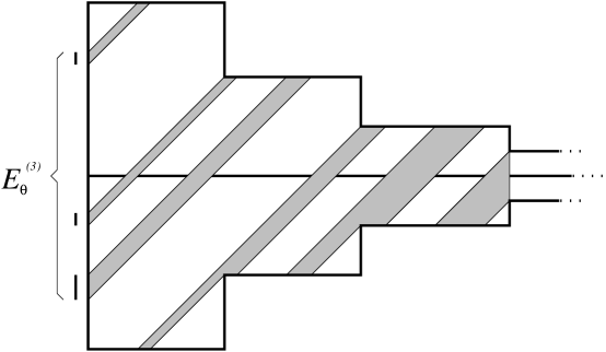
Figure 4: Construction of $E_{\vartheta}^{(n)}$ as the backward evolution of the “aperture” $G_{n}$. The beam of orbits may split at singular vertices.

It is now easy to see that [DDL]:

1. The backward evolution of $G_{n}$ can only split once for each of the $n-1$ singular vertices (Fig. 4). This implies that $E_{\vartheta}^{(n)}$ is the union of at most $n$ right-open intervals. We denote this by $n.i.(E_{\vartheta}^{(n)})\leq n$, where $n.i.$ stands for “number of intervals”.

2. $|E_{\vartheta}^{(n)}|=2p_{n}$.

3. $E_{\vartheta}^{(n+1)}\subset E_{\vartheta}^{(n)}$. In particular, the family $\{E_{\vartheta}^{(n)}\}_{n>0}$ can be rearranged into sequences of nested right-open intervals, whose lengths vanish as $n\to\infty$.

4. If $E_{\vartheta}:=\bigcap_{n>0}E_{\vartheta}^{(n)}$ denotes the subset of $L$ on which ${\cal P}_{\vartheta}$ is not defined, then clearly $|E_{\vartheta}|=0$.

5. Each point of $E_{\vartheta}$ is the limit of an infinite sequence of nested vanishing right-open intervals. Moreover, each infinite sequence yields a point of $E_{\vartheta}$, unless the intervals eventually share their right extremes.

Orbits starting at points of $E_{\vartheta}$ will never collide with any vertical side of $S(\vartheta)$ (or $P$) and thus, as $t\to+\infty$, will go to infinity, maintaining a positive constant $X$-velocity. We call them escape orbits.

It turns out that if the “infinite cusp” of a step polygon narrows down very quickly, several interesting facts can be shown:

Theorem 1

If the heights $\{p_{n}\}$ of an infinite step billiard $P$ verify $p_{n+1}\leq\lambda p_{n}$, with

$$0<\lambda<\lambda_{0}:=\frac{\sqrt{6}-1}{5}\simeq 0.290\ldots,$$

then, for almost all directions $\vartheta\in]0,\pi/2[$, there exists a subsequence $\{n_{j}\}$ such that $n.i.(E_{\vartheta}^{(n_{j})})=1$.

Corollary 1

For almost all directions there is exactly one escape orbit.

Let us name $\eta_{\vartheta}$ the (unique) escape orbit. Also, with a certain lack of originality, let us call typical a direction $\vartheta$ for which the above statements hold.

Theorem 1 and Corollary 1 are the analogues of Corollaries 3 and 4 of [DDL], although their proofs, which are to be found in Section 3, are quite different. In our previous article we exploited thoroughly the arithmetic properties of the exponential billiard $p_{n}=2^{-n}$, whereas here, to achieve a certain generality, we use rather rough measure-theoretic estimates on some sets of directions. This is why we are pretty confident that the same results can indeed be proven for a much wider class of billiards (see the proof of Lemma 2 and in particular estimate (3)).

The next two results are also formulated for a billiard as in the statement of Theorem 1.

Lemma 1

For a.a. $\vartheta$, $\eta_{\vartheta}$ does not intersect any vertex.

The above lemma, too, is proven in Section 3. Not only does it describe the behavior of the escape orbit, but more importantly, in conjunction with Theorem 1, yields the following assertions—which follow from the above in the same way as the entire Section 3 of [DDL] follows from Corollary 3 and Lemma 8.

Proposition 2

Fixed a typical direction $\vartheta$,

• $\eta_{\vartheta}$ is oscillating in the past.

• $\eta_{\vartheta}$ is contained in the $\omega$-limit of every orbit (except for itself).

• $\eta_{\vartheta}$ is contained in the $\alpha$-limit of every orbit (except for the orbit that escapes in the past).

• Excluding the exceptions mentioned above, every semi-orbit stays close to $\eta_{\vartheta}$ for an arbitrary long time.

• Every invariant continuous function on $S(\vartheta)$ is constant.

• The flow is minimal if, and only if, $\eta_{\vartheta}$ is dense.

• The closure of $\eta_{\vartheta}\cap L$, which is the “trace” of the escape orbit on the usual Poincaré section, is either the entire $L$ or a Cantor set.

Remark 4

Proposition 2,(iii) fixes a minor mistake in Corollary 6 of [DDL]: it is obvious that assertion (i) there does not work for the (unique) orbit that escapes in the past.

2.2 Ergodic Properties

We now turn to the ergodic properties of our step billiards, and we start by presenting a slight enhancement of a previous result.

Theorem 2

Fix $\alpha=\tan\vartheta\not\in{\mathbb{Q}}$. For every positive, monotonically vanishing sequence $\{\bar{p}_{n}\}\subset{\mathbb{Q}}$, and every integer $k$, there exists a decreasing sequence $\{p_{n}\}\subset{\mathbb{Q}}$, with

$$p_{n}=\bar{p}_{n}, \mathrm{for}\ 0\leq n\leq k;$$

$$0<p_{n}\leq\bar{p}_{n}, \mathrm{for}\ n>k;$$

$$\sum_{n}p_{n}<\infty.$$

such that the billiard flow $\phi_{\vartheta,t}$ on $S^{P}(\vartheta)$, for $P\simeq\{p_{n}\}$, is ergodic (hence almost all orbits are dense).

Proof. Exactly the same as [DDL], Theorem 1, except that the induction starts at $n=k$. Q.E.D.

Theorem 2 provides an example (many, as a matter of fact) of a billiard that is ergodic in one direction. One would like to get more: a billiard ergodic for a.a. directions, like the rectangular table. We adapt to the infinite step billiards some of the techniques presented in [Tr] to show that this is true “in general”, in the sense of [KMS].

More precisely, let ${\cal S}$ be the space of all step polygons with unit area. (This means that, in this section, we drop the unsubstantial requirement $p_{0}=1$.) Since each step polygon $P$ is uniquely determined by the sequence of the heights of its vertical sides $\{p_{n}\}_{n\in{\mathbb{N}}}$, we apply to ${\cal S}$ the metric of the space $l^{1}$: given $P\simeq\{p_{n}\}$, $Q\simeq\{q_{j}\}$, let

$$d(P,Q):=\sum_{n=0}^{\infty}|p_{n}-q_{n}|.$$

The metric space $({\cal S},d)$ is complete and separable. Note that $d(P,Q)=A(P\triangle Q)$.

We call a set of a topological space typical if it contains a dense $G_{\delta}$-set, meager if it is the union of a countable collection of nowhere dense sets. The following statement is the highlight of this section:

Theorem 3

A typical step polygon $P$ is ergodic on $S^{P}(\vartheta)$ for a.e. $\vartheta\in]0,\pi/2[$.

Corollary 2

There are infinite step billiards $P$ ergodic on $S^{P}(\vartheta)$ for a.e. $\vartheta\in]0,\pi/2[$.

Both results are proven in Section 4. The main differences between Theorem 3 and Theorem 5.1 of [Tr] are:

1. He came first.

2. The result in [Tr] is about a broad class of rational infinite polygons, while ours is restricted to the infinite step polygons.

3. Even though they use the same ideas, Theorem 3 cannot be derived by its analogue in [Tr].

4. His billiards are bounded; ours can be unbounded.

5. The metric that we use is very simple and corresponds to the intuitive idea of closeness.

2.3 Metric Entropy

Let $P\simeq\{p_{n}\}$ be a given infinite step billiard. We denote by ${\cal V}=\{V_{k}\}$ the set of non-removable (singular) vertices, defined at the beginning of Section 2. One can prove the following property of non-periodic orbits, which turns out to be very useful in certain entropy estimates.

Proposition 3

The closure of the forward and backward semi-orbit of every non-periodic point intersects ${\cal V}\cup\{\infty\}$.

Remark 5

This result can be considered the adapted version of Proposition 4.1 in [Tr]. Notice that in our case the billiard is always rational (or weakly rational according to [Tr], Definition 4.3) and ${\cal V}$ is only a subset of all vertices. Also, it is immediate to check that for billiards as in Section 2.2, Proposition 3 is contained in Proposition 2.

Proof of Proposition 3. If a semi-orbit $\gamma$ (either forward or backward) of a non-periodic point is bounded, then it is entirely contained in a finite step billiard $P^{(n)}$, for $n$ large enough. According to [GKT], the closure of $\gamma$ must contain a singular vertex of $P^{(n)}$, which clearly is in ${\cal V}$. If instead $\gamma$ is unbounded, then the set of its limiting points contains $\{\infty\}$. Q.E.D.

Take $n\geq 1$. In Fig. 2, let $L_{n}:=\{n\}\times[p_{n},p_{n-1}[$ and $L_{-n}:=\{n\}\times[-p_{n-1},-p_{n}[$ be the two copies of the $n$-th vertical side. We identify them with $d_{n}:=[p_{n},p_{n-1}[$ and $d_{-n}:=[-p_{n-1},-p_{n}[$. The family of these intervals partitions $I:=[-1,0[\cup]0,1[$. Thus it makes sense to define $f_{\vartheta}$, as the i.e.t. induced by $\phi_{\vartheta,t}$ on $I$.

For any $f_{\vartheta}$-invariant Borel probability measure $\nu$, we set

$$H_{\nu}(P):=-\sum_{n=1}^{\infty}\,\nu(d_{n})\,\log\nu(d_{n}).$$

Call ${\widetilde{\cal X}}_{\vartheta}:=L\setminus\bigcap_{n=0}^{\infty}{\cal P}_{\vartheta}^{-n}E_{\vartheta}$ the set of the points in $L$ whose forward orbits keep returning there; and denote by ${\cal X}_{\vartheta}$ the corresponding set in $I$. More precisely,

$${\cal X}_{\vartheta}:=g_{\vartheta}\left({\widetilde{\cal X}}_{\vartheta}\right),$$

where $g_{\vartheta}\,:\,{\widetilde{\cal X}}_{\vartheta}\longrightarrow I$ is given by $g_{\vartheta}(x)=\phi_{\vartheta,t_{1}}(x)$ and $t_{1}$ is the first collision time at a vertical wall. For any $x\in{\widetilde{\cal X}}_{\vartheta}$, let

$${\widetilde{\pi}}_{\vartheta}(x):=\{\ldots,L_{\omega_{-1}},L,L_{\omega_{0}},L,L_{\omega_{1}},L,\ldots,L,L_{\omega_{k}},\ldots\},$$

be the sequence of vertical sides that the orbit of $x$ crosses (adopting the convention that $L_{\omega_{0}}$ is the first vertical side encountered in the past). Then we define the coding $\pi_{\vartheta}\,:\,{\widetilde{\cal X}}_{\vartheta}\longrightarrow({\mathbb{Z}}^{*})^{{\mathbb{Z}}}$ by

$$\pi_{\vartheta}(x):=\{\ldots,\omega_{-1},\omega_{0},\omega_{1},\ldots\}$$

We equip $C_{\vartheta}:=\pi_{\vartheta}({\cal X}_{\vartheta})$ with the product topology and we denote by $\sigma$ the left shift. The following diagram commutes:

$$\begin{array}[]{ccc}f_{\vartheta}:{\cal X}_{\vartheta}&\longrightarrow&{\cal X}_{\vartheta}\\ \ \quad\uparrow&g_{\vartheta}&\uparrow\\ {\cal P}_{\vartheta}:{\widetilde{\cal X}}_{\vartheta}&\longrightarrow&{\widetilde{\cal X}}_{\vartheta}\\ \ \quad\downarrow&\pi_{\vartheta}&\downarrow\\ \sigma:C_{\vartheta}&\longrightarrow&C_{\vartheta}\end{array}$$

Proposition 4

Let $\nu$ be any $f_{\vartheta}$-invariant, Borel, ergodic probability measure on ${\cal X}_{\vartheta}$. If $H_{\nu}(P)<\infty$, then $h_{\nu}=0$.

Remark 6

For instance, if $p_{n}$ decays exponentially or faster, as in the examples that we have recalled earlier, then $H_{\ell}(P)$ is finite for the Lebesgue measure $\ell$.

Proof of Proposition 4. First of all, notice that the assertion is obvious if $\nu$ is atomic. We claim that the partition $\alpha:=\{\alpha_{1},\alpha_{2},\ldots\}$ given by

$$\alpha_{j}:=\{\omega\in C_{\vartheta}\>\big{|}\>\omega_{1}\,=\,j\}$$

is a one-side generator. This implies by standard results (e.g., [R], 11.3) that $h_{\lambda}=0$ for any $\sigma$-invariant Borel probability measure $\lambda$ on $C_{\vartheta}$. Now, $g_{\vartheta}$ is bijective by construction, therefore the pull-back $g_{\vartheta*}\nu$ is also non-atomic and ergodic. Hence, there is a $Y\subseteq{\widetilde{\cal X}}_{\vartheta}$ such that $\pi_{\vartheta}|_{Y}$ is injective and $g_{\vartheta*}\nu(Y)=1$. We conclude that $h_{\nu}(f_{\vartheta})=h_{\pi_{\vartheta}^{*}g_{\vartheta*}\nu}(\sigma)=0$.

It remains to prove the initial claim. This is done if we show that the sequence of sides an orbit visits in the future determines the sequence of sides visited in the past. Clearly, if the orbit is periodic, there is nothing to prove. In the non-periodic case we can use Proposition 3 to conclude that any parallel strip of orbits must eventually “split” at some vertex $V_{k}$ and this of course implies that two distinct orbits cannot hit the same vertical sides in the future. Q.E.D.

We now turn to the proofs of the other results.

3 Escape orbits

In this section we denote directions by $\alpha=\tan\vartheta\in]0,+\infty[$, using the Lebesgue measure there. All surfaces $S(\alpha)$ will be identified with the set $S$ of Fig. 2 on which we use the coordinates $(X,Y)$. For instance, $\gamma_{k}(\alpha)$ will denote the orbit on $S(\alpha)$ starting at point the $(k,-p_{k})\simeq V_{k}$—this is the same as the orbit on $S$ starting at $(k,-p_{k})$ with slope $\alpha$.

Proof of Theorem 1. Let $k<m$ be two natural numbers. We introduce the following sets:

$$A_{k,m} := \{\alpha\>\big{|}\>\gamma_{k}(\alpha)\mbox{ reaches directly }G_{m}\};$$ (1)

$$B_{m} := \bigcup_{k=1}^{m-1}A_{k,m}.$$ (2)

Therefore,

$$B_{m}^{c}=\{\alpha\>\big{|}\>\mbox{no }\gamma_{k}(\alpha),\mbox{ with }1\leq k\leq m-1,\mbox{ reaches directly }G_{m}\}.$$

Also, let us define

$$C := \bigcap_{n\in{\mathbb{N}}}\bigcup_{m\geq n}B_{m}^{c}=$$

$$= \{\alpha\>\big{|}\>\exists\>\{n_{j}\}\ s.t.\ G_{n_{j}}\mbox{ is not reached by any }\gamma_{k}(\alpha),k\leq n_{j}\}.$$

When such a subsequence exists, the backward evolution of $G_{n_{j}}$ does not split at any of the vertices $V_{k},\,1\leq k\leq n_{j}$. Hence $n.i.(E_{\alpha}^{(n_{j})})=1$. Therefore establishing the theorem amounts to proving that $|C^{c}|=0$. This is implied by the following:

$$\forall\in{\mathbb{N}},\quad\left|\bigcap_{m\geq n}B_{m}\right|=0.$$ (3)

In order to obtain (3), we introduce some notation, and a lemma. Given two sets $A,I$, with $I$ bounded, denote $|A|_{I}:=|A\cap I|/|I|$.

Lemma 2

Assumptions and notations as in Theorem 1. For every (bounded) interval $I\subset{\mathbb{R}}^{+}$, there exists a $\delta\in]0,1[$ such that $\limsup_{m\to\infty}|B_{m}|_{I}\leq\delta$.

The proof of this lemma will be given in the sequel. Now, proceeding by contradiction, let us suppose that $\left|\bigcap_{m\geq n}B_{m}\right|\neq 0$, for some $n$. By the Lebesgue’s Density Theorem, almost all points of that set are points of density. Pick one: this means that there exists an interval $I$, around that point, such that

$$\left|\bigcap_{m\geq n}B_{m}\right|_{I}\geq\sigma>\delta.$$

Hence, $\forall m\geq n,\ |B_{m}|_{I}\geq\sigma$, which contradicts the lemma. This proves (3) and Theorem 1. Q.E.D.

Proof of Corollary 1. The previous theorem implies that, for a.a. $\alpha$’s, $\#E_{\alpha}=$ 0 or 1. As already mentioned, the former case (no escape orbits), occurs if, and only if, the intervals $E_{\alpha}^{(n_{j})}$ share their right extremes, for $j$ large. This implies the existence of generalized diagonals (see Fig. 5). Excluding those cases only amounts to removing a null-measure set of directions. Q.E.D.

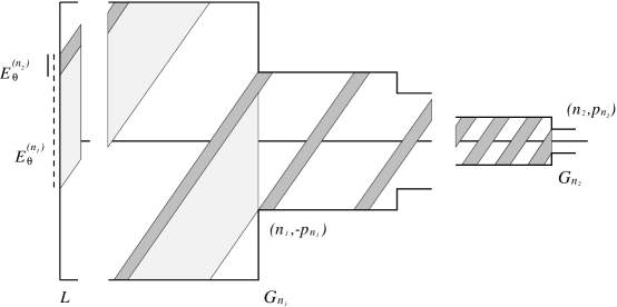
Figure 5: The fact that $E_{\vartheta}^{(n_{1})}$ and $E_{\vartheta}^{(n_{2})}$ have upper (equivalently right) extremes in common implies the existence of a generalized diagonal.

Proof of Lemma 2. In this proof we will heavily use the technique of billiard-unfolding; that is, in order to draw an orbit as a straight line in the plane, we reflect the billiard around one of its sides every time the orbit hits it, as shown in Fig. 6.

Figure 6: Unfolding of the billiard. Trajectories departing from a given singular vertex $V_{k}$ are drawn as straight lines on the plane. Every time one of these hits a side of the billiard, a new copy of the billiard, reflected around that side, is drawn. Cones $I$ and $D_{k+1}$ are used in the proof of Lemma 2.

Fix $k$, and view $I$ as a conical beam of trajectories departing from $V_{k}$ (Fig. 6): this makes sense since these trajectories are in one-to-one correspondence with their slopes. The goal is to exploit the geometry of the unfolded billiard to set up a recursive argument that will yield exponential bounds for $|A_{k,m}|_{I}$ (in $m$).

Here our recursive argument starts. In the unfolded-billiard plane, sketched in Fig. 7, let $l_{k}(\alpha)$ be the straight line of slope $\alpha$ passing through $V_{k}$. Take an $n>k$ and consider one copy of $G_{n}$, indicated as an “opening” in Fig. 7: $\widetilde{G}_{n}:=\{n\}\times[r-p_{n},r+p_{n}[$, for some $r\in{\mathbb{R}}^{+}$. The straight lines (departing from $V_{k}$) that cross $\widetilde{G}_{n}$ encounter a $2p_{n}$-periodic array of copies of $G_{n+1}$. We call them $\widetilde{G}_{n+1}^{(j)}:=\{n+1\}\times[r-p_{n+1}+j\cdot 2p_{n},r+p_{n+1}+j\cdot 2p_{n}[$; $j$ assumes a finite number (say $\ell$) of integer values. Define the interval

$$D_{n}:=\{\alpha\>\big{|}\>l_{k}(\alpha)\cap\widetilde{G}_{n}\neq\emptyset\}.$$ (4)

Figure 7: Proof of Lemma 2: construction of the cones $D_{n}$ and $E_{n}$ in a roughly sketched unfolded-billiard plane.

Remark 7

It might be convenient to think of the elements of $D_{n}$ as lines sharing the common point $V_{k}$: specifically the lines in $D_{n}$ are those that cross $\widetilde{G}_{n}$. So it makes sense to refer to $D_{n}$ (and similar sets) as a cone. (Incidentally, $|D_{n}|=2p_{n}/(n-k)$.) On the other hand, the one-to-one correspondence between $\alpha\in{\mathbb{R}}^{+}$ and $\gamma_{k}(\alpha)$, on one side, and $l_{k}(\alpha)$, on the other, should not lead one to think that the latter is the “lifting” of the former by means of the unfolding procedure. This is only the case when $\gamma_{k}(\alpha)$ reaches $G_{n}$. As a matter of fact, the inclusion $A_{k,n}\cap D_{n}\subseteq D_{n}$ is expected to be strict for general choices of $D_{n}$, $n>k+1$.

The cone $D_{n}$ cuts a segment on the vertical line $y=n+1$. This segment includes some $\widetilde{G}_{n+1}^{(j)}$ and only intersects some other $\widetilde{G}_{n+1}^{(i)}$ (at most two, of course). Now expand $D_{n}$ in such a way that the segment includes $\ell$ “full” copies of $G_{n+1}^{(j)}$; the resulting cone will be denoted by $E_{n}$. Fig. 7 shows that in this operation we might have to attach, on top and on bottom of $D_{n}$ two cones of measure up to $2p_{n+1}/(n+1-k)$. Therefore:

$$\frac{|E_{n}|}{|D_{n}|}\leq 1+\frac{4p_{n+1}}{(n+1-k)|D_{n}|}\leq\frac{2p_{n+1}+p_{n}}{p_{n}}.$$ (5)

We further define the set

$$D_{n+1}:=\{\alpha\in E_{n}\>\big{|}\>l_{k}(\alpha)\cap\widetilde{G}_{n+1}^{(j)}\neq\emptyset,\mbox{ for some }j\}=\bigcup_{i=1}^{\ell}D_{n+1}^{(i)},$$ (6)

where the $D_{n+1}^{(i)}$ are cones of measure $2p_{n+1}/(n+1-k)$. One has:

$$\frac{|D_{n+1}|}{|E_{n}|}\leq\frac{2\cdot 2p_{n+1}}{2\cdot 2p_{n+1}+2(p_{n}-p_{n+1})}=\frac{2p_{n+1}}{p_{n+1}+p_{n}}.$$ (7)

In fact it is not hard to realize that the l.h.s. of (7) is largest when $\ell=2$. In that case, $E_{n}\setminus D_{n+1}$ is a interval of measure $2(p_{n}-p_{n+1})/(n+1-k)$, whence the second term of (7). Combining (5) and (7) we obtain

$$\frac{|D_{n+1}|}{|D_{n}|}\leq\frac{2p_{n+1}(2p_{n+1}+p_{n})}{p_{n}(p_{n+1}+p_{n})}=:\beta_{n}.$$ (8)

At this point we notice that each $D_{n+1}^{(i)}$ as introduced in (6) is again a set of the type (4), with $n+1$ replacing $n$. Hence estimate (8) holds and $|D_{n+2}^{(i)}|\leq\beta_{n+1}|D_{n+1}^{(i)}|$ with $D_{n+2}^{(i)}$ suitably defined as in the above construction. Call $D_{n+2}=\cup_{i=1}^{\ell}D_{n+2}^{(i)}$: this set is also a union of cones of equal size. One has

$$\frac{|D_{n+2}|}{|D_{n+1}|}\leq\frac{\sum_{i=1}^{\ell}|D_{n+2}^{(i)}|}{\ell\,|D_{n+1}^{(i)}|}\leq\beta_{n+1},$$

and the trick can continue.

We are now ready to implement the recursive argument: assume that some of the orbits of the cone $I$ (based in $V_{k}$) cross $G_{k+1}$, that is, $A_{k,k+1}\cap I\neq\emptyset$ (if not, everything becomes trivial as we will see later). In the unfolded-billiard plane, enlarge $A_{k,k+1}\cap I$ until it fits the minimal number of copies of $G_{k+1}$, as in Fig. 6; call this new set $D_{k+1}$. This is by definition a finite union of intervals of the type (4), of fixed size). Hence inequality (8) applies and the definition/estimate algorithm can be carried on until we define, say, $D_{m}$. The only thing we need to know about this set is that $(A_{k,m}\cap I)\subseteq D_{m}$, which should be clear by construction (see also the previous remark). This fact and the repeated use of (8), yield

$$|A_{k,m}\cap I|\leq|D_{k+1}|\prod_{i=k+1}^{m-1}\beta_{i}.$$ (9)

Let us consider our specific case: $p_{n+1}\leq\lambda p_{n}$. From definition (8), one verifies that:

$$\beta_{n}=\frac{2(2(p_{n+1}/p_{n})+1)}{((p_{n}/p_{n+1})+1)}\leq\frac{2(2\lambda+1)}{\lambda^{-1}+1}=:\beta.$$ (10)

It is going to be crucial later that $\beta$ be less than 1. For $\lambda$ positive, this amounts to $4\lambda^{2}+\lambda-1<0$, which is easily solved by

$$0<\lambda<\lambda_{1}:=\frac{\sqrt{17}-1}{8}\simeq 0.390\ldots,$$ (11)

Going back to the definition of $D_{k+1}$, and to (9), we see that it is possible to give an estimate of the measure of $D_{k+1}$ in $I$, for large $k$. In fact, when $|I|$ is much bigger than $2p_{k}$, then it is clear (from Fig. 6, say) that $I$ includes very many cones of size $2p_{k+1}$, placed on a $2p_{k}$-periodic array. As $k$ grows, the density of these cones in $I$ can be made arbitrarily close to $p_{k+1}/p_{k}\leq\lambda$. The precise statement then is: given any $\varepsilon>0$, there exists a $q=q(\varepsilon)\in{\mathbb{N}}$ such that

$$\forall k\geq q,\quad|D_{k+1}|<(\lambda+\varepsilon)\,|I|.$$

Plugging this into (9), we obtain

$$\forall m>k\geq q\quad|A_{k,m}|_{I}\leq(\lambda+\varepsilon)\,\beta^{m-k-1},$$ (12)

having used (10) as well. For the other values of $k$, we have no control over $C_{k}:=|D_{k+1}|/|I|$ and we just write

$$\forall m,q>k\quad|A_{k,m}|_{I}\leq C_{k}\,\beta^{m-k-1}.$$ (13)

In the case $A_{k,k+1}\cap I=\emptyset$, which we did not consider before, (12)-(13) are trivial consequences of the fact that $A_{k,m}\cap I=\emptyset$, for all $m>k$.

We move on to the final estimation. Take $m>q$: from definition (2) we have, using (12) and (13),

$$|B_{m}|_{I} \leq \sum_{k=1}^{q-1}|A_{k,m}|_{I}+\sum_{k=q}^{m-1}|A_{k,m}|_{I}\leq$$

$$\leq \sum_{k=1}^{q-1}C_{k}\,\beta^{m-k-1}+\sum_{k=q}^{m-1}(\lambda+\varepsilon)\,\beta^{m-k-1}\leq$$

$$\leq o(1)+\frac{\lambda+\varepsilon}{1-\beta},$$

as $m\to\infty$. In the last inequality we have used twice the fact that $\beta<1$. We impose the condition

$$\frac{\lambda}{1-\beta}=\frac{\lambda(\lambda+1)}{-4\lambda^{2}-\lambda+1}<1.$$ (15)

For $\lambda$ as in (11), the denominator is positive, hence (15) can be rewritten as $5\lambda^{2}+2\lambda-1<0$, whose solutions are

$$0<\lambda<\frac{\sqrt{6}-1}{5}=\lambda_{0}<\lambda_{1},$$ (16)

as in the statement of the lemma. For these values of $\lambda$, by virtue of (11), $1-\beta$ keeps away from 0. Therefore (15) implies that, for $\varepsilon$ small enough, the last term in (3) can be taken less than a certain $\delta<1$, whence the proof of Lemma 2. Q.E.D.

Proof of Lemma 1. Consider a vertex $V$ of $P_{\alpha}$ and let $\gamma_{V}(\alpha)$ be its forward semi-orbit. For a fixed finite sequence $S:=(S_{1},S_{2},\ldots S_{\ell})$ of sides, we define

$$A_{V,m}(S):=\{\alpha\>\big{|}\>\gamma_{V}(\alpha)\mbox{ hits }S_{1},\ldots,S_{\ell}\mbox{ and then reaches directly }G_{m}\}.$$ (17)

This means that these trajectories do not hit any vertical wall after leaving $S_{\ell}$ and before reaching $G_{m}$. Notice the similarities with definition (1). As a matter of fact, if $V=V_{k}$ for some $k$, then $A_{V_{k},m}(\emptyset)=A_{k,m}$. However, for most sequences $S$, (17) defines the empty set. For example, $S$ can be incompatible in the sense that no orbit can go from $S_{i}$ to $S_{i+1}$ without crossing other sides in the meantime. But, even for compatible sequences, if $G_{m}$ does not lie to the right of $S_{\ell}$, obviously $A_{V,m}(S)=\emptyset$. To avoid this latter case, we fix $m_{o}=m_{o}(V,S)$ bigger than the largest $Y$-coordinate in $S_{\ell}$. For $m\geq m_{o}$, $A_{V,m+1}(S)\subset A_{V,m}(S)$. Let us then define

$$B_{V}(S) := \{\alpha\>\big{|}\>\gamma_{V}(\alpha)\mbox{ hits }S_{1},\ldots,S_{\ell}\mbox{ and then escapes to }\infty\}=$$ (18)

$$:= \bigcap_{m=m_{o}}^{\infty}A_{V,m}(S),$$

Working in the unfolded-billiard plane and identifying directions with orbits, it is not hard to realize that $A_{V,m_{o}}(S)$ is made up of a finite number of intervals/cones, each of which reaches a copy of $G_{m_{o}}$ after hitting a certain sequence of sides $(S_{1},\ldots S_{\ell},S_{\ell+1},\ldots S_{n})$ (the first $\ell$ sides are common to all cones and the others can only be horizontal). It is possible that some of these beams of trajectories intersect the corresponding copy of $G_{m_{o}}$ only in a proper sub-segment. Let us fix this situation by enlarging any such beam until it covers the whole segment. We call $D\supseteq A_{V,m_{o}}(S)$ the union of these new cones.

Proceeding exactly as in the proof of Lemma 2 (see in particular (9) and (13)) we get, for $m>m_{o}$,

$$|A_{V,m}(S)|\leq|D|\,\beta^{m-m_{o}},$$

with $\beta<1$. Hence, for $m\to\infty$, $|A_{V,m}(S)|\to 0$. By (18), $|B_{V}(S)|=0$, and the set

$$\bigcup_{V\atop\mathrm{vertex}}\bigcup_{S\ \mathrm{finite}\atop\mathrm{sequence}}B_{V}(S)$$

has measure zero. This is the set of directions as in the statement of the Lemma 2, which we have now proved. Q.E.D.

4 Generic ergodicity

We begin this section by giving some definitions and a technical lemma. In ${\mathbb{R}}^{2}$, let $\rho$ be the Euclidean metric and $A$ the area. Also, recall the definition of ${\cal S}$ from Section 2.2; later on we will need to use ${\cal S}_{0}$, the collection of all finite $P\in{\cal S}$ with rational heights.

Definition 1

Given $P,Q\in{\cal S}$, $\vartheta\in]0,\pi/2[$, $x\in S^{P}(\vartheta)\cap S^{Q}(\vartheta)$ and $\varepsilon>0$, let

$$I(P,Q,x,\varepsilon):=\{t\in[0,1/\varepsilon]\>\big{|}\>\rho(\phi_{t}^{P}(x),\phi_{t}^{Q}(x))>\varepsilon\},$$ (19)

$$G(P,Q,\vartheta,\varepsilon):=\{x\in S^{P}(\vartheta)\cap S^{Q}(\vartheta)\>\big{|}\>|I(P,Q,x,\varepsilon)|<\varepsilon\},$$ (20)

$$E(P,Q,\varepsilon):=\left\{\vartheta\in]0,\pi/2[\>\big{|}\>A(G(P,Q,\vartheta,\varepsilon))\geq A(S^{P,Q}(\vartheta))-\varepsilon\right\}.$$ (21)

Lemma 3

For any $P\in{\cal S}$ and $\varepsilon>0$, we have

$$\lim_{Q\rightarrow P}|E(P,Q,\varepsilon)|=1.$$

Proof of Lemma 3. It is enough to prove the statement for any sequence converging to $P$. Let $\{P_{n}\}$ be such a sequence. Fix $\vartheta\in]0,\pi/2[$ and $\varepsilon>0$. Only countably many orbits of $S^{P}(\vartheta)$ contain a singular vertex $V$. Let $x\in S^{P}$ be a point that does not belong to any of these orbits. In a finite interval of time, its trajectory can get close only to a finite number of singular vertices. Therefore $\delta_{\varepsilon}$, the distance between the $\cup_{0\leq t\leq 1/\varepsilon}\,\phi_{\vartheta,t}^{P}(x)$ and $\mathcal{V}$, is positive. Let $N_{\varepsilon}$ be the number of collisions of $\cup_{0\leq t\leq 1/\varepsilon}\,\phi_{\vartheta,t}^{P}(x)$ with the horizontal sides of $S^{P}(\vartheta)$.

The two surfaces $S^{P}(\vartheta)$ and $S^{P_{n}}(\vartheta)$ overlap (as subsets of ${\mathbb{R}}^{2}$). If $x\in S^{P_{n}}$ as well, then the set $\cup_{0\leq t\leq 1/\varepsilon}\,\phi_{\vartheta,t}^{P_{n}}(x)$ represents a finite piece of the trajectory of $x$ in the surface $S^{P_{n}}(\vartheta)$. We want to estimate $\rho(\phi^{P}_{t}(x),\phi^{P_{n}}_{t}(x))$ for $0\leq t\leq 1/\varepsilon$. Since there is a natural correspondence between the sides of the two surfaces, when we say that the two trajectories hit the same sequence of sides, we mean corresponding sides. Notice that $\rho(\phi^{P}_{t}(x),\phi^{P_{n}}_{t}(x))$ stays constant when neither orbit crosses any sides. Also, as long as $\phi^{P}_{t}(x)$ and $\phi^{P_{n}}_{t}(x)$ hit the same sequence of sides, every time that there is collision at a horizontal side, the distance $\rho(\phi^{P}_{t}(x),\phi^{P_{n}}_{t}(x))$ increases by a term $h\leq 2d(P,P_{n})$. Hence the maximum distance between the two trajectories in the interval $t\in[0,1/\varepsilon]$ is $\leq 2d(P,P_{n})N_{\varepsilon}$. Therefore, by definition of $\delta_{\varepsilon}$, if $d(P,P_{n})<\delta_{\varepsilon}/(2N_{\varepsilon})$, the trajectories encounter the same sequence of sides for $0\leq t\leq 1/\varepsilon$.

Since $d(P,P_{n})\rightarrow 0$ as $n\rightarrow\infty$, we can find an $m(x,\varepsilon)>0$ such that the previous inequality is satisfied for all $n>m(x,\varepsilon)$. It is clear now that, as $n$ grows larger, the distance between the two trajectories decreases. We conclude that, for points $x\in S^{P}(\vartheta)$ with non-singular positive semi-trajectory,

$$\lim_{n\to\infty}\,\max_{0\leq t\leq 1/\varepsilon}\rho(\phi^{P}_{t}(x),\phi^{P_{n}}_{t}(x))=0.$$

As a consequence we have that a.e. $x\in S^{P}(\vartheta)$ belongs to $G(P,P_{n},\vartheta,\varepsilon)$ if $n$, which depends on $x$, is sufficiently large. Therefore $A(G(P,P_{n},\vartheta,\varepsilon))\to A(S^{P}(\vartheta))$ as $n\to\infty$. Being this true for all $\vartheta\in]0,\pi/2[$, we finally obtain $|E(P,P_{n},\varepsilon)|\to 1$ as $n\to\infty$, for any $\varepsilon>0$. Q.E.D.

We are now in position to attack the main proof of this section:

Proof of Theorem 3. Choose $\varepsilon_{n}>0$ such that $\lim_{n\to\infty}\varepsilon_{n}=0$. Let $\{f_{i}\}_{i\in{\mathbb{N}}}$ be a countable collection of continuous functions with compact support and let it be dense in $L^{1}({\mathbb{R}}^{2})$. For each step polygon $P$, $f_{i}^{P}$ denotes the restriction of $f_{i}$ to $S^{P}(\vartheta)$, corrected to obey the identifications on $S^{P}(\vartheta)$. These corrections occur on a set of zero Lebesgue measure in ${\mathbb{R}}^{2}$, therefore $\{f^{P}_{i}\}_{i\in{\mathbb{N}}}$ is dense in $L^{1}(S^{P}(\vartheta))$ for each $\vartheta\in]0,\pi/2[$.

Given $P\in{\cal S}$, $x\in S^{P}(\vartheta)$ and $i\in{\mathbb{N}}$, let us introduce

$$B_{T}^{P}(\vartheta,i,x):=\left|\frac{1}{T}\int_{0}^{T}f_{i}^{P}\circ\phi^{P}_{t}(x)dt-\frac{1}{A(S^{P}(\vartheta))}\int_{S^{P}(\vartheta)}f_{i}^{P}dA\right|$$

and

$$C_{T}^{P}(\vartheta,n):=\left\{x\in S^{P}(\vartheta)\>\big{|}\>B_{T}^{P}(\vartheta,i,x)\leq\varepsilon_{n},\>i=1,\ldots,n\right\}.$$

If $P\in{\cal S}_{0}$, the billiard flow $\phi_{\vartheta,t}^{P}$ is uniquely ergodic for all irrational $\vartheta$ (i.e., $\tan\vartheta\not\in{\mathbb{Q}}$). Thus for every $n>0$ and every irrational $\vartheta\in]0,\pi/2[$, we have that $\lim_{T\to+\infty}A(C_{T}^{P}(\vartheta,n))=A(S^{P}(\vartheta))$. Let

$$D_{T}^{P}(n):=\left\{\vartheta\in]0,\pi/2[\>\big{|}\>A(C^{P}_{T}(\vartheta,n))\geq A(S^{P}(\vartheta))-\varepsilon_{n}\right\}.$$

Then we can choose a $T_{n}(P)\geq n$ such that $|D_{T}^{P}(n)|>1-\varepsilon_{n}$ for any $T\geq T_{n}(P)$. Since $f_{1},f_{2},\ldots,f_{n}$ are uniformly continuous on ${\mathbb{R}}^{2}$, there is an $r_{n}>0$ for which $|f_{i}(x)-f_{i}(y)|\leq\varepsilon_{n}$ whenever $\rho(x,y)\leq r_{n}$ and $i=1,\ldots,n$. Let

$$\delta_{n}(P):=\min\left\{\frac{1}{T_{n}(P)},\varepsilon_{n},\frac{\varepsilon_{n}}{\max_{1\leq i\leq n}\|f_{i}\|_{\infty}},r_{n}\right\}$$

and $\tau_{n}:=1/\delta_{n}$. According to Lemma 3, there exists $0<\sigma_{n}(P)\leq\delta_{n}(P)$ such that if $Q\in U_{\sigma_{n}}(P):=\{R\in{\cal S}\>\big{|}\>d(P,R)\leq\sigma_{n}\}$, then $|E(P,Q,\delta_{n})|>1-\delta_{n}\geq 1-\varepsilon_{n}$.

Let $E_{n}:=E(P,Q,\delta_{n})$ and $I_{n}(x)$, $G_{n}(\vartheta)$ be the sets (19), (20) used in the definition of $E(P,Q,\delta_{n})$. These sets depend on $P$. For $\vartheta\in E_{n}$ and $x\in G_{n}(\vartheta)$, $A(G_{n}(\vartheta))\geq A(S^{P,Q}(\vartheta))-\delta_{n}\geq A(S^{P,Q}(\vartheta))-\varepsilon_{n}$, $|I_{n}(x)|<\delta_{n}$ and $\rho(\phi^{P}_{t}(x),\phi^{Q}_{t}(x))\leq\delta_{n}\leq r_{n}$ for $t\in[0,\tau_{n}]\setminus I_{n}(x)$. Notice that $T_{n}\leq\tau_{n}$. For $i=1,\ldots,n$, we have:

$$\left|\frac{1}{A(S^{P})}\int_{S^{P}}f_{i}^{P}dA-\frac{1}{A(S^{Q})}\int_{S^{Q}}f_{i}^{Q}dA\right|=$$

$$\qquad=\frac{1}{A(S^{P})}\left|\int_{S^{P}}f_{i}^{P}dA-\int_{S^{Q}}f_{i}^{Q}dA\right|\leq$$ (22)

$$\qquad\leq\frac{1}{4}\int_{S^{P}\triangle S^{Q}}\left|f_{i}\right|dA\leq\frac{1}{4}\|f_{i}\|_{\infty}A(S^{P}\triangle S^{Q})\leq$$

$$\qquad\leq\sigma_{n}\|{f_{i}}\|_{\infty}\leq\delta_{n}\|{f_{i}}\|_{\infty}\leq\varepsilon_{n}.$$

Let $\vartheta\in D_{\tau_{n}}^{P}(n)\cap E_{n}$ and $x\in C^{P}_{\tau_{n}}(\vartheta,n)\cap G_{n}(\vartheta)$. Then

$$\left|\frac{1}{\tau_{n}}\int^{\tau_{n}}_{0}f_{i}^{Q}\circ\phi_{t}^{Q}(x)dt-\frac{1}{A(S^{Q})}\int_{S^{Q}}f_{i}^{Q}dA\right|$$

$$\qquad\leq\frac{1}{\tau_{n}}\int^{\tau_{n}}_{0}\left|f_{i}^{Q}\circ\phi^{Q}_{t}(x)-f_{i}^{P}\circ\phi^{P}_{t}(x)\right|dt+$$

$$\qquad+\left|\frac{1}{\tau_{n}}\int^{\tau_{n}}_{0}f_{i}^{P}\circ\phi^{P}_{t}(x)dt-\frac{1}{A(S^{P})}\int_{S^{P}}f_{i}^{P}dA\right|+$$

$$\qquad+\left|\frac{1}{A(S^{P})}\int_{S^{P}}f_{i}^{P}dA-\frac{1}{A(S^{Q})}\int_{S^{Q}}f_{i}^{Q}dA\right|$$

$$\qquad=:I+II+III.$$

We have $I\leq 2\,\delta^{2}_{n}\|f_{i}\|_{\infty}+\varepsilon_{n}\leq 3\varepsilon_{n}$—say—for $n$ large enough. Moreover, $x\in C^{P}_{\tau_{n}}(\vartheta,n)$ implies $II\leq\varepsilon_{n}$. Finally, $III\leq\varepsilon_{n}$ by (22). We conclude that $I+II+III\leq 5\varepsilon_{n}$ for $\vartheta\in D_{\tau_{n}}^{P}(n)\cap E_{n}$, $x\in C^{P}_{\tau_{n}}(\vartheta,n)\cap G_{n}(\vartheta)$ and $i=1,\ldots,n$. By definition of $D_{\tau_{n}}^{P}(n)$ and $E_{n}$, we have:

$$|D_{\tau_{n}}^{P}(n)\cap E_{n}|>1-2\varepsilon_{n}.$$ (23)

From $A(C^{P}_{\tau_{n}}(\vartheta,n))\geq A(S^{P}(\vartheta))-\varepsilon_{n}$ and $A(G_{n}(\vartheta))\geq A(S^{P}(\vartheta))-\varepsilon_{n}$, it follows that

$$A(C_{\tau_{n}}^{P}(\vartheta,n)\cap G_{n}(\vartheta))\geq A(S^{P}(\vartheta))-2\varepsilon_{n}=A(S^{Q}(\vartheta))-2\varepsilon_{n}.$$ (24)

Let $\{P_{j}\}_{j\in{\mathbb{N}}}$ be an enumeration of ${\cal S}_{0}$ and

$$H:=\bigcap^{\infty}_{n=1}\bigcup^{\infty}_{j=n}U_{\sigma_{n}(P_{j})}(P_{j}).$$

It is easy to see that $H$ is a dense $G_{\delta}$-subset of ${\cal S}$. If $Q\in H$, then for every $n>0$ there is a $j_{n}$ for which $Q\in U_{\sigma_{n}(P_{j_{n}})}(P_{j_{n}})$. Define $D:=\bigcap^{\infty}_{m=1}\bigcup_{n\geq m}D_{\tau_{n}}^{P_{j_{n}}}(n)\cap E_{n}$. By (23), $|D|=1$. This means that, for each $\vartheta\in D$, there is a subsequence $\{n_{k}\}$ such that $\vartheta\in D_{\tau_{n_{k}}}^{P_{j_{n_{k}}}}(n_{k})$ for all $k$. In order to avoid heavy notation, let us denote such a sequence by $\{n\}$. Now call $C(\vartheta):=\bigcap^{\infty}_{m=1}\bigcup_{n\geq m}C_{\tau_{n}}^{P_{j_{n}}}(\vartheta,n)\cap G_{n}(\vartheta)$. From (24), $A(C(\vartheta))=A(S^{Q}(\vartheta))$.

So, for each $\vartheta\in D$ and $x\in C(\vartheta)$ (i.e., a.e. $\vartheta$ and a.e. $x\in S^{Q}(\vartheta)$) there exists a subsequence $\{n_{k}\}$ such that $\lim_{k\to\infty}\tau_{n_{k}}=+\infty$ and

$$\lim_{k\to\infty}\frac{1}{\tau_{n_{k}}}\int_{0}^{\tau_{n_{k}}}f_{i}^{Q}\circ\phi^{Q}_{t}(x)dt=\frac{1}{A(S^{Q})}\int_{S^{Q}}f_{i}^{Q}dA,$$

for all $i\in{\mathbb{N}}$. Since $\{f_{i}^{Q}\}_{i\in N}$ is dense in $L^{1}(S^{Q}(\vartheta))$, using a standard approximation argument, and Birkhoff’s Theorem, we conclude that $\phi_{\vartheta,t}^{Q}$ is ergodic for a.e. $\vartheta\in]0,\pi/2[$. Q.E.D.

Proof of Corollary 2. Let $F^{N}\subset{\mathcal{S}}$ be the collection of finite step polygons with $N$ sides. Each $F^{N}$ is a nowhere dense set in ${\mathcal{S}}$, so the subset of all finite step polygons $F:=\bigcup_{N\geq 4}F^{N}$ is a meager set of ${\mathcal{S}}$. By Baire’s Theorem, $H$ is a set of second category, therefore it intersects the complement of $F$. In other words, $H$ contains infinite step polygons. Q.E.D.

References

- [Ar] P. Arnoux, Ergodicité generique des billards polygonaux, Seminaire Bourbaki 696 (1988), 203-221.
- [B] M. Boshernitzan, Billiards and rational periodic directions in polygons, Amer. Math. Monthly 99(6) (1992), 522-529.
- [DDL] M. Degli Esposti, G. Del Magno and M. Lenci, An infinite step billiard, Nonlinearity 11(4) (1998), 991-1013.
- [FK] R. H. Fox and R. B. Kershner, Concerning the transitive properties of geodesic on a rational polyhedron, Duke Math. J. 2 (1936), 147-150.
- [EFV] B. Eckhardt, J. Ford and F. Vivaldi, Analytically solvable dynamical systems which are not integrable., Phys. D 13(3) (1984), 339-356.
- [G1] E. Gutkin, Billiard flows on almost integrable polyhedral surfaces, Ergod. Th. & Dyn. Sys. 4 (1984), 569-584.
- [G2] E. Gutkin, Billiards in polygons, Physica D 19 (1986) 311-333.
- [G3] E. Gutkin, Billiards in polygons: survey of recent results, J. Stat. Phys. 83 (1996), 7-26.
- [GKT] G. Galperin, T. Krüger and S. Troubetzkoy, Local instability of orbits in polygonal and polyhedral billiards, Comm. Math. Phys. 169 (1995), 463-473.
- [GU] M.-J. Giannoni and D. Ullmo, Coding chaotic billiards. I. Noncompact billiards on a negative curvature manifold, Phys. D 41(3) (1990), 371-390.
- [KMS] S.Kerckhoff, H.Masur and J.Smillie, Ergodicity of billiard flows and quadratic differentials, Ann. Math. 124 (1986), 293-311.
- [KZ] A. Katok and A. Zemlyakov, Topological transitivity of billiards in polygons, Math Notes 18 (1975), 760-764.
- [Le] M. Lenci, Escape orbits for non-compact flat billiards, Chaos 6(3) (1996), 428-431.
- [L] A. M. Leontovich, The existence of unbounded oscillating trajectories in a problem of billiards, Sov. Acad. Sci., doklady Math. 3(4) (1962), 1049-1052.
- [M] H. Masur, Closed trajectories of a quadratic differential, Duke J. Math. 53 (1986), 307-314.
- [PP] Ya. Pesin and B. Pitskel, Topological pressure and the variational principle for noncomapct sets, Func. Anal. Appl. 18 (1984), 307-318.
- [R] V. A. Rokhlin, Lectures on the entropy theory of measure-preserving transformations, Russ. Math. Surv. 22(5) (1967), 1-52.
- [S] Ya. G. Sinai (ed.), Dynamical systems II (Ergodic theory with applications to dynamical systems and statistical mechanics), Encyclopaedia of Mathematical Sciences, 2. Springer-Verlag, Berlin, 1989.
- [T] S. Tabachnikov, Billiards, Société mathématique de France, Paris, 1995.
- [Tr] S. Troubetzkoy, Billiards in infinite polygons, Nonlinearity 12 (1999), 293-311.
- [Tr2] S. Troubetzkoy, Topological transitivity of infinite step billiards, preprint (1999).