Geometrical approach to the distribution of the zeroes for the Husimi function.

Abstract

We construct a semiclassical expression for the Husimi function of autonomous systems in one degree of freedom, by smoothing with a Gaussian function an expression that captures the essential features of the Wigner function in the semiclassical limit. Our approximation reveals the “center and chord” structure that the Husimi function inherits from the Wigner function, down to very shallow valleys, where lie the Husimi zeroes. This explanation for the distribution of zeroes along curves relies on the geometry of the classical torus, rather than the complex analytic properties of the WKB method in the Bargmann representation. We evaluate the zeroes for several examples.

I Introduction

The features that distinguish integrable from chaotic motion in classical mechanics manifest themselves most clearly in phase space. This is one of the reasons for the great interest in the so called “quasiprobability distribution functions” in phase space within the semiclassical theory of quantum states. These distributions are defined as the symbols associated with the density operator $\hat{\rho}$ in some representation of quantum operators [6, 7]. It is expected that these representations of quantum states show the differences between an integrable, or a chaotic classical counterpart in the semiclassical limit ($\hbar\rightarrow 0$). Among these phase space representations of quantum states, the Wigner function (i.e. the symbol of the density operator $\hat{\rho}$ in the Weyl representation) and its smoothing by a Gaussian function, the Husimi function, are of paramount importance. In fact, Berry [1] showed that the peak of the amplitude of the Wigner function is located very close to the curve of constant energy, for a pure state of an autonomous system with one degree of freedom, collapsing onto a zero-width distribution (i.e., a delta function) over that curve in the classical limit ($\hbar=0$) (see also [4, 5, 6]). Ozorio de Almeida and Hannay generalized this picture for states supported by invariant tori of higher dimensions [2]. In all such systems, the semiclassical analysis of the Wigner function [1, 2, 3, 4, 5] reveals an interesting geometrical structure of “chords and centers” that determines the phase of the oscillations of the Wigner function as the point ${\bf x}=(q,p)$ is varied within the torus. This phase is proportional to the symplectic area -or center action- bounded by the torus and the chord, centered on ${\bf x}$, joining two points of the torus. The links of this “semiclassical geometry” to the generating function formalism of classical mechanics and the path integrals of quantum mechanics are reviewed in reference [8].

Although the oscillations of the Wigner function thus reflect legitimate structures of classical mechanics, its positive definite Gaussian smoothing, the Husimi function, is much closer to a classical Liouville density. The density peaks near the region of classical motion, decaying exponentially in classically forbidden regions [14, 15]. The first impression is that smoothing cancels all trace of the centre and chord skeleton of the Wigner function. However, we shall show that very delicate effects are still discernible.

First, we must recall that the Husimi function can also be viewed as the mean value of the density operator $\hat{\rho}$ in coherent states, whose holomorphic (entire) part is called the Bargmann function [9]. This function corresponds to the wave function for the quantum state in a representation of the quantum mechanics introduced by Bargmann [10] (in the case of the Heisenberg-Weyl group), where the basis for the Hilbert space is made of coherent states not normalized to unity. Thus, in the Bargmann representation the wave functions are holomorphic (entire) functions of the variable $z=\frac{1}{\sqrt{2}}(\beta q-ip/\beta)$, acting as a phase space coordinate. The analiticity of the Bargmann function compels its zeroes and those of the Husimi function to be isolated for 1-D systems. Leboeuf and Voros [16] have shown that in many cases the distribution of Husimi zeroes is completely different for chaotic maps, where they are spread out, as opposed to integrable maps, where they are distributed along curves. Only the latter alternative is available for systems with continous time and one degree of freedom. Furthermore, these lines of zeroes cannot occur close to the energy shell where the smoothed Wigner function has a non-oscillatory peak. The lines supporting zeroes may only be found in regions where the Husimi function is already exponentially small.

In these circunstances, we can only expect to predict the general pattern of zeroes with a very delicate “subdominant” semiclassical theory. This is the case of WKB type of theory developed by Voros for the Bargmann representation [9], which predicts zeroes on the anti-stokes lines where two or more branches of the complex action have the same amplitude. The zeroes along these lines are selected by the condition that the imaginary part of the complex action be an integer multiple of $\pi$. However, this approach has practical difficulties to obtain explicit formulae even to leading order in $\hbar$. First, it is generally very difficult to obtain analitically the branches of the classical energy curve in complex coordinates, in order to calculate explicitily the complex action (i.e. the phase in the WKB wave function). Second, an approximation valid anywhere outside the neighborhood of the energy curve, requires the analytic continuation of the functions that define the branches; this needs the analyticity of the Weyl symbol, $H_{W}$, for the quantum Hamiltonian.

Let us thus return to the picture of the Husimi function as a smoothing of the Wigner function. Since our approximation does not maintain explicitily the analytical properties, one could not expect to establish that there exist isolated zeroes in this way, but we can seek for shallow valleys, even in the region where the Husimi function is already exponentially small, and for oscillations along their bottom as indications of where the zeroes may lie. The simplest guess is that the two dominant regions in the evaluation of the Husimi function are the neighborhood of the centre of the Gaussian and the maximum of the Wigner function along the energy curve $\cal E$. Since we know that a zero will only be found when the Gaussian is far removed from the energy curve, we use Berry’s simple cosine-oscillatory representation of the Wigner function for the local approximation. For the contribution of the region near the energy curve, we start from the even cruder classical aproximation that the Wigner function is a $\delta$-function along $\cal E$. After the smoothing, the first term remains cosine-oscillatory with essentially the same phase (proportional to the center action, upon small corrections), but now damped by an exponential function which decreases, essentially with the length of the chords (upon small corrections). The second term is everywhere positive, smooth and peaked in the energy curve $\cal E$. The combination of both produces a positive smooth expression, peaked along the curve $\cal E$ oscillating in a valley of local minima that approach the zeroes of the Husimi function when $\hbar\rightarrow 0$. This expression is valid only inside the energy curve and depends only on the properties of the torus $\cal E$.

The paper is organized as follows. In Section II we summarize important results concerning Wigner and Husimi functions. In Section III we find a semiclassical expression of the Husimi function for the case of a particle in a box, as a simple model of the geometrical approach. In Section IV we introduce our geometrical approach to the distribution of the Husimi zeroes in 1-D systems. In Section V we apply this approach to the problem of a particle under the action of a constant force. This example corresponds to an unbounded problem whose convex energy curve is open. Finally, in Section VI we present the results for the case of a particle subject to an asymmetric anharmonic potencial, as example of a general system with a convex and closed energy curve.

II Review of Wigner and Husimi functions

Quasiprobability distribution functions are symbols associated with the density operator, $\hat{\rho}$, in some representation of quantum operators [6, 7]. The Wigner function is the Weyl symbol of the density operator. The symbol of an operator $\hat{\mbox{A}}$, in the Weyl representation is given by the function,

$$A_{W}({\bf x})=\int d\xi_{q}\;\;\langle q+\xi_{q}/2|\hat{\mbox{A}}|q-\xi_{q}/2\rangle\;\;\exp\left[-ip\xi_{p}/\hbar\right]\;,$$ (1)

where ${\bf x}=(q,p)$ (all integrations in this work run from $-\infty$ to $+\infty$ unless indicated). So, in the case of pure states in 1-D systems, the Wigner function is

$$W({\bf x})\equiv\left(\frac{1}{2\pi\hbar}\right)\rho_{W}({\bf x})=\left(\frac{1}{2\pi\hbar}\right)\int d\xi_{q}\;\;\langle q+\xi_{q}/2|\psi\rangle\langle\psi|q-\xi_{q}/2\rangle\;\;\exp\left[-ip\xi_{p}/\hbar\right].$$ (2)

We remark that since $\mbox{Tr}[\hat{\rho}]=\int\frac{d{\bf x}}{2\pi\hbar}\rho_{W}({\bf x})=1$ for normalizable states $|\psi\rangle$, while diverging otherwise, the prefactor in (2) will not be considered for unbounded states.

The semiclassical analysis of this function was first developed by Berry [1] for the case of an eigenstate of energy $E$, in nonrelativistic 1-D systems, where the classical Hamiltonian is of the form

$$\mbox{H}({\bf x})=p^{2}/2m+\mbox{V}(q)$$ (3)

and the “torus” is the smooth convex curve, $\cal E$, of constant energy ($\mbox{H}({\bf x})=E$). We briefly summarize the results in [1], which are important for this work (for more details see also [5, 4]).

a) The simple semiclassical approximation.

This is obtained by replacing the primitive WKB functions (i.e. the semiclassical solution of the time independent Schrodinger equation) in (2) and evaluating the integral by the stationary phase method. The result is symmetric in $q$ and $p$ and depends only on the geometry of the classical curve $\cal E$,

$$W_{SCL}({\bf x})=\frac{2}{\pi\sqrt{2\pi\hbar}(\omega^{-1})}\sum_{\mbox{chord}-j}\frac{1}{\sqrt{D_{j}({\bf x})}}\;\cos\left\{\frac{S_{j}({\bf x})}{\hbar}-\frac{\pi}{4}\right\}\;\;,$$ (4)

where the function $S_{j}({\bf x})$ is the symplectic area bounded by the energy curve $\cal E$ and the chord ${\bf\xi}$, centered in ${\bf x}$, that joins the points ${\bf x_{+}}$ and ${\bf x_{-}}$ on the “torus” (see FIG.1). The sum is over all the chords centered on ${\bf x}$ and $\omega$ is the frequency of the classical motion around $\cal E$. The $D_{j}({\bf x})$ are the skew products of the phase space velocities at the tips of the chord,

$$D_{j}({\bf x})={\bf\dot{x}_{-}}\wedge{\bf\dot{x}_{+}}=\dot{p}_{-}\dot{q}_{+}-\dot{q}_{-}\dot{p}_{+}\;\;,$$ (5)

representing the area of the parallelogram formed by the pair of vectors (the point ${\bf x_{+}}$ is reached after the point ${\bf x_{-}}$ in the classical motion along ${\cal E}$, see FIG.1). Outside of the convex energy curve $\cal E$ there are no chords, so $W_{SCL}({\bf x})=0$.

The Wigner caustic labeled as $\cal L$ in FIG.1, is the border of regions with different numbers of chords: within the caustic there are three chords, on the caustic two and outside only one. On the Wigner caustic and on $\cal E$, generically two pairs of stationary points coalesce; in both cases the simple method of stationary phase is inapplicable. We stress that two of the three terms in (4) diverge as a smooth side of $\cal L$ is approached from the inside (FIG.1). The reason is that the phase space velocities, ${\bf\dot{x}_{+}}$ and ${\bf\dot{x}_{-}}$, are parallel, so the area $D_{j}({\bf x})$ is zero. We also remark that when the eigenstate is normalizable, the prefactor in (4), that arises from the correct normalization of the primitive WKB function, does not give the correct normalization of the Wigner function.

b) The uniform approximation.

Simultaneous consideration of a pairs of stationary points in (2) yields

$$W_{SCL}({\bf x})=\frac{\sqrt{2}}{\pi\hbar^{2/3}(\omega^{-1})}\sum_{\mbox{chord}-j}\frac{1}{\sqrt{D_{j}({\bf x})}}\;\left[\frac{3S_{j}({\bf x})}{2}\right]^{1/6}\mbox{Ai}\left\{-\left[\frac{3S_{j}({\bf x})}{2\hbar}\right]^{2/3}\right\}\;.$$ (6)

This is an uniformily valid approximation not only as ${\bf x}$ moves onto $\cal E$, but also when ${\bf x}$ lies on the convex side of $\cal E$ ($\mbox{H}({\bf x})>E$) where the stationary values and the function $S({\bf x})$ are imaginary. However, further refinements of the method of stationary phase are required to obtain an approximation uniformly valid over $\cal L$.

On the concave side of $\cal E$ ($\mbox{H}({\bf x})<E$) and not too close to $\cal E$, $S({\bf x})$ is large in comparison with $\hbar$ so the Airy function can be replaced by its asymptotic form for large negative argument [17],

$$\mbox{Ai}\{-w\}\approx\frac{1}{\sqrt{\pi}}[w]^{-1/4}\cos\left\{\frac{2}{3}[w]^{3/2}-\frac{\pi}{4}\right\}$$ (7)

and (4) is recovered. On the convex side of $\cal E$ the Airy function has positive argument and the semiclassical Wigner function decays exponentially away from $\cal E$.

When the eigenstate is normalizable, the uniform Wigner function (6) is correctly normalized.

c) The transitional approximation.

Very close to $\cal E$ an expansion of (6) yields,

$$W_{SCL}({\bf x})=\frac{1}{2\pi(\omega^{-1})}\;\frac{2}{[\hbar^{2}B({\bf x})]^{1/3}}\;\mbox{Ai}\left\{\frac{2}{[\hbar^{2}B({\bf x})]^{1/3}}\;[\mbox{H}({\bf x})-\mbox{E}]\right\}\;,$$ (8)

where

$$B({\bf x})=\mbox{H}_{q}^{2}\,\mbox{H}_{pp}+\mbox{H}_{p}^{2}\,\mbox{H}_{qq}+2\,\mbox{H}_{pq}\,\mbox{H}_{p}\,\mbox{H}_{q}\;\;,$$ (9)

with all the partial derivatives of H evaluated at ${\bf x}$. $B({\bf x})$ remains finite as ${\bf x}$ moves onto $\cal E$.

d) The classical limit.

This corresponds to the limit when $\hbar=0$ and is obtained by letting $\hbar\rightarrow 0$ in (8) and using the result,

$$\lim_{\epsilon\rightarrow 0}\;\frac{1}{\epsilon}\;\mbox{Ai}\left(\frac{{\bf y}}{\epsilon}\right)=\delta({\bf y})\;\;,$$ (10)

to give,

$$W_{CL}({\bf x})=\frac{1}{2\pi(\omega^{-1})}\;\delta[\mbox{H}({\bf x})-\mbox{E}]\;.$$ (11)

Along the Wigner caustic the modulus of the Wigner function takes large values. However, the infinitely rapid oscillations along $\cal L$ cancel the amplitude of the delta function. In the case of normalizable eigenstates, (8) and (11) are correctly normalized.

The prefactor in (4) and the normalization constants in (6), (8) and (11), are defined for normalizable states. When the states are not normalizable, the formulae are still valid, but now it is possible to define the normalization using the orthogonality conditions if the wave function belongs to an orthogonal set [5, 6]. For these cases, the classical frequency $\omega$ should not be included in the formulae. An example of this type of normalization appears in Section V.

From the fundamental “quasiprobability” property (see e.g. [8]),

$$\langle\psi|\hat{\mbox{A}}|\psi\rangle=\int d{\bf x}\;A_{W}({\bf x})\;W_{\psi}({\bf x})\;,$$ (12)

we obtain that the “scalar product” of Wigner functions,

$$\int d{\bf x}\;W_{\phi}({\bf x})\;W_{\psi}({\bf x})=\left(\frac{1}{2\pi\hbar}\right)|\langle\phi|\psi\rangle|^{2}\;,$$ (13)

is always positive definite, including the projection onto positions,

$$\int dpW_{\psi}({\bf x})=|\langle q|\psi\rangle|^{2}\;,$$ (14)

giving the probability density (see [20]).

Recently, Ozorio de Almeida [8] reviewed the link between the “semiclassical geometry” underlying the Wigner function and the generating function formalism of classical mechanics. This is based on canonical conjugate variables, the centers, ${\bf x}=(q,p)$, and the chords, ${\bf\xi}=(\xi_{q},\xi_{p})$, as an alternative in the description of the classical evolution. Hence, instead of specifying the 2L-dimensional initial, ${\bf x_{-}}$, and final, ${\bf x_{+}}$, points in phase space, we can give the vector ${\bf\xi}$, joining each pair, and the position ${\bf x}$ of its center. The evolution is described by the canonical transformations given by the center or chord generating functions (i.e. the center or chord actions respectively), from which we obtain the corresponding canonical conjugate variables by differentation:

$$\xi_{q}({\bf x})=-\,\frac{\partial S({\bf x})}{\partial p}\hskip 22.76228pt;\hskip 22.76228pt\xi_{p}({\bf x})=\frac{\partial S({\bf x})}{\partial q}\;.$$ (15)

The center action $S({\bf x})$, for fixed energy, is the function in the expressions (4) and (6).

The Husimi function is another quasiprobability distribution function; it corresponds to the normal symbol of the density operator in the diagonal coherent states representation [9] (or Husimi representation [13]). In this representation the normal symbol of an operator $\hat{\mbox{A}}$ is the expectation value,

$$A_{N}({\bf X})=\langle\Omega_{\bf X}|\hat{\mbox{A}}|\Omega_{\bf X}\rangle\;,$$ (16)

where the $|\Omega_{\bf X}\rangle$ are the minimum uncertainty states known as coherent states [11, 12]. These states are eigenstates of the destruction operator,

$$\hat{a}=2^{-1/2}(\beta\hat{Q}+i\hat{P}/\beta)$$ (17)

for the reference harmonic oscillator:

$$\hat{\mbox{H}}=\hat{P}^{2}/2m+m\,\omega_{r}^{2}\;\hat{Q}^{2}/2=\omega_{r}\,\hat{a}^{\dagger}\hat{a}+\hbar/2\;,$$ (18)

with $\beta=(m\,\omega_{r})^{1/2}$. They can be obtained by displacing the normalized ground state, $|\Omega_{\bf X=0}\rangle\equiv|0\rangle$, of (18) to the phase space location ${\bf X}=(Q,P)$ according to,

$$|\Omega_{\bf X}\rangle=\exp\{(i/\hbar)(P\hat{Q}-Q\hat{P})\}|0\rangle\;.$$ (19)

Therefore, the Husimi function for pure states of 1-D system is,

$$H({\bf X})=\left(\frac{1}{2\pi\hbar}\right)|\langle\Omega_{\bf X}|\psi\rangle|^{2}\;,$$ (20)

where we include the prefactor, for the case of normalizable states, to make the Husimi function integrable to unity over the whole phase space.

The Husimi representation can also be viewed as a Gaussian smoothing of the Weyl representation [8], so the Husimi function is related to the Wigner function in the form,

$$H({\bf X})=\frac{1}{\pi\hbar}\int d{\bf x}W({\bf x})\exp\left\{-\frac{1}{\hbar}\|({\bf x}-{\bf X})\|_{\beta}^{2}\right\}$$ (21)

where the “$\beta$-metric” is defined as

$$\|({\bf x}-{\bf X})\|_{\beta}\equiv[\beta^{2}(q-Q)^{2}+(p-P)^{2}/\beta^{2}]^{1/2}\;.$$ (22)

This expression is the starting point for our approach developed in the next sections. Since $W_{\Omega_{\bf X}}=1/\pi\hbar\exp\left\{-\frac{1}{\hbar}\|({\bf x}-{\bf X})\|_{\beta}^{2}\right\}$ is the Wigner function for a coherent state (see e.g. [8]), (21) defines the positive definite projection, (13), of the Wigner function onto coherent states. Note that the Weyl representation is invariant under symplectic transformations (linear canonical transformations). The introduction of a metric in (21) implies that symplectic invariance does not carry over to the Husimi function.

The fact that the coherent states are eigenstates of the destruction operator gives them analytical properties which are translated to the Husimi function [11, 12]. We can separate the analytical part of the Husimi function if we use the unnormalized coherent states $|z\rangle$, such that $|\Omega_{\bf X}\rangle\equiv\exp\{-\bar{z}z/2\hbar\}|z\rangle$, i.e.,

$$H(z)=\left(\frac{1}{2\pi\hbar}\right)\exp\{-\bar{z}z/\hbar\}\;|\langle z|\psi\rangle|^{2}\;,$$ (23)

where the coordinates,

$$z=2^{-1/2}(\beta Q-iP/\beta)\hskip 28.45274pt,\hskip 28.45274pt\bar{z}=2^{-1/2}(\beta Q+iP/\beta)\;,$$ (24)

represent the complex phase space for 1-D systems.

The function $\langle z|\psi\rangle$ corresponds to the wave function for the quantum state in a representation of quantum mechanics introduced by Bargmann [10] (in the case of the Heisenberg-Weyl group), where the basis for the Hilbert space are the unnormalized coherent states (althought overcomplete). These wave functions are holomorphic (entire) functions of the variable $z$, which behaves as a phase space coordinate. From the WKB construction in the Bargmann representation, Voros [9] derives a semiclassical approximation for the Husimi function in 1-D systems. This is presented in Appendix D for the energy eigenstates of the problem of a particle under the action of a constant force and the results are compared with our approximation of Section V.

III The particle in a box.

To introduce our approach let us study the simplest case of a particle in the symmetric classical potential:

$$\mbox{V}(q)=\left\{\matrix{0&|q|\leq\frac{l}{2}\cr&\cr+\infty&|q|>\frac{l}{2}\cr}\right.$$ (25)

with the pure states given by even eigenfunctions,

$$\langle q|\psi_{n}\rangle=\left\{\matrix{(2/l)^{1/2}\cos(p_{n}q/\hbar)&|q|\leq\frac{l}{2}\cr&\cr 0&|q|>\frac{l}{2}\cr}\right.\hskip 28.45274pt\mbox{with}\;\;\;p_{n}=\pi\hbar(n+1)/l\;\;(n\;\mbox{even})\;\;.$$ (26)

Thus the semiclassical limit for a given classical momentum, $p_{n}$, corresponds to the limit of large $n$.

The Wigner function for the state [8] is zero outside the box, whereas inside:

$$W(q,p)=\frac{1}{2l}\left\{\frac{\sin{(2(p-p_{n})y/\hbar)}}{\pi(p-p_{n})}+\frac{\sin{(2(p+p_{n})y/\hbar)}}{\pi(p+p_{n})}+2\cos{(2p_{n}q/\hbar)}\frac{\sin{(2py/\hbar)}}{\pi p}\right\}$$ (27)

where $y=\frac{l}{2}-q$ if $0\leq q\leq\frac{1}{2}$ and $y=\frac{l}{2}+q$ if $-\frac{1}{2}\leq q<0$.

The Husimi function can be calcutated in terms of the error function $\Phi(z)$ (see Appendix A),

$$H(Q,P) = \frac{1}{8l\beta\sqrt{\pi\hbar}}\left\{e^{-\frac{(P-p_{n})^{2}}{\hbar\beta^{2}}}\;\left|\Phi(\frac{z_{1}}{\sqrt{2\hbar}})+\Phi(\frac{z_{2}}{\sqrt{2\hbar}})\right|^{2}\right.+e^{-\frac{(P+p_{n})^{2}}{\hbar\beta^{2}}}\;\left|\Phi(\frac{z_{3}}{\sqrt{2\hbar}})+\Phi(\frac{z_{4}}{\sqrt{2\hbar}})\right|^{2}$$ (28)

$$+ \left.2\;e^{-\frac{(P^{2}+p_{n}^{2})}{\hbar\beta^{2}}}\;\Re e\left[e^{-\frac{i2p_{n}Q}{\hbar}}\left(\overline{\Phi(\frac{z_{1}}{\sqrt{2\hbar}})}+\overline{\Phi(\frac{z_{2}}{\sqrt{2\hbar}})}\right)\left(\Phi(\frac{z_{3}}{\sqrt{2\hbar}})+\Phi(\frac{z_{4}}{\sqrt{2\hbar}})\right)\right]\right\}$$ (29)

where the arguments of the error functions are measured from the “corners of the phase space box” shown in FIG.2, $z_{1}=\beta(\frac{l}{2}+Q)-i(P-p_{n})/\beta$, $z_{2}=\beta(\frac{l}{2}-Q)+i(P-p_{n})/\beta$, $z_{3}=\beta(\frac{l}{2}+Q)-i(P+p_{n})/\beta$ and $z_{4}=\beta(\frac{l}{2}-Q)+i(P+p_{n})/\beta$; (the overlines in (28) indicate complex conjugation). As opposed to the Wigner function, (28) is not zero outside the box. A semiclassical analysis of this expression can be made with the help of the asymptotic expansion of the error function $\Phi(w)$ for $|w|$ sufficiently large, i.e. $\hbar\rightarrow 0$ (see Appendix A). If we replace each $\Phi(w)$, by the first term of this expansion,

$$\Phi(w)\approx\left\{\matrix{1-\frac{e^{-w^{2}}}{\sqrt{\pi}w}&\Re e(w)\gg 1\cr-1-\frac{e^{-w^{2}}}{\sqrt{\pi}w}&\Re e(w)\ll-1\cr}\right.$$ (30)

we get a good approximation of (28) except in narrow margins along the lines $Q=-l/2$ and $Q=l/2$, that contract when $\hbar\rightarrow 0$. This can be observed, for the region of interest inside the box and between the branches of the classical trajectory by comparing the plots (a) and (b) in FIG.2. Furthermore, the function $\Phi(w)$ approaches unity, in the limit $|w|\rightarrow+\infty$, in the region $|\Im m(w)|<\Re e(w)$ ($\Re e(w)>0$). The intersection of these regions for each error function in (28) defines a central rectangle shown in the plots (a) and (b) of FIG.2. Hence, in the semiclassical limit the Husimi function is well represented by,

$$H(Q,P) \approx \frac{1}{2l\beta\sqrt{\pi\hbar}}\left\{e^{-\frac{(P-p_{n})^{2}}{\hbar\beta^{2}}}+e^{-\frac{(P+p_{n})^{2}}{\hbar\beta^{2}}}+2\;e^{-\frac{(P^{2}+p_{n}^{2})}{\hbar\beta^{2}}}\;\cos(2p_{n}Q/\hbar)\right\}=$$ (31)

$$= \frac{1}{l\beta\sqrt{\pi\hbar}}e^{-\frac{P^{2}}{\hbar\beta^{2}}}e^{-\frac{p_{n}^{2}}{\hbar\beta^{2}}}\left\{\cosh(2p_{n}P/\beta^{2}\hbar)+\cos(2p_{n}Q/\hbar)\right\}\;,$$ (32)

within that rectangle. This expression is explicitily positive everywhere except in its zeroes that lie on the axis $P=0$ where it simplifies to

$$H(Q,P=0)\approx\frac{2}{l\beta\sqrt{\pi\hbar}}e^{-\frac{p_{n}^{2}}{\hbar\beta^{2}}}\left\{\cos^{2}(p_{n}Q/\hbar)\right\}.$$ (33)

Alternatively, since the Husimi function is a Gaussian smearing of the Wigner function (21), it is possible to obtain a semiclassical approximation of (28) by performing the Gaussian smoothing over an expression that mimics the behavior of the Wigner function in the semiclassical limit. With the help of the limiting form of the delta funtion, $\delta(x-x_{0})=\lim_{L\rightarrow+\infty}\sin[L(x-x_{0})]/\pi(x-x_{0})$, we observe that, semiclassically, the skeleton of the Wigner function (27) is

$$W(q,p)\sim\frac{1}{2l}\left\{\delta(p-p_{n})+\delta(p+p_{n})+2\;\delta(p)\;\cos(2p_{n}q/\hbar)\right\}\;.$$ (34)

Replacing this expression in (21) and limitting the integration to the range $(-l/2,l/2)$, leads to

$$H_{SCL}(Q,P) = \frac{1}{4l\beta\sqrt{\pi\hbar}}\left\{\left(e^{-\frac{(P-p_{n})^{2}}{\hbar\beta^{2}}}+e^{-\frac{(P+p_{n})^{2}}{\hbar\beta^{2}}}\right)\;\left(\Phi(\frac{z^{\prime}_{1}}{\sqrt{\hbar}})+\Phi(\frac{z^{\prime}_{2}}{\sqrt{\hbar}})\right)\right.$$ (35)

$$+ \left.2\;e^{-\frac{(P^{2}+p_{n}^{2})}{\hbar\beta^{2}}}\;\Re e\left[e^{-\frac{i2p_{n}Q}{\hbar}}\left(\Phi(\frac{z^{\prime}_{3}}{\sqrt{\hbar}})+\Phi(\frac{z^{\prime}_{4}}{\sqrt{\hbar}})\right)\right]\right\}\;,$$ (36)

where $z^{\prime}_{1}=\beta(\frac{l}{2}+Q)$, $z^{\prime}_{2}=\beta(\frac{l}{2}-Q)$, $z^{\prime}_{3}=\beta(\frac{l}{2}+Q)-ip_{n}/\beta$ and $z^{\prime}_{4}=\beta(\frac{l}{2}-Q)+ip_{n}/\beta$. In this case we can replace each error function by unity only in the central region (between the vertical lines through $Q_{\mbox{I}}=-l/2+p_{n}/\beta^{2}$ and $Q_{\mbox{II}}=l/2-p_{n}/\beta^{2}$ in FIG.2(c)) and hence recover (31). Therefore, we also recover the position of the $k$’th zero along the axis,

$$Q_{k}=(2k+1)\frac{\pi\hbar}{2p_{n}}\;,$$ (37)

according to (33), provided that $Q_{\mbox{I}}<Q_{k}<Q_{\mbox{II}}$. In FIG.3 we compare, on the $Q$-axis, the numerical computation of the Husimi function (28), the asymptotic approximation based on (28) with (30) and our approximation based on the simplified Wigner function (35).

The form of (31) indicates why the Husimi zeroes are lineary distributed inside the energy curve (in this case, the phase space box with $|p_{n}|=\sqrt{2mE}$). Indeed, the term with the hyperbolic cosine takes its lowest value along the $Q$-axis, which coincides with the amplitude of the oscillatory cosine term. Away from $P=0$, the hyperbolic cosine dominates the sum, descending to a valley along this axis. The zeroes along the valley are determined by the minimum value of the cosine. The valley is very shallow because the Husimi function decays exponentially away from the classical region, but we can still evaluate its local minima. The order for the spacing of zeroes is $O(\hbar)$, given by the phase of the cosine term.

As autonomous 1-D systems always have integrable classical dynamics, the zeroes of the Husimi functions lie over lines, as suggested in [16]. That these lines, inside the energy curve, are valleys of the Husimi function is a general characteristic of these systems, as we will see in the following sections. It also seems to be a general characteristic that, when the number of zeroes is great, these valleys bifurcate for bounded states in systems where the curve of constant energy is closed. For fixed energy, in systems with bounded states, it is expected that the semiclassical approximations works well for large quantum numbers. As the number of zeroes of the Husimi function grows with the quantum number [9], these bifurcations should typically appear in the semiclassical regime. These bifurcations seem also to appear close to the energy curve.

For the box, the valley bifurcates close to the points $Q_{\mbox{I}}$ and $Q_{\mbox{II}}$ of the $Q$-axis (FIG.2). Our approximation (35) describes these bifurcating valleys , althought without any oscillations to indicate the presence of zeroes (see plot (c) of FIG.2). The absence of zeroes in these valleys shows that the expression (34) for the Wigner function close to the edges of the box is not valid. In fact, the Wigner function (27) decreases to zero close to the edges of the box and is strictly zero over them. In constrast, the expression (34) does not decrease in the direction of the $Q$-axis and does not vanish over the edges.

We stress that the only approximation used to obtain (35) is to take (34) as the Wigner function. Moreover, by extending the limits of integration to infinity, in the smoothing of the Wigner function, we obtain the expression (31) for all points inside the box. This approximation has no bifurcating valleys at all. But, as we knew, this approximation is not valid close to the edges, because making the limits of integration go to infinity is equivalent to making the error functions in (35) approach unity, which is not valid in the region where the bifurcations occur.

IV Geometrical approach.

In the last example we obtained an approximation to the Husimi function by performing the Gaussian smoothing over an expression that represents the skeleton of the Wigner function in the semiclassical limit (34). It was shown that this provides the general behavior inside the energy curve and allows us to obtain the distribution of the Husimi zeroes, although not close to the edges of the box. Here we implement a similar approach for the Husimi function of energy eigenstates in systems where Berry’s semiclassical approximations for the Wigner function are valid (see Section II).

The ideal semiclassical approximation to the Wigner function used in the smoothing should be Berry’s uniform approximation, that represents the oscillations inside the energy curve $\cal E$, and is uniformily valid along it. However, the integration would be very difficult to handle. The skeleton of the uniform approximation essentially consists of an Airy peak close to the curve $\cal E$, that in the classical limit turns out to be a delta function (11) along it, and oscillations inside that are well represented for the Berry’s simple approximation (4) away from $\cal E$. Semiclassically, as far as integration is concerned the Airy peak is equivalent to the delta function. So, for evaluation points, ${\bf X}$, close to the energy curve, the Husimi function is well represented by the integral,

$$I({\bf X})=\frac{1}{2\pi^{2}\hbar(\omega^{-1})}\;\int d{\bf x}\;\delta[\mbox{H}({\bf x})-\mbox{E}]\;\exp\left\{-\frac{1}{\hbar}\|({\bf x}-{\bf X})\|_{\beta}^{2}\right\}\;.$$ (38)

This integral is everywhere positive, smooth, and peaked along the energy curve $\cal E$. Evidently, this integral is dominated by the region where $\|({\bf x}-{\bf X})\|_{\beta}^{2}$ is a minimum: approximately $\frac{D}{\sqrt{2\pi\hbar}}\exp\left\{-\frac{1}{\hbar}\|({\bf x_{c}}(\beta)-{\bf X})\|_{\beta}^{2}\right\}$, where ${\bf x_{c}}(\beta)$ is the point on $\cal E$ closest to the point ${\bf X}$ in the sense of the norm $\|(\ldots)\|_{\beta}$. Thus, close to the energy curve, this integral is essentially the Gaussian semiclassical approximation around the torus, first encountered by Takahashi [14] in a geometrical approach, and rederived by Kurchan et. al. [15] in the context of the Bargmann representation. These approximations have no oscillations to indicate the presence of zeroes. So, placing the evaluation point far from $\cal E$, we add to the integral of the delta function, a local integral over the simple approximation. This is in the spirit of expression (34) for the problem of a particle in a box. Indeed, the only difference is that the cosine oscillations are now spread within the interior instead of concentrated as a delta function along the $q$-axis because of the particular torus geometry.

The integration (21) over the simple approximation, inside $\cal E$, can be performed analytically by making some further approximations (for the details see Appendix B). The Gaussian function in (21) defines an effective area for the integration centered on ${\bf X}$. This effective area can be characterized as the area of value $2\pi\hbar$, enclosed by the ellipse,

$$\frac{1}{\hbar}\|({\bf x}-{\bf X})\|_{\beta}^{2}=2$$ (39)

So, inside this area we can approximate the action in (4) by

$$S({\bf x})\approx S({\bf X})+{\bf\xi}({\bf X})\wedge({\bf x}-{\bf X})\;,$$ (40)

in the semiclassical limit. Since the denominator in (4) does not depend on $\hbar$, we take the simplest approximation,

$$D({\bf x})\approx D({\bf X})\;.$$ (41)

Then, the result for our approximation to the Husimi function is,

$$H_{SCL}({\bf X})=\frac{2}{\pi\sqrt{2\pi\hbar}(\omega^{-1})}\frac{\exp\{-\|{\bf\xi}({\bf X})\|_{\beta}^{2}/4\hbar\}}{\sqrt{D({\bf X})}}\cos\left\{\frac{S({\bf X})}{\hbar}-\frac{\pi}{4}\right\}+I({\bf X})\;.$$ (42)

As we found in the last section, the Husimi zeroes inside the energy curve are located on a valley for 1-D systems. The approximation (42) contains all the geometrical ingredients to understand the origin of this valley. This expression generally has minima rather than zeroes in the valley. These minima approach the Husimi zeroes when $\hbar\rightarrow 0$. However, some of these minima could be negative in this approximation. This problem can be fixed if we include the second order approximation, $\frac{1}{2}\;({\bf x}-{\bf X})\,{\cal H}\,({\bf X})({\bf x}-{\bf X})^{t}$, in the expansion for center action in (40), where the Hessian matrix is

$${\cal H}({\bf X})=\left[\matrix{\partial_{qq}^{2}S=\partial_{q}(\xi_{p})&\partial_{qp}^{2}S=\partial_{p}(\xi_{p})\cr\partial_{pq}^{2}S=-\partial_{q}(\xi_{q})&\partial_{pp}^{2}S=-\partial_{p}(\xi_{q})\cr}\right]$$ (43)

(we have applied the relations (15) for the gradient of $S({\bf x})$) and $t$ denotes the transpose. Hence, our refined approximation

$$H_{SCL}({\bf X}) = \frac{2}{\pi\sqrt{2\pi\hbar}(\omega^{-1})}\frac{\exp\{-\Theta({\bf X})/4\hbar\}}{\sqrt{D({\bf X})|\det{\cal A}({\bf X})|}}\times$$ (44)

$$\times \cos\left\{\frac{S({\bf X})}{\hbar}-\frac{\pi}{4}+\frac{\Phi({\bf X})}{4\hbar}-\frac{\arg[\det{\cal A}({\bf X})]}{2}\right\}+I({\bf X})\;.$$ (45)

Here, ${\cal A}({\bf X})$ is the complex matrix,

$${\cal A}({\bf X})=-\left[\matrix{\beta^{2}&0\cr 0&1/\beta^{2}\cr}\right]+\frac{i}{2}{\cal H}({\bf X})\;,$$ (46)

the argument of the exponential is

$$\Theta({\bf X})=\frac{\|{\bf\xi}({\bf X})\|_{\beta}^{2}\;(1-\det{\cal H}({\bf X})/4)+\frac{1}{2}\;{\bf\xi}({\bf X})\,{\cal H}({\bf X})\,{\bf\xi}^{t}({\bf X})\;(\partial_{q}(\xi_{p})/2\beta^{2}-\beta^{2}\partial_{p}(\xi_{q})/2)}{|\det{\cal A}({\bf X})|^{2}}\;,$$ (47)

and the phase in the cosine is

$$\Phi({\bf X})=\frac{-\|{\bf\xi}({\bf X})\|_{\beta}^{2}\;(\partial_{q}(\xi_{p})/2\beta^{2}-\beta^{2}\partial_{p}(\xi_{q})/2)+\frac{1}{2}\;{\bf\xi}({\bf X})\,{\cal H}({\bf X})\,{\bf\xi}^{t}({\bf X})\;(1-\det{\cal H}({\bf X})/4)}{|\det{\cal A}({\bf X})|^{2}}\;.$$ (48)

If we only use the approximation to first order for the center action in (40), the Hessian matrix is zero, so, $\det{\cal A}({\bf X})=-1$, $\Theta({\bf X})=\|{\bf\xi}({\bf X})\|_{\beta}^{2}$ and $\Phi({\bf X})=0$ and we recover the approximation (42). For the cases of non-normalizable states the prefactors in (38), (42) and (44), change according to the definition of the normalization of this type of states (see Section II and Section V for an example).

The expressions (42) and (44) are valid only inside the energy curve and depend only on the properties of the curve $\cal E$, like the semiclassical Wigner function. The second order approximation to the center action, that yields our approximation (44), only provides small corrections to the argument of the exponential and specially to the phase in the cosine. The corrections of the phase in the cosine improve the position of the minima over the valley and hence the approximation to the zeroes.

The fact that the denominator in (42) vanishes on the curve $\cal E$ is not a major problem, because only the tips of the valley are close to the energy curve, where the simple approximation plus the delta function (11) is not a good representation of the behavior of the Wigner function. So, our approximations (42) and (44) do not hold close to the curve $\cal E$. The evaluation points ${\bf x}$, of the Wigner function, that effectivelly contribute to the smoothing (21), are enclosed by the ellipse (39) centered on the evaluation point, ${\bf X}$, of the Husimi function. We predict that the approximation based on the mimic Wigner function breaks down wherever the ellipse enclosing ${\bf X}$ approaches $\cal E$. The shape of the ellipse depends on the Husimi parameter $\beta$, so that the region of validity of the geometrical approximation will be parameter dependent.

We now discuss the fact that the geometrical approximations (42) and (44) contain the contribution of a single chord, even though the points within the Wigner caustic $\cal L$ are the centers of three chords. This is simply due to the Gaussian dependence on the chord length, defined in (22), which allows us to keep only the shortest chord in the Husimi function. Furthermore, we need not consider the caustic itself, because, as we will see, the valley of zeroes is not affected by it. Even though the simple approximation breaks down along it, by predicting a spurious singularity, the correct finite Airy peak along this line does not counterbalance the fact that the coalescing chords responsible for this catastrophe are longer than the normal third chord. This is because the curve $\cal L$ is a locus of maximal chords. Therefore the Husimi function will be dominated by the single normal chord on $\cal L$, which generates cosine oscilations well described by the simple theory. Hence, the sum over the differents chords, centered on points on the Wigner’s caustic $\cal L$ and inside it, that appears in the simple approximation (4), is not necessary in (42) and (44). We only need to consider the chord that is continuous through each of the two sides of $\cal L$ that are crossing the valley. For this chord the denominator $D({\bf X})$ does not diverge (see FIG.1).

In the next sections we present two examples to show how (44) and (42) operate. The first example is an unbounded problem whose convex energy curve is open and without a Wigner caustic. In this problem most of the calculations can be made analytically. The second is a bounded problem with a closed energy curve that is smooth and convex. This example has a Wigner caustic. In this case all the calculations were numerically.

V Particle subject to a constant force.

Let us apply the approach described in the last section to the problem of a particle under the action of a constant force, $F$, that is to say with the classical Hamiltonian $\mbox{H}({\bf x})=p^{2}/2m-Fq$. This is an unbounded problem with continuous energy spectrum where the eigenfunctions can be normalized to a delta function in $E$ (i.e., $\int\langle\psi_{E^{{}^{\prime}}}|q\rangle\langle q|\psi_{E}\rangle dq=\delta(E^{{}^{\prime}}-E)$) [6],

$$\langle q|\psi_{E}\rangle=\frac{1}{|F|^{1/2}}\left[\frac{2m|F|}{\hbar^{2}}\right]^{1/3}\mbox{Ai}\left\{-(q-q_{r})\left[\frac{2mF}{\hbar^{2}}\right]^{1/3}\right\}\;,$$ (49)

$q_{r}=-E/F$ is the turning point of the classical trajectory for an energy $E$. The Wigner function is in this case [5, 6]

$$W({\bf x})=\left[\frac{8m}{\hbar^{2}F^{2}}\right]^{1/3}\mbox{Ai}\left\{\left[\frac{8m}{\hbar^{2}F^{2}}\right]^{1/3}(\mbox{H}({\bf x})-E)\right\}.$$ (50)

It is easy to see that this expression coincides with (8) (the prefactor equal to unity in this unbounded problem, according to the normalization choosen above). So, the Transitional approximation to the Wigner function is exact in this case.

The Husimi function for this problem can be caculated analytically (Appendix C), the result is,

$$H({\bf X}) = |B|^{2}\exp\left\{-\frac{1}{\hbar}\left(\frac{P^{2}}{\beta^{2}}+\frac{2mF}{\beta^{2}}\;Q\right)\right\}\times$$ (51)

$$\times \left|\mbox{Ai}\left\{-\left(Q-Q_{*}-iP/\beta^{2}\right)\left[\frac{2mF}{\hbar^{2}}\right]^{1/3}\right\}\right|^{2}\;,$$ (52)

where $Q_{*}=q_{r}+mF/2\beta^{4}$ and $|B|^{2}$ is the normalization constant. The distribution of zeroes, in the concave side of the curve $\cal E$, of constant energy, is shown in FIG.4. Since the zeroes are those of the Airy function in (51), which only occur for a negative real argument, their distribution is along the $Q$-axis for any $\hbar$ value. For an energy $E$ the classical turning point is fixed and so is $Q_{*}$. Thus, we only have to change the scale for the ${\bf X}$ coordinates to make the Airy function in (51) invariant with $\hbar$. Due to this scaling property, we can analyze semiclassically the distribution of zeroes by fixing $\hbar$ and by looking at the behavior of the Airy function for values of $Q$ far away from $Q_{*}$ on the concave side of $\cal E$. In this region we can replace the Airy function in (51) by its asymptotic form (7), where now the argument is complex. The result is the same if we construct the Husimi function in (23), with the approximation to the Bargmann function (D10), obtained in Appendix D by the complex WKB method. Therefore, the direct semiclassical analysis of expression (51), or the application of the complex WKB method, bring about the same distribution of the zeroes in the concave side of $\cal E$. This distribution is given by the zeroes of the cosine in (D10) over the real axis,

$$Q_{k}=\frac{[3\pi\hbar(2k+3/2)]^{2/3}}{2^{5/3}(mF)^{1/3}}+Q_{*}\hskip 56.9055ptk=0,1,2,\ldots\;\;\;,$$ (53)

where now $F>0$. The order for the spacing between the $k$’th and the $(k+1)$’th zero is $O(\hbar^{2/3})$. However, these zeroes accumulate on $Q_{*}$ as $\hbar\rightarrow 0$, so it is more relevant to derive the asymptotic spacing near a fixed position $Q$. Approximating the Airy function in (51) by its large argument from (7), we then obtain the spacing of minima as $O(\hbar)$ in agreement with Leboeuf and Voros [16].

To compare these results with the geometrical approximation, we note that for the particle subject to a constant force, the centre action is

$$S({\bf X})=\frac{2}{3}\left(\frac{8m}{F^{2}}\right)^{1/2}\;[-(H({\bf X})-E)]^{3/2}$$ (54)

and the denominator in (4) is

$$D({\bf X})=\frac{F}{m}\;\;\xi_{p}=\left(\frac{8F^{2}}{m}\right)^{1/2}[-(H({\bf X})-E)]^{1/2}\;.$$ (55)

Hence, in our approximations (42) and (44) the first term can be calculated analytically, where now the prefactor is $(8/\pi\hbar)^{1/2}$. The classical limit (11) can be obtained by applying formula (10) to the Wigner function (50). The integral (38) over $\cal E$ becomes,

$$I({\bf X})=\frac{1}{\pi\hbar|F|}\int dp\exp\left\{-\frac{1}{\hbar}[\beta^{2}(q_{E}(p)-Q)^{2}+(p-P)/\beta^{2}]\right\}$$ (56)

where $q_{E}(p)=p^{2}/2mF+q_{r}$. This is a non-oscillatory smooth function, peaked on $\cal E$, that decreases monotonically away from the energy curve.

The geometrical origin of the valley of zeroes along the axis $P=0$, in the concave side of $\cal E$, can now be understood with the help of our approximation (42). In fact, from the argument of the exponential, we see that for values of $\beta$ allowed by our approximations (see Section IV), $\|{\bf\xi}({\bf X})\|_{\beta}^{2}$ is essentially equal to the square of the chord’s length. Along the $Q$-axis, FIG.5 shows that the prefactor of the cosine in (42) has almost the same value as the integral (56). Away from this axis, the length of the chord grows, making the oscillatory term so small that the second term dominates the sum, creating in this way a valley. Along this valley the oscillations of the cosine generate a sequence of local minima. However, the position of these local minima are shifted, relative to the position of the Husimi zeroes, approximately by the distance $(Q_{*}-q_{r})$ (FIG.6). Moreover, for points $Q$ far away from $Q_{*}$, these local minima become negative because the prefactor of the cosine becomes greater than the integral (see FIG.5).

The corrections given by our second order approximation (44) fix these problems. In fact, the corrections to the argument of the exponential, given by (47), ensure that the local minima are positive on the axis and the corrections to the phase in the cosine, given by (48), improve the position of the minima relative to the Husimi zeroes (see FIG.5 and FIG.6). We also compare, in FIG.6, the general behavior of (44) and the Husimi function calculated numerically on $P=0$. One observes a general agreement that improves as $Q$ recedes from $Q_{*}$ (equivalent to the limit $\hbar\rightarrow 0$, in this problem). In this semiclassical limit, the same figure shows that the minima become zeroes. FIG.7 shows the relative error between the position of the Husimi zeroes (calculated numerically), the position being given by the minima of (44) and (42) (shifted by the distance $(Q_{*}-q_{r})$) and the zeroes (53). As expected, our approximation (44) does not work well close to the energy curve where the mimic of the Wigner function used for the smoothing is not a good approximation.

VI Generic case.

In this section we apply our geometrical approach to the problem of a particle subject to an asymmetric anharmonic potential. The classical Hamiltonian is

$$\mbox{H}({\bf x})=\frac{p^{2}}{2m}+\frac{m\omega_{0}^{2}}{2}\;(q-q_{0})^{2}+\frac{\lambda}{2}\;q^{4}\;.$$ (57)

This system is an example of a general system with a convex, closed energy curve ${\cal E}$ and a Wigner caustic ${\cal L}$. FIG.1 shows typical curves, ${\cal E}$ and ${\cal L}$, in this system.

In this bounded problem, we fixed the classical energy curve at $E\approx 30.8175$ and we calculated numerically the distribution of the zeroes of the Husimi functions inside it for two energy eigenstates. The latter correspond to two values of quantized $\hbar$: the eigenstate $n=30$ for a value of $\hbar\approx 0.508236$, and the second is the eigenstate $n=45$ for a value of $\hbar\approx 0.340691$. In order to simplify the calculations, all the others parameters of the problem (including $\beta$) were set to unity, except $q_{0}=4.0$ and $\lambda=0.1$.

FIG.8 shows the distribution of the Husimi zeroes for these states. The zeroes are distributed along lines, as expected for a system with integrable classical dynamics [16]. These lines are very shallow valleys of the Husimi function. Since the energy curve is symmetric with respect to the $Q$-axis, the distribution of zeroes also mantains this characteristic. In Section III we anticipated, as a general charcteristic, the bifurcation of the valleys in the semiclassical regime for bounded states in systems with a closed energy curve. Here, we have a generic example where a principal valley bifurcates in each half plane (FIG.8). The asymmetry in the lengths of these bifurcating valleys reflects the asymmetry of the curve $\cal E$ with respect to the $P$-axis. For each quantum number $n$, the majority of the Husimi zeroes belong to the principal valley. For the parameter $\beta$ chosen, the principal valley runs parallel to the vertical side of the caustic. At the middle it passes very close on the outside of $\cal L$ and them crosses the cusps of the caustic (see FIG.8). This shows that the distribution of the zeroes is not affected by the presence of the Wigner caustic.

Our approximation (42) to the Husimi function inside $\cal E$, supplies the geometrical insight for the origin of the principal valley. As we saw in the example of the last section, this valley is located where both terms of the approximation are of the same order. The amplitude of the oscillatory term is dominated by the exponential, whose argument is essentially equal to the square of the chord’s length. If we follow the chord’s length along the level curves of the center action, that is, essentially the phase curves of the cosine in the oscillatory term, we observe local minima of this length restricted to these curves. Away from the valley the length of the chords grows, making the oscillatory term so small that the smooth second term dominates the sum. This is also what happend in the problem of the constant force (Section V) where the $Q$-axis is the locus of minima of the chord’s length restricted to the level curves of the center action which cross the axis orthogonally. Along the valley, the oscillations of the cosine produce a serie of local minima of (42) that indicate, in a first approximation, the position of the Husimi zeroes. The position of these minima are very close to the points where the cosine takes its minimum value, only slightly modified when we consider the sum of the two terms. In FIG.9 (a) and FIG.10 (a) we illustrate, for each quantum number, the geometrical method to locate the valley and the Husimi minima. We display the level curves of the center action for which the cosine takes its lowest value, and the level curves of the chord’s length. The tangency of the two sets of curves determine the restricted minima of the chord’s length along the chosen level curves of the center action. These points are candidates to be, approximately, the local minima of (42) after performing the sum of the two terms. The valley of minima passes through all these points in this approximation. The comparison in FIG.8 between the valley of minima of (42) and the zeroes of the Husimi function shows that our approximation to the principal valley of zeroes holds farely well until the bifurcation. Although this approximation to the valley continues after the bifurcation, it does not take into account the bifurcation itself. Even this continuation, is no longer such a good approximation of the longer valley beyond the bifurcation.

The local minima of (42) along the principal valley have almost the same spacing as the Husimi zeroes. However, the absolute position of the predicted zeroes is not so precise (see FIG.9 (c) and FIG.10 (c)). Furthermore, some of these minima become negative, because the prefactor in the cosine becomes greater than the integral in the second term of the approximation. We found the same situation when we applied (42) in the last section, so we again make use of the refined approximation (44). This supplies corrections to the chord’s length in the argument of the exponential and to the center action in the phase of the cosine. Therefore, we can use the same geometrical method to find the approximate position of the local minima of (44) of the Husimi zeroes in the semiclassical regime. Hence, FIG.9 (b) and FIG.10 (b) display the phase curves of the cosine for minimum values, and the level curves of the argument of the exponential. The tangencies of these two sets of curves determine the restricted minima of the argument of the exponential in (44), along the level curves of the phase of the cosine. Clearly, these points belong to a valley because, away from the line that passes through all the restricted minima, the smooth second term in (44) dominates the sum exponentially. Moreover, since the cosine takes its lowest value at these points, they are close to the local minima of (44). The comparison of these points with the Husimi zeroes in FIG.9 (d) and FIG.10 (d), shows that they are a good approximation to the zeroes along the principal valley until the bifurcation.

Our approximation (44) also fails to take account of the bifurcation. The valley of local minima is again a very good approximation to the principal valley of the Husimi function, but now, it also represents accurately its continuation along the longest bifurcating valley (see FIG.8). However, along this bifurcating valley there are no local minima of (44) to indicate the presence of zeroes, because there the prefactor of the oscillatory term is much smaller than the integral of the second term. This can be observed in FIG.11 and FIG.12 where we display the logarithm of our approximation and the Husimi function along the valley of local minima of (44), for each quantum number.

We saw that the valley of zeroes of the Husimi function is not affected by the Wigner caustic. The principal valley, that runs parallel to the vertical side of the caustic on the outside of $\cal L$ , crosses the cusps of the caustic at the tips of this side. This is reflected in our approximations (42) and (44) since only the contribution of a single chord inside the Wigner caustic is needed. Because of the dependence on the chord’s length in our approximations, we showed that we only need to consider the shortest chord that is continuous through $\cal L$, irrespective of the two chords that coalesce along this caustic. This shortest chord generates the valley that runs parallel and very close to the principal valley of the Husimi function unaffected by the close lying Wigner caustic (see FIG.8).

To end this section, we note that the consideration of states corresponding to a fixed energy, that are quantized by varying $\hbar$, leads to a spacing of the Husimi zeroes of $O(\hbar)$. This is easily seen in our simple approximation (42), for a fixed location along the valley that is classically determined. The wavelength of the oscillations that determine the minima is proportional to $\hbar$, whereas $S({\bf x})$ is a classical action.

VII Conclusions.

The semiclassical approximation of the Husimi function has been derived by integrating the semiclassical Wigner function with a Gaussian window. This is not fundamentally different from the calculation of probability densities of position or momenta as projections of the Wigner function, except that now we project onto coherent states. In each projection, we obtain a classical approximation by substituting the Wigner function by a delta-function along the classically allowed region. Here, this leads to a narrow ridge along the classical region, which is supplemented by an oscillatory term derived from the centre and chord structure within the energy curve. The oscillations of the latter along the classical shallow valleys combine to form local minima, that indicate the positions of the Husimi zeroes inside the energy curve. This geometrical explanation of the linear distribution of minima cannot be pushed to the point of predicting absolute zeroes, but it may be nonetheless surprising that their positions are asymptotically accurate, though obtained by subtracting two exponentially small terms.

The advantage of deriving the intermediate approximation (42) is that the location of the valley has a simple dependence on the minimal chord along curves of constant centre action $S({\bf x})$. This curve is purely classical, once the excentricity $\beta$ of the coherent states defines the phase space metric. The corrections added to our complete formula (44) are also classical. They mostly alter the distribution of zeroes along the valley, so we find that the valleys are basically determined by the classical structure, in agreement with Leboeuf and Voros [16].

It is perhaps surprising that the Wigner caustic $\cal L$ does not affect the position of the Husimi zeroes. However, this fact is in agreement with previous calculations for the projections of the Wigner function [3]. In each case the integration singles out a contributing chord from the semiclassical Wigner function, while ignoring the other possibly singular chords. Thus we can understand the complexity of the Wigner function as arising from the necessity to account for diverse square integrable projections.

We have limitted our considerations to autonomous Hamiltonian systems with one degree of freedom, which are necessarily integrable. Our approximations are equally valid for integrable classical maps on the plane onto itself: the zeroes are always predicted to lie along the locus of minimal chords, the minimum being evaluated along lines of constant phase for the Wigner function.

The chord structure generalizes to tori of higher dimension [2], so our methods will also be extendable to the study of Husimi functions of integrable systems with more than a single degree of freedom. In particular they may help to define the zero-manifolds in this case. For chaotic systems, we know that the chord structure is also present, though it involves individual orbits [8]. The challenge lies open, to explore the relation between the structure of the Husimi and the Wigner functions for nonintegrable systems.

A

The Husimi function for the problem of a particle in a box with hard walls.

Here we show the fundamental steps in the derivation of (28). We start with the expression of the Husimi function given by the formula (20),

$$H({\bf X})=\frac{1}{2\pi\hbar}\left|\int_{-\infty}^{+\infty}\langle\Omega_{\bf X}|q\rangle\langle q|\psi_{n}\rangle dq\right|^{2}=\frac{\beta}{l(\pi\hbar)^{3/2}}\left|\int_{-l/2}^{+l/2}e^{-\frac{\beta^{2}}{2\hbar}(q-Q)^{2}-i\frac{Pq}{\hbar}}\cos(p_{n}q/\hbar)\right|^{2}\;,$$ (A1)

where $\langle q|\Omega_{\bf X}\rangle$ is the normalized coherent states in the position representation (see for example [19]) and $\langle q|\psi_{n}\rangle$ the even eigenfunction (26). If we express the cosine in the last integral as $(1/2)(e^{ip_{n}q/\hbar}+e^{-ip_{n}q/\hbar})$ we have

$$H({\bf X}) = \frac{\beta}{4l(\pi\hbar)^{3/2}}\left|e^{-\frac{(P-p_{n})^{2}}{2\hbar\beta^{2}}}\,e^{-i\frac{(P-p_{n})Q}{\hbar}}\int_{-l/2}^{+l/2}e^{-\left\{\frac{1}{\sqrt{2\hbar}}[\beta(q-Q)+i(P-p_{n})/\beta]\right\}^{2}}dq\;+\right.$$ (A3)

$$+\left.e^{-\frac{(P+p_{n})^{2}}{2\hbar\beta^{2}}}\,e^{-i\frac{(P+p_{n})Q}{\hbar}}\int_{-l/2}^{+l/2}e^{-\left\{\frac{1}{\sqrt{2\hbar}}[\beta(q-Q)+i(P+p_{n})/\beta]\right\}^{2}}dq\right|^{2}\;.$$

Making a change of variables in the expression between braces in each integral and using the definition of the error function

$$\Phi(w)=\frac{2}{\sqrt{\pi}}\int_{0}^{w}e^{-y^{2}}dy\;,$$ (A4)

the Husimi function becomes

$$H({\bf X}) = \frac{1}{8l\beta\sqrt{\pi\hbar}}\left|e^{-\frac{(P-p_{n})^{2}}{2\hbar\beta^{2}}}\,e^{-i\frac{(P-p_{n})Q}{\hbar}}\Phi(\frac{z_{1}}{\sqrt{2\hbar}})+\Phi(\frac{z_{2}}{\sqrt{2\hbar}})\right.$$ (A6)

$$+\left.e^{-\frac{(P+p_{n})^{2}}{2\hbar\beta^{2}}}\,e^{-i\frac{(P+p_{n})Q}{\hbar}}\Phi(\frac{z_{3}}{\sqrt{2\hbar}})+\Phi(\frac{z_{4}}{\sqrt{2\hbar}})\right|^{2}\;.$$

With the help of the identity $|w_{1}+w_{2}|^{2}=|w_{1}|^{2}+|w_{2}|^{2}+\,2\,\Re e(w_{1}w_{2})$ of the complex numbers we arrive to the expression (28) for the Husimi function in this problem.

Finally, we give the asymptotic expansion of the error function $\Phi(w)$, used in Section III, in view of the confused and even incomplete form that it appears in the usual references [17, 18],

$$\Phi(w)\approx\left\{\matrix{1-\frac{e^{-w^{2}}}{\sqrt{\pi}w}[F_{n}(w)+O(|w|^{-2(n+1)})]&\Re e(w)>0\cr-1-\frac{e^{-w^{2}}}{\sqrt{\pi}w}[F_{n}(w)+O(|w|^{-2(n+1)})]&\Re e(w)<0\cr}\right.\;\;\;\;|w|\;\;\mbox{large}$$ (A7)

where $F_{n}(w)=\sum_{k=0}^{n}\frac{(-1)^{k}(2k-1)!!}{(2z^{2})^{k}}$.

B

Details of the geometrical approximation to the Husimi function within the energy curve.

Here we derive the oscillatory term of our expression (44). We start with the Gaussian smoothing (21) over the simple approximation (4) within the energy curve. If we apply the approximation (40) to the center action, incluing the second order term $\frac{1}{2}\;({\bf x}-{\bf X})\,{\cal H}\,({\bf X})({\bf x}-{\bf X})^{t}$ (with ${\cal H\,({\bf X})}$ the Hessian matrix (43)), and the approximation (41) for the denominator, we have

$$\frac{2}{\pi\sqrt{2\pi\hbar}(\omega^{-1})\pi\hbar\sqrt{D({\bf X})}}\;\Re e\left[\exp\left\{i\left(\frac{S({\bf X})}{\hbar}-\frac{\pi}{4}\right)\right\}{\cal I}({\bf X})\right]\;,$$ (B1)

where ${\cal I}({\bf X})$ is the integral,

$${\cal I}({\bf X})=\int_{-\infty}^{+\infty}dq\int_{-\infty}^{+\infty}dp\;\;e^{\frac{1}{\hbar}\left[-a_{1}(q-Q)^{2}-a_{2}(p-P)^{2}+a_{3}(q-Q)(p-P)+a_{4}(q-Q)+a_{5}(p-P)\right]}\;\;,$$ (B2)

with the complex coefficients: $a_{1}({\bf X})=\beta^{2}-i\,\partial_{q}(\xi_{p})/2$, $a_{2}({\bf X})=1/\beta^{2}+\,i\,\partial_{p}(\xi_{q})/2$, $a_{3}({\bf X})=i\;\partial_{p}(\xi_{p})$, $a_{4}({\bf X})=i\;\xi_{P}$ and $a_{5}({\bf X})=-i\;\xi_{Q}$. This double Gaussian integral can be performed:

$${\cal I}({\bf X})=\frac{\pi\hbar}{\sqrt{|a_{1}(a_{2}-a_{3}^{2}/4a_{1})|}}\;\exp\left\{\frac{1}{4\hbar}\left[\frac{a_{4}^{2}}{a_{1}}+\frac{(a_{5}+a_{3}a_{4}/2a_{1})^{2}}{(a_{2}-a_{3}^{2}/4a_{1})}\right]-\;i\;\frac{(\theta_{1}+\theta_{2})}{2}\right\}\;,$$ (B3)

where $\theta_{1}=\arg(a_{1})$ and $\theta_{2}=\arg(a_{2}-a_{3}^{2}/4a_{1})$ with $\pi/2<\theta_{1},\theta_{2}<\pi/2$. This result can be written in a more elegant way with the help of the complex matrix, ${\cal A}({\bf X})$, defined in (46),

$${\cal I}({\bf X})=\frac{\pi\hbar}{\sqrt{|\det{\cal A}({\bf X})|}}\;\exp\left\{\frac{1}{4\hbar}\frac{{\bf\xi}({\bf X})\;{\cal A}({\bf X})\;{\bf\xi}^{t}({\bf X})}{\det{\cal A}({\bf X})}-i\;\frac{\arg(\det{\cal A}({\bf X}))}{2}\right\}\;.$$ (B4)

Replacing (B4) in (B1) and solving the real part we find the oscillatoty term in (44).

C

The Husimi function for the problem of a particle subject to a constant force.

The idea is to solve the Schrödinger equation for the eigenstate $|\psi_{E}\rangle$, written in the Bargmann representation, to find the Bargmann function in (23) for this problem. To write the equation in the Bargmann representation, we proceed in the standard form: we write the quantum Hamiltonian as a function of the creation and destruction operators (17) in normal order (i.e. the $\hat{a}^{\dagger}$ operators to the right of the $\hat{a}$ operators) and then using,

$$\langle z|\hat{a}|\psi\rangle=\hbar\;\partial_{z}\langle z|\psi\rangle\hskip 56.9055pt\langle z|\hat{a}^{\dagger}|\psi\rangle=z\langle z|\psi\rangle\;\;,$$ (C1)

(where the $|z\rangle$ are the unnormalized coherent states defined in Section II) we get

$$\left\{-\frac{\beta^{2}}{4m}[\hbar^{2}\partial_{z}^{2}-2\hbar z\partial_{z}+z^{2}-\hbar]-\frac{F}{\sqrt{2}\beta}z-\frac{F\hbar}{\sqrt{2}\beta}\;\partial_{z}-E\right\}\langle z|\psi_{E}\rangle=0\;\;.$$ (C2)

This equation can be put in the form

$$\{[\partial_{z}-f(z)]^{2}+c(z-z_{*})\}\langle z|\psi_{E}\rangle=0\;,$$ (C3)

where $c=(1/\hbar^{2})8mF/\beta^{3}\sqrt{2}$, $z_{*}=(\beta/\sqrt{2})(q_{r}+mF/2\beta^{4})$ (with $q_{r}=-E/F$ the turning point of the classical trajectory of energy $E$), and the function $f(z)=(1/\hbar)(z-(2mF/\beta^{3}\sqrt{2}))$. The general solution of (C3) is

$$\langle z|\psi_{E}\rangle=\exp\{g(z)\}\;\mbox{Ai}\{-(z-z_{*})[c]^{1/3}\}\hskip 14.22636pt\mbox{with}\hskip 14.22636pt\partial_{z}g(z)=f(z)\;\;.$$ (C4)

Therefore, the Bargmann function for an eigenstate of the problem of a particle subject to a constant force is

$$\langle z|\psi_{E}\rangle=B\exp\left\{\frac{1}{\hbar}\left(\frac{z^{2}}{2}-\frac{2mF}{\sqrt{2}\beta^{3}}z\right)\right\}\mbox{Ai}\left\{-\left(z-z_{*}\right)\left[\frac{8mF}{\hbar^{2}\sqrt{2}\beta^{3}}\right]^{1/3}\right\}\;,$$ (C5)

where $B$ is a complex constant. Replacing (C5) in (23) we obtain the Husimi function (52).

D

A semiclassical approximation to the Husimi function for the problem of a particle subject to a constant force through the WKB method in the Bargmann representation.

Here we follow the WKB construction in the Bargmann representation given by Voros [9] to obtain a semiclassical approximation to the Bargmann function $\langle z|\psi_{E}\rangle$ and then, through (23), a semiclassical approximation to the Husimi function.

We use the WKB construction based on the Weyl symbol $H_{W}({\bf x})$, of the quantum Hamiltonian $\hat{\mbox{H}}$, for the cases where it does not depend on $\hbar$ (i.e that it coincides with the classical Hamiltonian, H). It is easy to verify, through (1), that $H_{W}\equiv\mbox{H}$ when the classical Hamiltonian is of the form (3). As this is the case for this problem, we write H instead of $H_{W}$.

Voros [9] argues that to build a WKB solution of the equation $\hat{\mbox{H}}|\psi_{E}\rangle=E|\psi_{E}\rangle$ in the Bargmann representation, we should just apply the same formulae as for the Schrödinger representation (i.e. the common position representation), while replacing ${\bf x}=(q,p)\rightarrow(z,\bar{z})$ and $\hbar\rightarrow i\hbar$. Therefore, the eigenvalue equation admits local asymptotic solutions to leading order in $\hbar$,

$$\langle z|\psi_{E}\rangle\approx\left[\frac{\partial\mbox{H}}{\partial\bar{z}}\right]_{\bar{z}_{E}(z)}^{-1/2}\exp\{S(z)/\hbar\}\;,$$ (D1)

where $\bar{z}_{E}(z)$ is the function defined implicitily by the relation that defines the classical energy curve in the $(z,\bar{z})$ coordinates,

$$\mbox{H}(z,\bar{z})=E\;,$$ (D2)

and $S(z)$ is the classical action in the complex coordinates,

$$S(z)=\int^{z}\bar{z}_{E}(z^{{}^{\prime}})dz^{{}^{\prime}}\;.$$ (D3)

The fact that $\bar{z}$ and its complex conjugate $z$ are related themself by $\mbox{H}(z,\bar{z})=E$ restricts $z$ to the real energy curve. This means that the function $\bar{z}_{E}(z)$ is a branch of (D2), defined in a sheet to which the energy curve belongs, and is single valued over it. For nonanalytic H, there is no guarantee to have an analytical continuation of $\bar{z}_{E}(z)$ anywhere outside. Thus (D1) is well defined only for $z$ on the real energy curve and it is globally regular, since there is no turning point anywhere.

In order to obtain a holomorphic approximation far away from the energy curve we use the fact that, in this problem, the classical Hamiltonian is analytic in both variables $z$ and $\bar{z}$, so the energy relation (D2) defines implicitily $\bar{z}_{E}$ as a multiply valued function of $z$ (i.e its domain are the sheets of some Riemannian surface). However, outside the real energy curve $\bar{z}_{E}(z)$ is no longer the complex conjugate of $z$, so we use a less confusing notation denoting as $y$ the independent complex variable canonically conjugate to $z$,

$$z=\frac{1}{\sqrt{2}}\left(\beta q-i\frac{p}{\beta}\right)\hskip 56.9055pty=\frac{1}{\sqrt{2}}\left(\beta q+i\frac{p}{\beta}\right)\;,$$ (D4)

where $q$ and $p$ are now complex. Then, the complex energy curve in this problem is

$$\mbox{H}(z,y)=a_{0}y^{2}+a_{1}(z)y+a_{2}(z)=0\;,$$ (D5)

with the coefficients: $a_{0}=-\beta^{2}/4m$, $a_{1}(z)=\beta^{2}z/2m-F/\sqrt{2}\beta$ and $a_{2}(z)=-\beta^{2}z^{2}/4m-Fz/\sqrt{2}\beta-E$. This is an equation of degree two, so the explicit branches $y=y_{E}(z)$ are defined over a two-sheet Riemannian surface. If we make the simple change of variable $w=2a_{0}y+a_{1}$, we obtain the equivalent equation

$$w^{2}-u(z)=0\;,$$ (D6)

where $u(z)=a_{1}^{2}-4a_{0}a_{2}=-[\sqrt{2}\beta F/m](z-z_{*})$ ($z_{*}=[\beta/\sqrt{2}](mF/2\beta^{4}+q_{r})$ and $q_{r}=-E/F$ is the turning point of the classical trajectory of energy $E$). The function $w(z)$ is defined over a Riemann surface with branch points $z=z_{*}$ and $z=+\infty$. The branches are $w_{\mbox{I}}(z)=i[\sqrt{2}\beta F/m]^{1/2}\sqrt{z-z_{*}}$ and $w_{\mbox{II}}(z)=-i[\sqrt{2}\beta F/m]^{1/2}\sqrt{z-z_{*}}$, ($F>0$). Here we use the notation: $\sqrt{z-z_{*}}=\sqrt{r}e^{i\theta/2}$, $0<\theta<2\pi$; so we can also consider $z$ in the ordinary complex plane and $w_{\mbox{I}}(z)$ and $w_{\mbox{II}}(z)$ as two different functions. Since $y$ is a single valued function of $w$, the branches $y_{E}(z)$, or equivalently the solutions of (D5) are,

$$\matrix{y_{\mbox{I}}(z)=-i\left[\frac{8mF}{\sqrt{2}\beta^{3}}\right]^{1/2}\sqrt{z-z_{*}}+z-\frac{2mF}{\sqrt{2}\beta^{3}}\cr y_{\mbox{II}}(z)=\;\;\;i\left[\frac{8mF}{\sqrt{2}\beta^{3}}\right]^{1/2}\sqrt{z-z_{*}}+z-\frac{2mF}{\sqrt{2}\beta^{3}}\cr}\hskip 56.9055pt(F>0)\;.$$ (D7)

The WKB approximation is then a linear combination of solutions of the type (D1) for each branch, valid away from the energy curve:

$$\langle z|\psi_{E}\rangle\approx\left[\frac{\partial\mbox{H}}{\partial y}\right]_{y_{\mbox{I}}(z)}^{-1/2}\exp\{S_{\mbox{I}}(z)/\hbar\}+\left[\frac{\partial\mbox{H}}{\partial y}\right]_{y_{\mbox{II}}(z)}^{-1/2}\exp\{S_{\mbox{II}}(z)/\hbar\}\;,$$ (D8)

with the complex actions for each branch

$$S_{\mbox{I}}(z)=\int^{z}y_{\mbox{I}}(z^{{}^{\prime}})dz^{{}^{\prime}}\hskip 56.9055ptS_{\mbox{II}}(z)=\int^{z}y_{\mbox{II}}(z^{{}^{\prime}})dz^{{}^{\prime}}\;.$$ (D9)

Hence, the semiclassical approximation to the Bargmann function in this problem is

$$\langle z|\psi_{E}\rangle \approx B^{{}^{\prime}}\exp\left\{\frac{1}{\hbar}\left(\frac{z^{2}}{2}-\frac{2mF}{\sqrt{2}\beta^{3}}z\right)\right\}(z-z_{*})^{-1/4}\times$$ (D10)

$$\times \cos\left\{\frac{2}{3\hbar}\left[\frac{8mF}{\sqrt{2}\beta^{3}}\right]^{1/2}(z-z_{*})^{3/2}-\frac{\pi}{4}\right\}\;.$$ (D11)

This expression can also be obtained applying the asymptotic form (7) to the Airy function in the Bargmann function (C5) of Appendix C. Replacing (D10) in (23) leads to a semiclassical approximation to the Husimi function.

Since the zeroes of the Husimi function are the same of those of the Bargmann function, the semiclassical distribution of the Husimi zeroes can be obtained from (D10). However, besides the zeroes (53) over the real axis, (D10) predicts spurious zeroes over the straight lines that start in $z=z_{*}$ and have the directions $\theta=2\pi/3$ and $\theta=4\pi/3$. Notwithstanding, considering the region of validity for applying (7) in (C5), we see that those zeroes are in a region where (D10) is not an approximation of the Bargmann function (C5).

CAPTIONS

FIG.1. Semiclassical geometry of the Wigner function in 1-D systems for a typical smooth convex curve, $\cal E$, of constant energy. The full chord near the Wigner caustic $\cal L$, corresponds to a center point outside it. As the center moves through $\cal L$, a bifurcation occurs. When the center lies on $\cal L$ (dashed chords), a second chord is born. Notice that the phase space velocities at the tips of this new longest chord are parallel, cancelling the area (5), while for the shortest chord this does not happend. Finally, when the center is inside $\cal L$, there are three chords (dotted). The other elements of the geometry are explained in the text.

FIG.2. Husimi function plots (on a logarithmic density scale) for an even eigenstate in the problem of a particle in a box with hard walls; the stress is in dark for the greatest value and in white for the lowest one. (a) Calculated numerically from (20) with the function $\langle\Omega_{\bf X}|\psi\rangle$ expressed in the position representation. (b) Asymptotic approximation for the error functions in (28) given by (30). (c) Smoothing of simplified Wigner function, (35). The center of the white spots represent the zeroes. The horizontal white lines are the branches of the classical trajectory $|p_{n}|=0.3$ between the limits of the box. The points at the tips of this branches are the “corners of the phase space box” cited in the text. The central rectangle encloses the intersection of the region $|\Im m(w)|<\Re e(w)$ with $\Re e(w)>0$, for all the error functions in (28). The vertical lines in plot (c) enclose the intersections of the same region for the error functions in (35).

FIG.3. The Husimi functions over the axis $P=0$ for the plots in FIG.2. The dotted curve corresponds to the plot (a), the dashed curve corresponds to the plot (b) and the full line is for the plot (c). The dashed vertical lines mark the limit of validity of the approximation (33).

FIG.4. The Husimi function, on a logarithmic density scale, of an eigenstate for the particle under the action of a constant force. The parabola $\cal E$, is the curve of constant energy. The center of the white spots on the axis $P=0$ represent zeroes. The circle in the bottom left corner represent the curve (39) where the Gaussian smoothing (21) is significative. The symbol ($\times$) in $P=0$ indicates the point $Q_{*}$. The values of the parameters used are: $E=10$, $F=1$, $\hbar=2$, $\beta=1$ and $m=1$.

FIG.5. Numerical camparison, along the $Q$-axis, of the prefactors of the cosine in (44) (dotted line) and in (42) (dashed line) with the integral (56) (full line). Notice that when $Q$ increases, the prefactor in (42) is grater than the integral (56). The vertical dashed line is at position $q_{r}$ and the dotted one is at $Q_{*}$’s.

FIG.6. The logarithm of our approximation (44) (black curve) and of the Husimi function for the problem of the particle under the action of a constant force (gray curve), along the Q-axis inside the energy curve. The sharp inverted peaks indicate the position of the Husimi zeroes in the black curve, and the minima of (44) in the gray curve. The vertical full lines stress the position of the Husimi zeroes. The vertical dashed line is at $q_{r}$’s position and the dotted one is at $Q_{*}$’s. ($\diamond$) indicates the $Q$-positions for the minima of our approximation (42) and ($\times$) for the minima of (44). The second line of ($\diamond$) are the minima of (42) shifted by the distance $(Q_{*}-qr)$. ($\circ$) are for the zeroes (53) of the semiclassical Husimi function obtained by the WKB method in Bargmann representation.

FIG.7. Percentage relative error, $(\delta_{k}/\Delta_{k-1,k})100\%$ , between the positions of the Husimi zeroes (calculated numerically) and the positions given by the approximations to the zeroes. $\delta_{k}$ is the distance, on the $Q$-axis, between the $k$-zero of the Husimi function and the position given by one of the approximations. $\Delta_{k-1,k}$ is the distance between the $k-1$ and the $k$-zero of the Husimi function. The zeroes are counting from left to right. ($\circ$) are for the case of the zeroes (53) of the semiclassical Husimi function obtained by the WKB method in Bargmann representation, ($\times$) for the minima of our approximation (44) and the ($\diamond$) for those of our approximation (42) shifted by the distance $(Q_{*}-q_{r})$.

FIG.8. Distribution of the zeroes of the Husimi functions of two energy eigenstates inside the energy curve with $E\approx 30.8175$, for the problem of a particle subjet to an asymmetric anharmonic potencial (57). The symbol ($\times$) indicates the position of the Husimi zeros. (a), for the eigenstate $n=30$ for a value of $\hbar\approx 0.508236$ and, (b), for the eigenstate $n=45$ for a value of $\hbar\approx 0.340691$. $\cal E$ is the energy curve and $\cal L$ the Wigner caustic. The dashed line represents the valley of the Husimi zeroes. The dotted line represents the valley of local minima of our approximation (42) and the full line, the minima of (44). The circle at the upper right corner of each figure represents the curve (39) for the range of the Gaussian smoothing (21).

FIG.9. Geometrical method for locating the position of the local minima, along the valley of approximations (42) (a) and (44) (b). The value of $\hbar$ corresponds to the quantum number $n=30$. (a): dotted lines indicate the level curves of the center action, while the level curves of the chord’s length are given by the full lines. (b): dotted lines indicate the level curves of the phase of the cosine in (44), while the level curves of the argument of the exponential are given by the full lines. (c) and (d): the positions of the Husimi zeroes for the eigenstate $n=30$ ($\times$), and the approximate position of the local minima (($\diamond$) for (42), ($\circ$) for (44)).

FIG.10. Idem FIG.9, for a value of $\hbar$ corresponding to the quantum number $n=45$.

FIG.11. The logarithm of our approximation (44) (black curve) and the Husimi function of the eigenstate $n=30$ (gray curve) along the valley of local minima (full line in FIG.8). The curves are projected onto the P-axis. The vertical lines stress the position of the Husimi zeroes over the P-axis. The full vertical lines are for zeroes in the principal valley of the Husimi function; the dashed vertical lines are for zeroes in the shortest bifurcatingvalley. The symbols ($\diamond$) and ($\circ$) correspond to the position on the P-axis of the points in FIG.9 (c) and (d).

FIG.12. Idem FIG.11 for the eigenstate $n=45$.

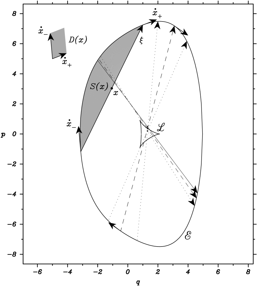
FIG. 1.:

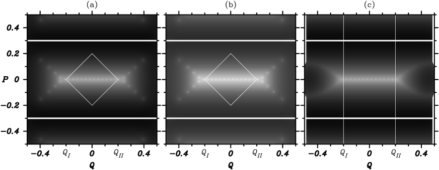
FIG. 2.:

FIG. 3.:

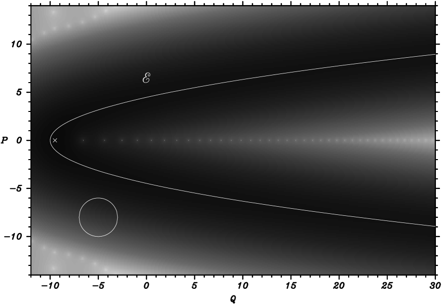
FIG. 4.:

FIG. 5.:

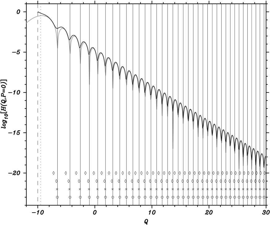
FIG. 6.:

FIG. 7.:

FIG. 8.:

FIG. 9.:

FIG. 10.:

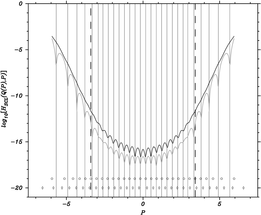
FIG. 11.:

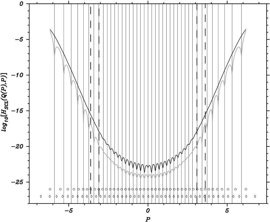
FIG. 12.:

REFERENCES

- [1] M.V.Berry; Phil.Trans.Roy.Soc.287 (1977) 237.
- [2] A.M.Ozorio de Almeida and J.H.Hannay; Ann.Phys. 138 (1982) 115-154.
- [3] A.M.Ozorio de Almeida; Ann.Phys. 145 (1983) 100-114.
- [4] M.V.Berry and N.L.Balazs; J.Phys.A:Math.Gen., 12, No.5 (1979)
- [5] N.L.Balazs; Physica 102A (1980) 236-254.
- [6] N.L.Balazs and B.K.Jennings; Physics Report 104, No.6 (1984) 347-391.
- [7] M.Hillery,R.F.O’Connell,M.O.Scully and E.P.Wigner; Physics Reports 106No.3 (1984) 121-167.
- [8] A.M.Ozorio de Almeida; Physics Reports 295 (1998) 265-342.
- [9] A.Voros; Phy.Rev.A, 40,12 (1989) 6814-6825.
- [10] V.Bargmann; Commun.Pure Appl.Math. XIV (1961) 187.
- [11] A.Perelomov; Generalized Coherent States and their applications, Springer, New York, (1986).
- [12] J.R.Klauder and B.Skagerstam; Coherent States, Applications in Physics and Matehematical Physics, World Scientific, Singapure, (1985).
- [13] K.Husimi; Proc.Phys.Math.Soc.Japan 22 (1940) 264.
- [14] K.Takahashi; J.Physical Soc.Japan 55, No.6 (1986) 762-779.
- [15] J.Kurchan, P Leboeuf and M.Saraceno; Phy.Rev.A, 40,12 (1989) 6800-6813.
- [16] P.Leboeuf and A.Voros; J.Phys.A: Math. Gen.23 (1990) 1765-1774. P.Leboeuf and A.Voros; Quantum nodal as fingerprints of classical chaos, Quantum chaos: between order and disorder: a paper selection compiled and introduced by Gulio Casati, Boris Chirikov. Cambridge University Press (1995).
- [17] M.Abramowitz and I.A.Stegun; Handbook of Mathematical Functions Whashington: US National Bureau of Standards) (1964).
- [18] I.S.Gradshteyn, I.M.Ryzhik; Table of integrals , Series, and Products, Fifth Edition, Academic Press (1994). A.Erdélyi (Bateman Manuscript Project); Higher Transcendental Functions, Vol II, McGraw-Hill (1953).
- [19] C.Cohen Tannoudji, B. Diu, F.Laeoe; Quantum mechanics, Wiley, New York, 1977.
- [20] If the state in (12) is unbounded, the right hand side of (12) changes to . If one of the states in (13) is unbounded, according to the definition of the Wigner function for these kind of states (2), the prefactor needs not be considered; and if the two states are unbounded, the left hand side also changed to .