Thermostating by Deterministic Scattering:
Heat and Shear Flow

Abstract

We apply a recently proposed novel thermostating mechanism to an interacting many-particle system where the bulk particles are moving according to Hamiltonian dynamics. At the boundaries the system is thermalized by deterministic and time-reversible scattering. We show how this scattering mechanism can be related to stochastic boundary conditions. We subsequently simulate nonequilibrium steady states associated to thermal conduction and shear flow for a hard disk fluid. The bulk behavior of the model is studied by comparing the transport coefficients obtained from computer simulations to theoretical results. Furthermore, thermodynamic entropy production and exponential phase-space contraction rates in the stationary nonequilibrium states are calculated showing that in general these quantities do not agree.

PACS numbers: 05.70.Ln, 51.10.+y, 66.20.+d, 66.60.+60

I Introduction

Driving macroscopic systems out of equilibrium requires external forces. Now, the very existence of a nonequilibrium steady state implies that the temperature of the system must remain time independent. One way to prevent the system from heating up indefinitely in nonequilibrium is the introduction of a thermostating algorithm [1]. Starting from molecular dynamics simulations Evans, Hoover, Nosé and others proposed deterministic thermostats to model equilibrium and nonequilibrium fluids [2, 3, 4, 5, 6, 7]. In this formalism the (average) internal energy of the dynamical system is kept constant by subjecting the particles to fictitious frictional forces, thus leading to microcanonical or canonical distributions in phase space [8, 9, 10, 11]. The major feature of this mechanism is its deterministic and time-reversible character, which is in contrast to stochastic thermostats [1, 12, 13, 14, 15, 16]. This allows to elaborate on the connection between microscopic reversibility and macroscopic irreversibility and has led to interesting new links between statistical physics and dynamical systems theory [8, 9, 11, 17], especially to relations between transport coefficients and Lyapunov exponents [18, 19, 20, 21, 22], and between entropy production and phase-space contraction [23, 24, 19, 15, 16, 25, 26, 27, 28]. Although used almost exclusively in the context of nonequilibrium systems, the abovementioned thermostating mechanism presents the drawback that the dynamical equations themselves are altered, even in equilibrium. This raises the question of whether some of the results are due to the special nature of this thermostating formalism or are of general validity [15, 16, 29, 30, 31, 32, 33].

Recently, an alternative mechanism in which thermalization is achieved in a deterministic and time-reversible way has been put forward by Klages et al. [34, 35] and has been applied to a periodic Lorentz gas under an external field. In the present paper we apply this thermostating method to an interacting many-particle system subjected to nonequilibrium boundary conditions giving rise to thermal conduction and to shear flow. The model is closely related to that of Chernov and Lebowitz [15, 16, 36, 37], who study a hard disk fluid driven out of equilibrium into a steady state shear flow by applying special scattering rules at the boundaries in which the particle velocity is kept constant. Our model is introduced in Section II where the thermalization mechanism is tested under equilibrium conditions. In Section III we move on to the case of an imposed temperature gradient and a velocity field by adapting the scattering rules, and we compute the respective transport coefficients. Having a deterministic and time-reversible system at hand we proceed in Section IV to investigate the relation between thermodynamic entropy production and phase-space contraction rate in nonequilibrium stationary states. The main conclusions are drawn in Section V.

II Equilibrium state

Consider a two-dimensional system of hard discs confined in a square box of length $L$ with periodic boundary conditions along the x-axis, i.e., the left and right sides at $x=\pm L/2$ are identified. At the top and bottom sides of the box, $y=\pm L/2$, we introduce rigid walls where the discs are reflected according to certain rules to be defined later. The discs interact among themselves via impulsive hard collisions so that the bulk dynamics is purely conservative. In the following and in all the numerical computations we use reduced units by setting the particle mass $m$, the disk diameter $\sigma$ and the Boltzmann constant $k_{B}$ equal to one.

Before proceeding to the nonequilibrium case we define the disc-wall collision rules in equilibrium and check whether the system is well-behaved. Now, in equilibrium the bulk distribution is Gaussian with a temperature $T$, and the in- and outgoing fluxes at the top and bottom wall have the form (see [12, 13, 14, 15, 16])

$$\Phi(v_{x},v_{y})=(2\pi T^{3})^{-1/2}|v_{y}|\exp\left(-\frac{v_{x}^{2}+v_{y}^{2}}{2T}\right),$$ (1)

with $v_{y}<0$ for the bottom wall and $v_{y}>0$ for the top wall. Imposing stochastic boundary conditions on the systems in this setting would mean that for every incoming particle the outgoing velocities are chosen randomly according to Eq. (1). In practice, this is usually done by drawing numbers from two independent uniformly distributed random generators $\zeta,\xi\in[0,1]$ and then transforming these numbers with the invertible map $\mbox{\boldmath${\cal T}$ }^{-1}:[0,1]\times[0,1]\to[0,\infty)\times[0,\infty)$ as

$$(v_{x},v_{y})=\mbox{\boldmath${\cal T}$ }^{-1}(\zeta,\xi)=\sqrt{2T}\left(\mbox{erf}^{-1}(\zeta),\sqrt{-\ln(\xi)}\right),$$ (2)

which amounts to transforming the uniform densities $\rho(\zeta)=1$ and $\rho(\xi)=1$ onto $\Phi(v_{x},v_{y})$ according to

$$\rho(\zeta)\rho(\xi)\left|\frac{d\zeta d\xi}{dv_{x}dv_{y}}\right|=\left|\frac{\partial\mbox{\boldmath${\cal T}$ }(v_{x},v_{y})}{\partial v_{x}\partial v_{y}}\right|=(2/\pi T^{3})^{1/2}|v_{y}|\exp\left(-\frac{v_{x}^{2}+v_{y}^{2}}{2T}\right).$$ (3)

Note that so far we have restricted Eqs. (2),(3) to positive velocities $v_{x},v_{y}\in[0,\infty)$, which implies a normalization factor in Eq. (3) being different to the one of Eq. (1). In analogy to stochastic boundaries we now define the deterministic scattering at the walls as follows. First, take the incoming velocities $v_{x}$, $v_{y}$ and transform them via $\mbox{\boldmath${\cal T}$ }(v_{x},v_{y})=(\zeta,\xi)$ onto the unit square. Second, use a two-dimensional, invertible, phase-space conserving chaotic map ${\cal M}:[0,1]\times[0,1]\to[0,1]\times[0,1]$ to obtain $(\zeta^{\prime},\xi^{\prime})={\cal M}(\zeta,\xi)$. Finally, transform back to the outgoing velocities via $(v_{x}^{\prime},v_{y}^{\prime})=\mbox{\boldmath${\cal T}$ }^{-1}(\zeta^{\prime},\xi^{\prime})$. In order to render the collision process time-reversible, we also have to distinguish between particles with positive and negative tangential velocities by using ${\cal M}$ and ${\cal M}^{-1}$, respectively. Thus, particles going in with positive (negative) velocities have to go out with positive (negative) velocities and the full collision rules read

$$(v_{x}^{\prime},v_{y}^{\prime}) = \mbox{\boldmath${\cal T}$ }^{-1}\circ{\cal M}\circ\mbox{\boldmath${\cal T}$ }(v_{x},v_{y}),\qquad v_{x}\geq 0$$ (4)

$$(v_{x}^{\prime},v_{y}^{\prime}) = \mbox{\boldmath${\cal T}$ }^{-1}\circ{\cal M}^{-1}\circ\mbox{\boldmath${\cal T}$ }(v_{x},v_{y}),\quad v_{x}<0,$$ (5)

where ${\cal T}$ is meant to be applied to the modulus of the velocities [38]. Since both the positive and the negative side of the tangential velocity distribution of Eq. (1) are normalized to $1/2$, this normalization factor has to be incorporated in Eq.(3) to render the full desired flux $\Phi$ equivalent to the one of Eq. (1). Rewriting Eq. (3) in polar coordinates yields precisely the transformation used in [34, 35], in the limiting case where it mimics a reservoir with infinitely many degrees of freedom. It should also be realized that for obtaining the transformation ${\cal T}$ the total number of degrees of freedom of the reservoir has been projected out onto a single velocity variable, which couples the bulk to the reservoir. Eckmann et al. [39] used a similar idea to go from a Hamiltonian reservoir with infinitely many degrees of freedom to a reduced description when modeling heat transfer via a finite chain of nonlinear oscillators. It remains to assign the form of the chaotic map ${\cal M}$ and we shall first adopt the choice of a baker map, as in Refs. [34, 35],

$$(\zeta^{\prime},\xi^{\prime})={\cal M}(\zeta,\xi)=\left\{\begin{array}[]{l@{\quad;\quad}l}(2\zeta,\xi/2)&0\leq\zeta\leq 1/2\\ (2\zeta-1,(\xi+1)/2)&1/2<\zeta\leq 1\end{array}\right..$$ (6)

Later on we will investigate the consequences of choosing other mappings like the standard map (see, e.g., [40, 41]). Since in equilibrium the in- and outgoing fluxes have the same form as in Eq.(1), the baker map yields a uniform density and our scattering prescription in Eq.(4) can be viewed as a deterministic and time-reversible counterpart of stochastic boundary conditions. ${\cal M}$ being chaotic, the initial and final momentum and energy of any single particle are certainly different, but both quantities should be conserved on the average. The latter is confirmed by numerical experiments in equilibrium, where, as usual in hard disk simulations, we follow a collision-to-collision approach [1]. Keeping the volume fraction occupied by $N=100$ hard disks equal to $\rho=0.1$ sets the length of the box equal to $L=28.0$. After some transient behavior which depends on the temperature of the initial configuration the bulk distribution is Gaussian with zero mean and mean kinetic energy $T/2$ in each directions. The in- and outgoing fluxes at the walls are correctly equipartioned with $T$ as well and have the desired form of Eq.(1), so the system reproduces the correct statistic properties. We close this section by a remark on how we measure the temperature of a flux to or from the boundaries. As the temperature of the tangential component we use the variance of the velocity distribution, $T_{x}:=\left<(v_{x}-\left<v_{x}\right>_{x})^{2}\right>_{x}$, where $<>_{x}$ denotes an average over the density $\rho(v_{x})$. On the other hand, since in the normal direction we actually measure a flux, the appropriate prescription to measure the temperature of this component is $T_{y}:=\left[v_{y}\right]_{y}/\left[v_{y}^{-1}\right]_{y}$, where $[]_{y}$ represents an average over the flux $\Phi$ and the denominator serves as a normalization. The temperatures of the in- and outgoing fluxes at the wall are then defined as $T_{i/o}:=(T_{x}+T_{y})/2$, and $T_{w}:=(T_{i}+T_{o})/2$.

III Nonequilibrium steady state

A Heat flow

1 The Model

In the following, we explicitly indicate the dependence of the transformation ${\cal T}$ on the parameter $T$ by writing $\mbox{\boldmath${\cal T}$ }\!\!_{T}$. This immediately indicates how we may drive our system to thermal nonequilibrium: We just have to use different values of this parameter for the upper ($T^{u}$) and the lower wall ($T^{d}$). We deliberately avoid to use the word ’temperature’ for this parameter, since in contrast to stochastic boundary conditions we have generally no idea how a different $T$ affects the actual temperature of the wall in the sense of the definition given above. In a nonequilibrium situation the temperature of the ingoing flux $\Phi_{i}$ generally does not match exactly the parameter $T$. Therefore, we do not transform onto the uniform invariant density of the baker map anymore, and consequently, the outgoing flux might have all kinds of shapes or temperatures. Nevertheless, the hope is that the mapping ${\cal M}$ will be chaotic enough to smooth out most of the differences and to produce a reasonable outgoing flux $\Phi_{o}$ such that the system is correctly thermostated. And this is indeed what we find in the numerical experiments.

2 Numerical Results

We set $T^{u}=2$, $T^{d}=1$ and $\rho=0.1$ and average over about 40000 particle-particle collisions per particle and about 6000 particle-wall collisions per particle. We divide the available vertical height $L-1$ into 20 equally spaced horizontal layers and calculate the time averages of the number density $n(y)$ of the particles, the mean velocities $u_{x}(y)=\left<v_{x}\right>$, $u_{y}(y)=\left<v_{y}\right>$, and the variances $\left\langle(v_{x}-u_{x})^{2}\right\rangle$, $\left\langle(v_{y}-u_{y})^{2}\right\rangle$. Furthermore, we record the time average of the kinetic energy transfer and measure the temperatures of the in- and outgoing fluxes of both walls as described in the preceding section. The temperatures at the walls are then defined as the mean value of the in- and outgoing temperatures, $T_{w}^{u/d}:=(T_{i}^{u/d}+T_{o}^{u/d})/2$. Time series plots of these quantities confirm the existence of a nonequilibrium stationary state (NSS) induced by the temperature gradient.

Fig. 1 shows the temperature profile between the upper and the lower wall. Apart from boundary effects it is approximately linear, and the respective kinetic energy is equipartitioned between the two degrees of freedom. The parameters $T^{u}$ and $T^{d}$ are represented as (*), and we find a ’temperature’ jump, whereas the measured temperatures $T^{u/d}_{w}$ (+) at the walls seem to continue the bulk profile reasonably well. The profile of the number density $n=4/\pi\rho$ is depicted in Fig. 2. Note again the boundary effects. The densities of the in-coming particles at the upper wall are Gaussian shaped (Figs. 3a,c), whereas the outgoing densities (Figs. 3b,d) show cusps due to the folding property of the baker map. Nevertheless, the baker map produces a reasonable outgoing flux which generates a NSS.

In order to examine the bulk behavior we now compute the thermal conductivity in our computer experiment and compare it to the theoretical value. For this purpose, we measure the heat flux $Q$ across the boundaries and estimate the temperature gradient $dT(y)/dy$ by a linear least square fit to the experimental profile. To discard boundary effects we use only data in the bulk of the system, namely from layer 3 to layer 18, i.e., excluding the top two and the bottom two layers. The experimental heat conductivity is then defined as

$$\lambda_{exp}=Q\left(\frac{dy}{dT}\right),$$ (7)

whereas the theoretical expression for the conductivity of a gas of hard disks with unit mass and unit diameter as predicted by Enskog’s theory reads [42, 43]

$$\lambda_{l}=1.0292\sqrt{\frac{T}{\pi}}\left[\frac{1}{\chi}+\frac{3}{2}bn+0.8718(bn)^{2}\chi\right].$$ (8)

Here, $b$ is the second virial coefficient, $b=\pi/2$, and $\chi$ is the Enskog scaling factor, which is just the pair correlation function in contact[44],

$$\chi=\frac{1-\frac{7}{16}\frac{\pi}{4}n}{(1-\frac{\pi}{4}n)^{2}}.$$ (9)

Since (8) depends on local values of $T$ and $n$ we define the theoretical effective conductivity $\lambda_{th}$ as the harmonic mean over the layers [42],

$$\lambda_{th}=\left(1/N_{layers}\sum_{l=1}^{N_{layers}}1/\lambda_{l}\right)^{-1}.$$ (10)

Table I compares $\lambda_{exp}$ to $\lambda_{th}$ by showing the ratio of the experimental to the theoretical conductivity for different particle numbers and temperature differences. The agreement is quite good, so our thermostating mechanism produces a NSS which is in agreement with hydrodynamics.

Furthermore, going into the hydrodynamic limit by increasing the number of particles we observe that the discontinuity in the outgoing flux of Figs. 3(b,d) diminishes, as expected, since both the in- and outgoing flux come closer to local equilibrium.

B Shear Flow

Inspired by the recently proposed model of Chernov and Lebowitz [15, 16] for a boundary driven planar Couette-flow in a nonequilibrium steady state, we now proceed to check whether it is possible to combine our thermostating mechanism with a positive (negative) drift imposed onto the upper (lower) wall, respectively. Chernov and Lebowitz chose a purely Hamiltonian bulk and simulated the drift at the boundaries by rotating the angle of the particle velocity at the moment of the scattering event with the wall while keeping the absolute value of the velocity constant. This setting could be formulated in a time-reversible way and keeps the total energy of the system generically constant. Here we separate the thermostating mechanism and the drift of the walls by introducing the map

$${\cal S}_{d}(v_{x},v_{y})=(v_{x}+d,v_{y}),$$ (11)

and by applying this shift to the ’thermostated’ velocities. Time-reversibility forces us to do the same before thermostating. Thus, the full particle-wall interaction reads

(Model I) (12)

$$(v_{x}^{\prime},v_{y}^{\prime}) = {\cal S}_{d}\circ\mbox{\boldmath${\cal T}$ }\!\!_{T}^{-1}\circ{\cal M}\circ\mbox{\boldmath${\cal T}$ }\!\!_{T}\circ{\cal S}_{d}(v_{x},v_{y}),\qquad v_{x}\geq-d$$ (13)

$$(v_{x}^{\prime},v_{y}^{\prime}) = {\cal S}_{d}\circ\mbox{\boldmath${\cal T}$ }\!\!_{T}^{-1}\circ{\cal M}^{-1}\circ\mbox{\boldmath${\cal T}$ }\!\!_{T}\circ{\cal S}_{d}(v_{x},v_{y}),\quad v_{x}<-d,$$ (14)

where shifts of different sign are used for the upper (lower) wall to let the walls move into opposite directions. Other prescriptions to impose a shear will be investigated in more detail in the following section.

In the simulations we set $d=\pm 0.05$, $T=T^{u}=T^{d}=1.0$, $N=100$ and $\rho=0.1$. As we expected, we find a NSS with a linear shear profile along the x-direction (Fig. 4), where the drift velocity of the wall $u_{w}$ (*) is defined as the average between the in- and outgoing tangential velocities. The temperature profile is shown in Fig. 5, with the wall temperatures $T_{w}$ (+) defined as above. As can be seen in the plots, none of these values correspond to the parameters $T$ (*) or $d$. Nevertheless, we obtain a linear shear profile $u_{x}(y)$ and an almost quadratic temperature profile $T(y)$, as predicted by hydrodynamics [15].

For a comparison of experimental and theoretical viscosity we follow the same procedure as above, i.e., we estimate the experimental shear rate $du_{x}(y)/dy$ by a linear least square fit $u_{x}(y)=\gamma y$, again discarding the outermost layers. Through the measured momentum transfer from wall to wall $\Pi$ the experimental viscosity is given as

$$\eta_{exp}=\Pi/\gamma,$$ (15)

and the theoretical value as calculated by the Enskog theory has the form [43, 15]

$$\eta_{l}=1.022\frac{1}{2}\sqrt{\frac{T}{\pi}}\left[\frac{1}{\chi}+bn+0.8729(bn)^{2}\chi\right].$$ (16)

Again $b=\pi/2$ denotes the second virial coefficient, $\chi$ is given by Eq.(9) and we use the arithmetic mean of the viscosity over layers 3 - 18 to compute the theoretical viscosity, i.e., $\eta_{th}=1/N_{layers}\sum\eta_{l}$. Table II shows good agreement between the experimental and the theoretical values for different numbers of particles, so again the thermostating mechanism leads to the correct macroscopic behavior. However, the discontinuities in the $v_{x}$-velocity distribution of the scattered particles should be noticed (see Fig.6). This time these discontinuities do not diminish or disappear in the hydrodynamic limit.

IV Entropy production and Phase-Space Contraction

Having a deterministic and reversible dynamics at hand we can now turn to properties beyond the usual hydrodynamic ones and, in particular, investigate the conjectured identity between phase space contraction rate and thermodynamic entropy production in the light of our formalism [23, 24, 19, 15, 16, 25, 26, 27, 28]. In an isolated macroscopic system the entropy is a thermodynamic potential and therefore plays the central role in determining the time evolution and the final equilibrium state. Yet, its microscopic interpretation out of equilibrium remains controversial (see, e.g., [45, 46]) and the situation is even much less clear in NSS. For the class of models where thermostating is ensured by friction coefficients an exact equality between entropy production and phase space contraction rate in NSS has been inferred on the basis of a global balance between the system and the reservoir [23, 8, 9, 11]. For the Chernov-Lebowitz model an approximate equality has also been found [15, 16]. Still, it is not clear under which circumstances this relation holds in general [15, 16, 29, 30, 31, 32, 33].

A Equilibrium State

We begin with the simplest case of equilibrium described in section II, where the thermodynamic entropy production ${\overline{R}}_{eq}$ vanishes. The bulk dynamics being Hamiltonian, phase-space contraction can only occur during collisions with a wall. Since these collisions take place ’ instantaneously’, we ignore the bulk particles and restrict ourselves to the compression related to a single collision during the time interval $dt$. The phase space contraction is then given by the ratio of the one-particle phase-space volume after the collision $(dx^{\prime}dy^{\prime}dv_{x}^{\prime}dv_{y}^{\prime})$ to the one before the collision, $(dxdydv_{x}dv_{y})$, and can thus be obtained from the Jacobi determinant of the scattering process. One easily sees that $dx^{\prime}=dx$ and $|dy^{\prime}/dy|=|v_{y}^{\prime}dt/v_{y}dt|$ [15, 16]. Furthermore,

$$\left|\frac{dv_{x}^{\prime}dv_{y}^{\prime}}{dv_{x}dv_{y}}\right| = \left|\frac{\partial\mbox{\boldmath${\cal T}$ }}{\partial v_{x}\partial v_{y}}\frac{\partial{\cal M}^{(-1)}}{\partial x\partial y}\frac{\partial\mbox{\boldmath${\cal T}$ }^{-1}}{\partial v_{x}^{\prime}\partial v_{y}^{\prime}}\right|=\left|\frac{\partial\mbox{\boldmath${\cal T}$ }}{\partial v_{x}\partial v_{y}}\left[\frac{\partial\mbox{\boldmath${\cal T}$ }}{\partial v_{x}^{\prime}\partial v_{y}^{\prime}}\right]^{-1}\right|$$ (17)

$$= \left|\frac{v_{y}}{v_{y}^{\prime}}\right|\exp\left(\frac{v_{x}^{\prime 2}+v_{y}^{\prime 2}-v_{x}^{2}-v_{y}^{2}}{2T}\right),$$ (18)

where step two follows from the phase-space conservation of ${\cal M}/{\cal M}^{-1}$, and the last line is obtained from Eqs.(2)(3). Hence, in a particle-wall collision the phase-space volume is changed by a factor of

$$\left|\frac{dv_{x}^{\prime}dv_{y}^{\prime}dx^{\prime}dy^{\prime}}{dv_{x}dv_{y}dxdy}\right|=\exp\left(\frac{v_{x}^{\prime 2}+v_{y}^{\prime 2}-v_{x}^{2}-v_{y}^{2}}{2T}\right).$$ (19)

The mean exponential rate of compression of the phase space volume per unit time is thus given by

$$\overline{P}=-<\ln\left|\frac{dv_{x}^{\prime}dv_{y}^{\prime}dx^{\prime}dy^{\prime}}{dv_{x}dv_{y}dxdy}\right|>=\left<(v_{x}^{2}+v_{y}^{2}-v_{x}^{\prime 2}-v_{y}^{\prime 2})/2T\right>,$$ (20)

where the brackets $<>$ denote a time average over all collisions at the top and the bottom walls. In equilibrium the in- and outgoing fluxes associated to these collisions have the same statistical properties, so ${\overline{P}}_{eq}$ sums up to zero and

$${\overline{P}}_{eq}={\overline{R}}_{eq},$$ (21)

This is fully confirmed by the simulations.

B NSS

The thermodynamic entropy production $\sigma$ per unit volume of our system in NSS is given by the Onsager form [15, 8]

$$\sigma(y)=\frac{\Pi}{T}\frac{du_{x}}{dy}+J(y)\frac{d}{dy}\left(\frac{1}{T}\right),$$ (22)

where $\Pi$ is the x-momentum flux in the negative y-direction, and $J(y)$ is the heat flux in the positive y-direction.

1 Heat Flow

Imposing only a temperature gradient on our system like in section III A, the first term in Eq. (22) is identical to zero and the total entropy production $\overline{R}$ in the steady state is then

$$\overline{R}=\int_{Volume}\!\!\!\sigma d{\bf r}=\int_{Surface}\!\!\!J/Tds=J^{u}_{w}/T^{u}_{w}+J^{d}_{w}/T^{d}_{w}$$ (23)

The right hand side of Eq.(23) is the outward entropy flux $J_{w}/T_{w}$ across the walls of the container. Note that there is no temperature slip at the walls with respect to the correctly defined temperature values, as indicated by the simulation results in Figs.1 and 5.

On the other hand, the exponential phase-space contraction rate now reads

$$\overline{P}=\left<(v_{x}^{2}+v_{y}^{2}-v_{x}^{\prime 2}-v_{y}^{\prime 2})/2T_{u}\right>_{u}+\left<(v_{x}^{2}+v_{y}^{2}-v_{x}^{\prime 2}-v_{y}^{\prime 2})/2T_{d}\right>_{d},$$ (24)

where we averaged over the upper and the lower wall separately. Since in NSS $J_{w}^{u}=\left<(v_{x}^{2}+v_{y}^{2}-v_{x}^{\prime 2}-v_{y}^{\prime 2})/2\right>_{u}=-J_{w}^{d}=-\left<(v_{x}^{2}+v_{y}^{2}-v_{x}^{\prime 2}-v_{y}^{\prime 2})/2\right>_{d}$, the ratios of entropy production to exponential phase space contraction rate reduce to

$$\frac{\overline{R}^{u/d}}{\overline{P}^{u/d}}=\frac{T^{u/d}}{T^{u/d}_{w}}.$$ (25)

In the hydrodynamic limit the in- and the outgoing fluxes approach local equilibrium, implying $T_{i}^{u/d}\simeq T_{o}^{u/d}\simeq T_{w}^{u/d}\simeq T^{u/d}$ for both walls. Therefore, the ratios in Eq.(25) should go to unity. The numerical results in Table III confirm this expectation, leading to a good agreement between entropy production and exponential phase-space contraction rate.

2 Shear Flow

We follow the same procedure as in the preceding section. For a stationary shear flow the hydrodynamic entropy production $\sigma$ per unit volume in Eq. (22) can be written as [15, 8]

$$\sigma(y)=\frac{\Pi}{T}\frac{du_{x}}{dy}+J(y)\frac{d}{dy}\left(\frac{1}{T}\right)=\Pi\frac{d}{dy}\left(\frac{u_{x}}{T}\right).$$ (26)

The second step in Eq.(26) follows from the fact that in NSS $\lambda dT/dy=J(y)=\Pi u_{x}(y)$. The total entropy production $\overline{R}$ in the steady shear flow state is then [15, 16]

$$\overline{R}=\int_{Volume}\!\!\!\sigma d{\bf r}=\int_{Surface}\!\!\!\Pi u/Tds$$ (27)

$$=J_{w}/T_{w}=2L^{2}\Pi\left(u_{w}/L\right)/T_{w}=L^{2}\Pi\gamma/T_{w}.$$ (28)

In the macroscopic formulation of irreversible thermodynamics Eq.(27) is interpreted as an equality, in the stationary state, between the entropy produced in the interior and the entropy flow carried across the walls. Our shift map ${\cal S}_{d}$ mimics moving walls with drift velocities $\pm u_{w}$. The work performed at these walls is converted by the viscous bulk into heat and then again absorbed by the walls which now act as infinite thermal reservoirs. By imagining that the walls act as an ’equilibrium’ thermal bath at temperature $T_{w}$, $\overline{R}$ can be interpreted as their entropy increase rate.

For Model I (Eqs.(13)(14)) the mean exponential phase-space contraction rate takes the form ($\partial{\cal S}_{d}/\partial v_{x}\partial v_{y}\equiv 1$)

$$\overline{P}=-\left<[v_{x}^{\prime 2}+v_{y}^{\prime 2}-v_{x}^{2}-v_{y}^{2}-2d(v_{x}^{\prime}+v_{x})]/2T\right>,$$ (29)

whereas the entropy production is given by

$$J_{w}/T_{w}=-\left<[v_{x}^{\prime 2}+v_{y}^{\prime 2}-v_{x}^{2}-v_{y}^{2}-<v_{x}^{\prime}>^{2}+<v_{x}>^{2}]/2T_{w}\right>.$$ (30)

In Table IV the ratios of $L^{2}\Pi\gamma/J_{w}$ as obtained from the simulations are reported and the relation of phase-space contraction rate to entropy production is subsequently checked. Whereas the equality between entropy production and entropy flow via heat transfer is confirmed, we observe a significant difference between entropy production and phase-space contraction which subsists in the hydrodynamic limit. This mismatch is perhaps not so unexpected in view of the distorted outgoing fluxes (see Fig.6). Nevertheless, one could argue that the fine structure of these distributions may depend on the specific characteristics of the baker map chosen to model the collision process. We therefore also considered the standard map

$$\widetilde{\cal M}:\left\{\begin{array}[]{l}\xi^{\prime}=\xi-\frac{k}{2\pi}\sin(2\pi\zeta),\\ \zeta^{\prime}=\zeta+\xi^{\prime},\end{array}\right.$$ (31)

with the parameter $k=100$ to ensure that we are in the hyperbolic regime [40, 41]. We found that the discrepancy between entropy production and phase-space contraction rate remains: although the deterministic map now seems to be chaotic enough to smooth out the fine structure of the outgoing densities, the discontinuity at $d$ survives. Actually, as long as Model I is adopted it becomes clear that in NSS there will always be more out- than ingoing particles with $v_{x}\geq d$ at the upper wall (and with $v_{x}\leq d$ at the lower wall). Thus, the Gaussian halves in Fig.7 (b) will never match to a full Gaussian even in the hydrodynamic limit, and $\Phi_{i}$ and $\Phi_{o}$ will never come close to a local equilibrium. To circumvent this problem we modify the map ${\cal T}$ and investigate the following model:

(Model II) (32)

$$\mbox{\boldmath${\cal T}$ }\!\!_{\pm}(v_{x},v_{y}) = \left(\frac{\mbox{erf}\left[(|v_{x}|\mp d)/\sqrt{2T}\right]\pm\mbox{erf}(d/\sqrt{2T})}{1\pm\mbox{erf}(d/\sqrt{2T})}\,,\exp(-v_{y}^{2}/2T)\right)$$ (33)

$$(v_{x}^{\prime},v_{y}^{\prime}) = \mbox{\boldmath${\cal T}$ }\!\!_{+}^{-1}\circ\widetilde{\cal M}\circ\mbox{\boldmath${\cal T}$ }\!\!_{-}(v_{x},v_{y}),\qquad v_{x}\geq 0$$ (35)

$$(v_{x}^{\prime},v_{y}^{\prime}) = -\mbox{\boldmath${\cal T}$ }\!\!_{-}^{-1}\circ\widetilde{\cal M}^{-1}\circ\mbox{\boldmath${\cal T}$ }\!\!_{+}(v_{x},v_{y}),\quad v_{x}<0.$$ (36)

This model is also time-reversible, but in contrast to the former one no particle changes its tangential direction during the scattering. There is still a gap in the outgoing distribution of Fig.(8) (b), however, simulations show that this gap disappears in the hydrodynamic limit thus bringing the in- and the outgoing distributions close to local equilibrium. Furthermore, we note that whereas we were not able to give a relation between the parameter $d$ and the actual wall velocity $u_{w}$ for Model I, in case of Model II $u_{w}$ converges to $d$ in the hydrodynamic limit. For this reason we chose $d=0.5$ in the following, since this value yields the same order of the wall velocity as $d=0.1$ for Model I. Proceeding now to the phase-space contraction rate we find that it takes the form

$$\overline{P}^{u/d}=-(n_{+}-n_{-})\ln\frac{1\pm\mbox{erf}(d/\sqrt{2T})}{1\mp\mbox{erf}(d/\sqrt{2T})}-\left<[v_{x}^{\prime 2}+v_{y}^{\prime 2}-v_{x}^{2}-v_{y}^{2}-2d(v_{x}^{\prime}+v_{x})]/2T\right>_{u/d}\>,$$ (37)

where $n_{\pm}$ are the collision rates for positive and negative tangential velocities, and the additional term (cf. Eq.(29)) results from the different denominators in Eq.(33). Note that one has to average over the upper and the lower wall separately. Again we compare $\overline{R}$ and $\overline{P}$ (Table V), but although the outgoing flux approaches now a Gaussian in the hydrodynamic limit the two quantities still do not match. This result can be understood in more detail by rearranging the terms in Eq.(37) as

$$\overline{P}^{u/d} = -\left<[v_{x}^{\prime 2}+v_{y}^{\prime 2}-v_{x}^{2}-v_{y}^{2}-<v_{x}^{\prime}>^{2}+<v_{x}>^{2}]/2T\right>_{u/d}$$ (39)

$$-\left<[<v_{x}^{\prime}>^{2}-<v_{x}>^{2}-2d(v_{x}^{\prime}+v_{x})]/2T\right>_{u/d}-(n_{+}-n_{-})\ln\frac{1\pm\mbox{erf}(d/\sqrt{2T})}{1\mp\mbox{erf}(d/\sqrt{2T})}\>.$$

Since $T\to T_{w}$ in the hydrodynamic limit, the first term clearly corresponds to the entropy production Eq.(30). However, the second and the third terms provide additional contributions. For $u_{w}\to d$ and $d\to 0$ they are both of order $d^{2}$ and can be interpreted as a phase space contraction due to a friction parallel to the walls [30]. These two terms apparently depend on the specific modeling of the collision process at the wall. They may physically be interpreted as representing certain properties of a wall, like a roughness, or an anisotropy. Actually, the second term already appeared in Model I, see Eq.(29). The price we had to pay in Model II for the fluxes getting close to local equilibrium is the additional third term in Eq.(39), which does not compensate the second one.

The foregoing analysis shows clearly what to do to get rid of the additional term in Eq.(37): we have to use the same forward and backward transformations $\mbox{\boldmath${\cal T}$ }_{\pm}$ in Eqs.(33,35). If one still wants to transform onto a full Gaussian in the hydrodynamic limit time-reversibility has to be given up. This leads us to propose the model

(Model III) (40)

$$\mbox{\boldmath${\cal T}$ }\!\!_{*}(v_{x},v_{y}) = \left(\frac{\mbox{erf}\left[(v_{x}-d)/\sqrt{2T}\right]+1}{2}\,,\exp(-v_{y}^{2}/2T)\right)$$ (41)

$$(v_{x}^{\prime},v_{y}^{\prime}) = \mbox{\boldmath${\cal T}$ }\!\!_{*}^{-1}\circ\widetilde{\cal M}\circ\mbox{\boldmath${\cal T}$ }\!\!_{*}(v_{x},v_{y}).$$ (43)

which is still deterministic, but no longer time-reversible. The phase-space contraction is now given as

$$\overline{P}=\left<[v_{x}^{\prime 2}+v_{y}^{\prime 2}-v_{x}^{2}-v_{y}^{2}-2d(v_{x}^{\prime}-v_{x})]/2T\right>.$$ (44)

Fig. 9 shows that the in- and the outgoing fluxes are getting close to local equilibrium, implying that the velocity of the wall $u_{w}$ goes to $d$ and the wall temperature $T_{w}$ goes to $T$. Consequently, Eq.(44) should converge to the correct thermodynamic entropy production of Eq.(30) in the hydrodynamic limit, and this is indeed what we observe in Table V. This implies that time-reversibility does not appear to be an essential ingredient for having a relation between phase space contraction and entropy production, as was already stated in Refs. [15, 16, 30]. We remark that we consider the lack of time-reversibility in Model III rather as a technical difficulty of how we define our scattering rules than a fundamental property of this model.

V Conclusion

We have applied a novel thermostating mechanism to an interacting many-particle system. Under this formalism the system is thermalized through scattering at the boundaries while the bulk is left Hamiltonian. We have shown how this deterministic and time-reversible thermostating mechanism is related to conventional stochastic boundary conditions. For a two-dimensional system of hard disks, this thermostat yields a stationary nonequilibrium heat or shear flow state. Transport coefficients obtained from computer simulations, such as thermal conductivity and viscosity, agree with the values obtained from Enskog’s theory.

Having a time-reversible and deterministic system we also examined the relation between microscopic reversibility and macroscopic irreversibility in terms of entropy production. We find that entropy production and exponential phase-space contraction rate do in general not agree. When the NSS is created by a temperature gradient both quantities converge in the hydrodynamic limit. By subjecting the system to a shear we examined three different versions of scattering rules, of which one (Model III) produced an agreement.

Our results indicate that neither time-reversibility nor the existence of a local thermodynamic equilibrium at the walls are sufficient conditions for obtaining an identity between phase space contraction and entropy production. A class of systems where such an identity is guaranteed by default are the ones thermostated by velocity-dependent friction coefficients [8, 9, 11]. We suggest that in general, that is, by using other ways of deterministic and time-reversible thermostating, such an identity may not necessarily exist. We would expect the same to hold for any system where the interaction between bulk and reservoir depends on the details of the microscopic scattering rules.

As a next step it would be important to compute the spectrum of Lyapunov exponents for the models presented in this paper. This would enable to check, for example, the validity of formulas which express transport coefficients in terms of sums of Lyapunov exponents [19, 20], and the existence of a so-called conjugate pairing rule of Lyapunov exponents [20, 36]. Moreover, it would be interesting to verify the fluctuation theorem, as it has been done recently for the Chernov-Lebowitz model [37].

Acknowledgments
Helpful discussions with P.Gaspard, M.Mareschal and K. Rateitschak are gratefully acknowledged. R.K. wants to thank the Deutsche Forschungsgemeinschaft (DFG) for financial support. This work is supported, in part, by the Interuniversity Attraction Pole program of the Belgian Federal Office of Scientific, Technical and Cultural Affairs and by the Training and Mobility Program of the European Commission.

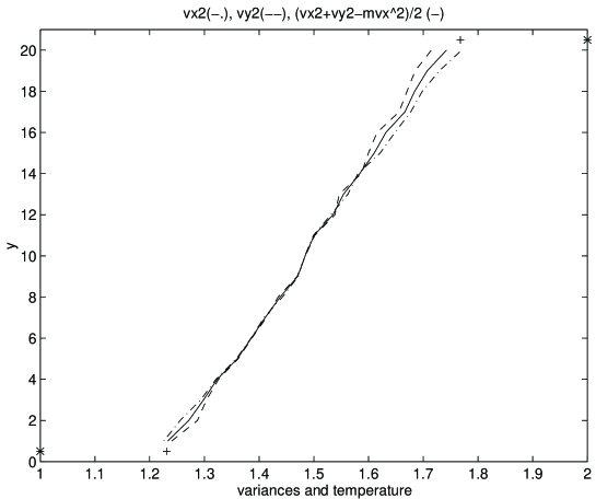
FIG. 1.: Temperature (-) and variance (- -)/(-.) profiles, $T_{u}=2$, $T_{d}=1$ (*). (+) denotes the wall temperatures $T_{w}$ as defined in the text.

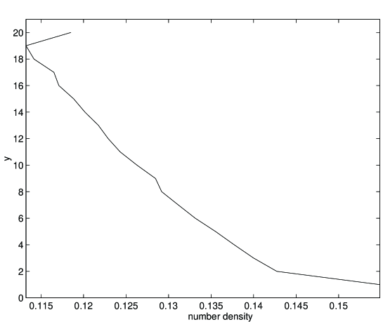
FIG. 2.: The profile of the number density, $T_{u}=2$, $T_{d}=1$ .

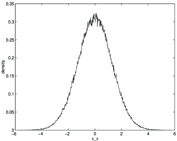
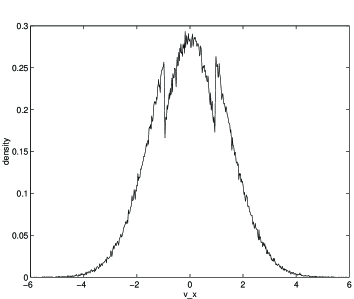
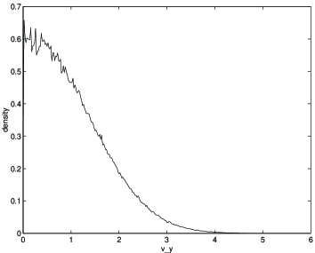
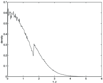
FIG. 3.: Velocity distributions of the in- and outgoing particles at the upper wall ($T=2$) for the heat flow case: a) $v_{x}^{in}$, b) $v_{x}^{out}$, c) $v_{y}^{in}$, d) $v_{y}^{out}$.

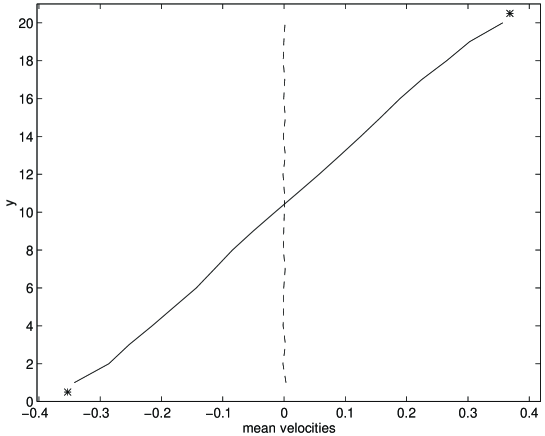
FIG. 4.: Mean velocity in the $x$-direction (–), in the $y$-direction (- -), and at the wall $u_{w}$ (*).

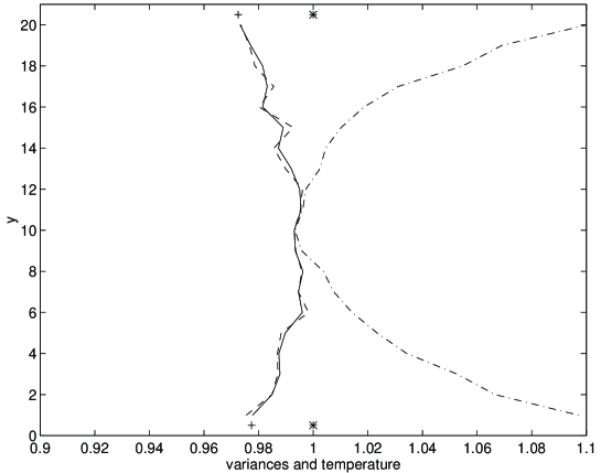
FIG. 5.: Velocity variance in the $x$-direction (- .) and in the $y$-direction (- -), temperature (–), measured wall temperature $T_{w}$ (+) and ’parametrical’ temperature $T$ (*).

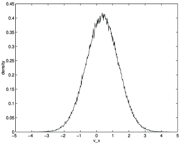
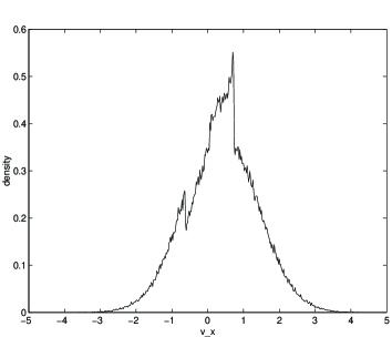
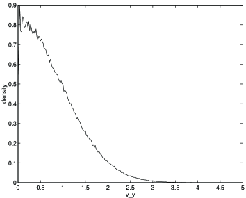
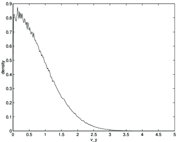
FIG. 6.: Velocity distributions of the in- and outgoing particles at the upper wall for the shear flow case (Model I): a) $v_{x}^{in}$, b) $v_{x}^{out}$, c) $v_{y}^{in}$, d) $v_{y}^{out}$.

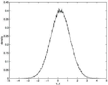
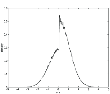
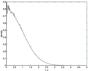
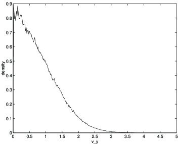
FIG. 7.: Velocity distributions of the in- and outgoing particles at the upper wall for the shear flow case (Model I, standard map): a) $v_{x}^{in}$, b) $v_{x}^{out}$, c) $v_{y}^{in}$, d) $v_{y}^{out}$.

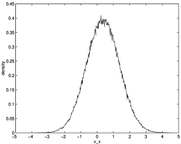
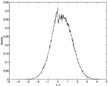
FIG. 8.: Velocity distributions of the in- and outgoing particles at the upper wall for the shear flow case (Model II): a) $v_{x}^{in}$, b) $v_{x}^{out}$.

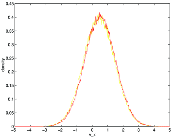
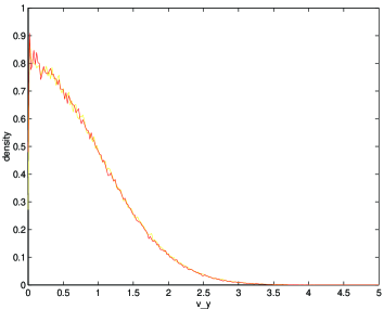
FIG. 9.: Velocity distributions of the in- and outgoing particles at the upper wall for the shear flow case (Model III): a) $v_{x}^{in},v_{x}^{out}$, b) $v_{y}^{in},v_{y}^{out}$.

TABLE I.: Comparison of theoretical and experimental heat conductivity $\lambda_{exp}/\lambda_{th}$

	N=100	N=200	N=400	N=800
$\Delta T$=1.5-1	0.904	1.009	1.003	1.062
$\Delta T$=2.0-1	0.887	0.950	1.021	1.051

TABLE II.: Comparison of theoretical and experimental viscosity $\eta_{exp}/\eta_{th}$

	N=100	N=200	N=400	N=800
$d$=0.05	0.9616	0.9904	1.0081	1.0382
$d$=0.1	0.9702	1.001	1.0226	1.0232

TABLE III.: Comparison of entropy production and exp. phase-space contraction rate $\overline{R}/\overline{P}$, heat flow

	N=100	N=200	N=400	N=800
$T_{u}=1.5$	1.0814	1.0762	1.0614	1.0508
$T_{d}=1$	0.8948	0.9170	0.9273	0.9439
$T_{u}=2$	1.1313	1.1110	1.0985	1.0765
$T_{d}=1$	0.8122	0.8412	0.8633	0.8886

TABLE IV.: Comparison of entropy production and exp. phase-space contraction rate $\overline{R}/\overline{P}$, shear flow, Model I

		N=100	N=200	N=400	N=800
$d$=0.05	$L^{2}\Pi\gamma/J_{w}$	0.9816	0.9669	0.9765	0.9962
baker map	$\overline{R}/\overline{P}$	0.6761	0.5882	0.5023	0.4230
$d$=0.1	$L^{2}\Pi\gamma/J_{w}$	0.9829	0.9664	0.9497	0.9588
baker map	$\overline{R}/\overline{P}$	0.6457	0.5761	0.4934	0.4275
$d$=0.1	$L^{2}\Pi\gamma/J_{w}$	1.0255	1.0424	1.0435	1.0833
standard map	$\overline{R}/\overline{P}$	0.4622	0.3873	0.3008	0.2417

TABLE V.: Comparison of entropy production and exp. phase-space contraction rate $\overline{R}/\overline{P}$, shear flow, Model II and III

		N=100	N=200	N=400	N=800
Model II	$L^{2}\Pi\gamma/J_{w}$	0.9842	1.0154	1.0002	1.0255
$d$=0.5	$\overline{R}/\overline{P}$	0.1858	0.1682	0.1398	0.1127
Model III	$L^{2}\Pi\gamma/J_{w}$	1.0164	1.0046	1.0005	1.0039
$d$=0.5	$\overline{R}/\overline{P}$	0.8452	0.8785	0.9051	0.9619

REFERENCES

- [1] M. Allen and D. Tildesley, Computer simulation of liquids (Clarendon Press, Oxford, 1987).
- [2] D. Evans, J. Chem. Phys. 78, 3297 (1983).
- [3] W. Hoover, A. Ladd, and B. Moran, Phys. Rev. Lett. 48, 1818 (1982).
- [4] D. Evans et al., Phys. Rev. A 28, 1016 (1983).
- [5] S. Nosé, Mol. Phys. 52, 255 (1984).
- [6] S. Nosé, J. Chem. Phys. 81, 511 (1984).
- [7] W. Hoover, Phys. Rev. A 31, 1695 (1985).
- [8] D. Evans and G. Morriss, Statistical Mechanics of Nonequilibrium Liquids, Theoretical Chemistry (Academic Press, London, 1990).
- [9] W. G. Hoover, Computational statistical mechanics (Elsevier, Amsterdam, 1991).
- [10] S. Hess, in Computational physics, edited by K. Hoffmann and M. Schreiber (Springer, Berlin, 1996), pp. 268–293.
- [11] G. Morriss and C. Dettmann, Chaos 8, 321 (1998).
- [12] J. Lebowitz and H. Spohn, J. Stat. Phys. 19, 633 (1978).
- [13] A. Tenenbaum, G. Ciccotti, and R. Gallico, Phys. Rev. A 25, 2778 (1982).
- [14] S. Goldstein, C. Kipnis, and N. Ianiro, J. Stat. Phys. 41, 915 (1985).
- [15] N. Chernov and J. Lebowitz, Phys. Rev. Lett. 75, 2831 (1995).
- [16] N. Chernov and J. Lebowitz, J Statist Phys 86, 953 (1997), 0022-4715.
- [17] J.R. Dorfman, An introduction to chaos in nonequilibrium statistical mechanics (Cambridge University Press, Cambridge, 1999).
- [18] B. Moran and W. Hoover, J. Stat. Phys. 48, 709 (1987).
- [19] H. Posch and W. Hoover, Phys. Rev. A 38, 473 (1988).
- [20] D. Evans, E. Cohen, and G. Morris, Phys. Rev. A 42, 5990 (1990).
- [21] W. N. Vance, Phys. Rev. Lett. 69, 1356 (1992).
- [22] A. Baranyai, D. Evans, and E. Cohen, J. Stat. Phys. 70, 1085 (1993).
- [23] B. L. Holian, W. G. Hoover, and H. A. Posch, Phys. Rev. Lett. 59, 10 (1987).
- [24] H. A. Posch and W. G. Hoover, Phys. Lett. A 123, 227 (1987).
- [25] D. Ruelle, J Statist Phys 85, 1 (1996), 0022-4715.
- [26] D. Ruelle, J Statist Phys 86, 935 (1997), 0022-4715.
- [27] J. Vollmer, T. Tél, and W. Breymann, Phys. Rev. Lett. 79, 2759 (1997).
- [28] W. Breymann, T. Tél, and J. Vollmer, Chaos 8, 396 (1998).
- [29] Microscopic simulations of complex hydrodynamic phenomena, Vol. 292 of NATO ASI Series B: Physics, edited by M. Mareschal and B. L. Holian (Plenum Press, New York, 1992).
- [30] G. Nicolis and D. Daems, Chaos 8, 311 (1998).
- [31] The microscopic approach to complexity in non-equilibrium molecular simulations, Vol. 240 of Physica A, edited by M. Mareschal (Elsevier, Amsterdam, 1997).
- [32] Chaos and Irreversibility, Vol. 8 of Chaos (American Institute of Physics, College Park, 1998).
- [33] P. Gaspard, Chaos, Scattering, and Statistical Mechanics (Cambridge University Press, Cambridge, 1998).
- [34] R. Klages, K. Rateitschak, and G. Nicolis, submitted (unpublished).
- [35] K. Rateitschak, R. Klages, and G. Nicolis (unpublished).
- [36] C. Dellago and H. Posch, J Statist Phys 88, 825 (1997), 0022-4715.
- [37] F. Bonetto, N. I. Chernov, and J. L. Lebowitz, Chaos 8, 823 (1998).
- [38] We note that in our numerical experiments we alternate the application of and in Eq.(4) with respect to the position of the scattering process at the wall to avoid any artificial symmetry breaking.
- [39] J.-P. Eckmann, C.-A. Pillet, and L. Rey-Bellet, chao-dyn/9811001 (unpublished).
- [40] E. Ott, Chaos in Dynamical Systems (Cambridge University Press, Cambridge, 1993).
- [41] J. Meiss, Rev. Mod. Phys. 64, 795 (1992).
- [42] D. Risso and P. Cordero, J. Stat. Phys 82, 1453 (1996).
- [43] D. Gass, J. Chem. Phys. 54, 1898 (1971).
- [44] J. Barker and D. Henderson, Rev. Mod. Phys. 48, 587 (1976).
- [45] J. L. Lebowitz, Physica A 194, 1 (1993).
- [46] J. L. Lebowitz, Phys. Today 46, 32 (1993).