[
STRUCTURAL INVARIANCE AND THE ENERGY SPECTRUM
Abstract
We extend the application of the concept of structural invariance to bounded time independent systems. This concept, previously introduced by two of us to argue that the connection between random matrix theory and quantum systems with a chaotic classical counterpart is in fact largely exact in the semiclassical limit is extended to the energy spectra of bounded time independent systems. We proceed by showing that the results obtained previously for the quasi-energies and eigenphases of the S-matrix can be extended to the eigenphases of the quantum Poincaré map which is unitary in the semiclassical limit. We then show that its eigenphases in the chaotic case move rather stiffly around the unit circle and thus their local statistical fluctuations transfer to the energy spectrum via Bogomolny’s prescription. We verify our results by studying numerically the properties of the eigenphases of the quantum Poincaré map for billiards by using the boundary integral method.
]
I Introduction
In previous papers two of us developed the concept of structural invariance for periodically driven [1] as well as for scattering systems [2, 3] in order to establish the connection between random matrix theory on the one hand and quantum systems with a chaotic classical counterpart on the other. Basically we recovered for such systems the result predicted for the long-range behaviour of the spectral two-point function in a seminal paper by Berry [4] and demonstrated numerically and experimentally in a large, and growing, number of examples [11, 13]: Namely, the fluctuation properties of quantum systems whose classical counterpart is chaotic behave as those of an appropiately chosen ensemble of random matrices. There have been numerous attempts to account for this connection. Among the most notable are periodic orbit theory, which shows how certain random matrix properties arise from a semiclassical formula connecting the density of states with a given sum over periodic orbits. Another approach, which has achieved some remarkable successes recently, is the supersymmetric approach, which has been able to show how such phenomena arise in the context of disordered systems [5]. For chaotic systems without disorder, however, the results obtained in this manner are still far from convincing [6, 7]. The approach taken by structural invariance is in some sense different, since it takes an explicitly probabilistic point of view, asserting only that a chaotic system has RMT properties with probability one and only speaking in terms of ensembles of systems. [1, 14, 8]. This approach has already led to unexpected predictions, which since have been confirmed numerically [9] and later by arguments taken from periodic orbit theory [10].
A weak point of our approach was the fact that its application was in principle restricted to the discussion of eigenphase statistics. In this paper, we shall use the semiclassical quantization of the Poincaré map and its relation to the energy spectrum in order to transfer the statistics of eigenphases to that of eigenvalues. The following relation, due to Bogomolny [20]
| (1) |
shows that we obtain an energy eigenvalue each time one of the eigenphases of the matrix (operator associated to the quantum Poincaré map) takes the value unity; thus a stiff rotation of the unit circle on which the eigenphases are located would transfer their spectral fluctuations to those of the energy eigenvalues. In this paper we shall show that the assumption of fairly uniform speed of the eigenphases as a function of energy is an excellent approximation for chaotic Poincaré maps.
The structure of this paper is as follows: First, in Section 2, we give a short account of structural invariance in the most general terms possible. In Section 3, we review how the connection between classical behaviour and quantum statistics is effected in the case of canonical maps. In Section 4, we proceed to generalize the analysis to Poincaré maps. There we show, using Bogomolny’s semiclassical quantization, that the spectral statistics of the eigenphases of the Poincaré map essentially carry over to those of the eigenvalues. In Section 5, we illustrate the results by means of a numerical computation of the stadium billiard.
II Structural invariance
The point we want to discuss in this Section concerns the construction of a reasonable ensemble given an individual system. Such problems are not really new to physics: indeed, whenever one attempts to describe an individual system by an ensemble, as occurs for example in statistical mechanics, the problem of deriving the ensemble from the individual system arises. In such cases it is well known that one first needs to identify a set of relevant properties. Once this has been done, we define the structural invariance group of the object as the group of all transformations which transform the given object into one with the same relevant properties.
First, let us present a general method to derive such an ensemble. Let us consider a set of objects with given “relevant”properties—the choice of these will turn out to be crucial, though it is usually dictated from the problem at hand—and a specific object taken from this set. Furthermore, let the various objects be transformed among each other through the action of a group . The object has a certain number of the “relevant” properties. We define , the structural invariance group of , in the following manner: Let be that subgroup of which leaves all properties of invariant. If we now act on with all the transformations of , we generate a collection of objects, which has as additional structure that of a homogeneous space under the group . If additionally has an invariant measure, then a measure on can be generated in a natural way as follows: To each subset of one can associate the set of transformations in which map in . The Haar measure of can then be taken as the measure of . This is independent of the choice of , because of the invariance of the Haar measure. Furthermore, it is a measure on that is invariant under the group action and it is therefore clearly singled out.
Let us first consider a trivial example: Consider the set of all infinite binary sequences of ones and minus ones. As relevant properties, we take the value of all finite range correlation functions. By this we mean the following: Consider the sequence . The two-point correlation is then given by
| (2) |
and more general correlations defined through the obvious generalization. As transformations acting on binary sequences, we consider all possible transformations. However, the resulting group is highly pathological and has presumably no Haar measure. One way to proceed is to limit ourselves to large but finite sequences. The group then consists of all transformations mapping arbitrary finite sequences on other arbitrary finite sequences. If the correlations of the original sequence are sufficiently small, then this property is respected by almost all transformations of , that is all but a set of very small measure. The structural invariance group is then the full group. From this follows that we can consider the original sequence as a representative element of the full ensemble of all binary sequences, in which all sequences are taken to be equally probable. On the other hand, if there is a clear predominance of ones, say, but no further correlations, then we can take to be the set of all maps which permute the elements of the original sequence. The set is then the set of all sequences which arise from the original one through permutation, all sequences being equally probable. Again, it is reasonable to assume that the original sequence is indeed a representative member of the ensemble. In this sense, whatever property holds with probability one in the ensemble that has been constructed in this fashion will also presumably hold for the original element. Note that this approach does not always work: For example, if I find a non-zero two-point correlation, it is at least not evident how to define a group that respects this property. A better approach might then be to define a non-invariant measure on that takes this correlation into account and that respects it with probability one. However, it will turn out that we shall be able to define a structural invariance group in the majority of the cases we shall be dealing with.
III Canonical Maps: Asociated Quantum and Classical Ensembles
We now wish to apply the above general approach to the particular case of bijective canonical maps on a compact phase space. To this end, we must define the various ingredients involved in the construction. The set of all objects is the set of all bijective canonical transformations on a compact phase space . The specific object we start from is a given such transformation . As for the “relevant” properties, their choice is dictated by the nature of the problem. In the followoing, we shall principally be interested in the short-range statistical properties of the eigenphases and eigenvalues of the associated unitary and hermitian operators. This corresponds to the long-time properties of the classical time evolution. For this reason, we shall consider only such properties to be “relevant” as remain invariant under arbitrary iteration of the map. As for the group , we shall take it to be the direct product of the group of all bijective canonical canonical transformations with itself, with the following action on the set of all bijective canonical transformations:
| (3) |
To complete the construction, it would be necessary to have a Haar measure on the group . As far as we know, the existence of such a measure has neither been proved nor shown to be impossible. While we believe that such a measure does indeed exist in the case of compact phase spaces, we shall not make siuch an assumption, but rather make the following consideration: After all, what we are really interested in are not the (classical) properties of the canonical maps, but rather those of the corresponding quantum unitary maps. We therefore need to quantize both and the set of all canonical transformations. To this end, we first need to know the quantum equivalent of the phase space . Since is compact, its quantization will be a finite dimensional Hilbert space, with the dimension going to infinity as . Note that in general not all values of yield a quantization of , but only such for which cells of size fit in an integer nuber of times in the phase space . We now proceed to quantize all canonical maps using some quantization technique. Two things shoud be noted here: First, there is no unique way to quantize a canonical map. Second, whichever way is used to associate a unitary map to a canonical map, it can never be such that the quantization of the produvct of two canonical maps is the product of the two quantized maps. Such a result can in deed be obtained, but only approximately, in the limit . After having constructed in the set of all classical maps, we can proceed to define to consist of the set of all unitary maps corresponding to a given quantization of the maps in . In a similar way, we can translate the group in the quantum domain, where it becomes simply , where is the dimension of the Hilbert space. The finiteness of is a crucial point here, and this is precisely the point at which we use the fact that the phase space is compact. From this follows that there exists a (unique) Haar measure on the quantized version of and hence, for every closed subgroup as well.
There is an apparent problem with the above program, however: Since the “translation” from classical to quantum language is by no means unique, one cannot assign to each classical canonical map a well-defined unitary map. Nevertheless, since we are only interested in the semiclassical limit, this problem is not really severe, since all different possible choices will be very close to each other. One might worry, further, that an approximate translation of the group from the classical to the quantum domain might lead one to lose the group property. But this is not the case, since the group is defined through the invariance of the properties of . This definition can itself be carried over to the quantum domain and the group property is then trivially maintained.
Another point that can be raised is the following: Most canonical maps of interest are “simple” or smooth, whereas there is no reason to believe that such smoothness is characteristic of “arbitrary” canonical maps, if this can be given a meaning. Certainly, for unitary maps, it is easy to see that arbitrary unitary maps in a (high-dimensional) Hilbert space representing the semiclassical counterpart of a given classical system with probability one fail to correspond to any reasonable classical canonical transformation. In the light of these facts, one might worry that our reasoning only applies to such systems as are already arbitrarily complex at the classical level, and are therefore inapplicable in the cases of interest, where the map is smooth. We argue that this is incorrect, for the folowing reason: Since we are mainly interested in short-range spectral statistics and since these are dominated by the high iterates of , we are therefore in fact more interested in for than in itself. But is indeed highly irregular, since is chaotic. For this reason, it is presumably qualitatively not different from , where is an “arbitrary” canonical transformation. While such a claim is obviously hard to substantiate, particularly in the absence of a measure on the set of canonical transformations, which would give a precise meaning to the word “arbitrary” in the above phrase, it is very reasonable and intuitively appealing.
A related issue arises with respect to integarble and near-integrable systems: Since sufficiently weak smooth perturbations of an integrable system has invariant tori which cover a non-vanishing measure of phase space, it might appear that the set of all such systems should have positive measure in any ordinary sense of the word, in contradiction to our claim, which is that almost all systems are fully chaotic. This issue is resolved by noting that a generic perturbation in our sense of the word will, in general, not staisfy the smoothness requirements of the KAM theorem, so that any amount of such a generic perturbation will lead to completely irregular dynamics for sufficiently high iterates of the map.
Finally, it remains to see what are the possible special properties of . Since we agree that the only relevant properties are those that remain invariant under arbitrary iterations of the map, we are left with very few possibilities. Here are the three that we are aware of:
—Time-reversal Invariance: If there exists an anti-canonical map (that is, a map which maps the canonical symplectic two-form on its negative) such that and such that
| (4) |
then the map is said to be time-reversal invariant (TRI). In this case, we take to consist of the pairs . These form a group, and it is straightforward to calculate that it leaves the TRI property invariant. As such, it is the structural invariance group of an arbitrary which has no specific property apart from TRI. From this follows that is simply the set of all TRI bijective canonical maps, as was in fact to be expected. On the other hand, we are not (yet!) able to define a measure on , since neither nor have known Haar measures.
This can be readily translated into quantum-mechanical language if we note that in the absence of spin, can be represented as complex conjugation in quantum mechanics, so that is given by the subgroup consisting of the pairs of the type , where is the transpose of .
—Discrete Symmetries: Let commute with a group of canonical transformations . This means that the evolution given by has symmetries, given by the maps . This property is indeed preserved for arbitrary iterations of . The structural invariance group is then given by the subgroup of all pairs such that both and commute with all elements of . Under these circumstances, the action of on respects the property of commuting with and generates as a set the set of all bijective canonical maps that commute with .
Translating into quantum mechanics, this means that the quantum version of consists of all pairs of unitary matrices that commute with the quantization of the maps . This means that the unitary matrices acting to the left and right of can be put in block diagonal form in such a way that each block belongs to a given irreducible representation of . Thus, the ensemble generated has a well defined block structure, in which all blocks statistically independent. On the other hand, if a given block transforms according to a -dimensional representation of , the eigenvalues of the corresponding block will be -fold degenerate.
—Systems with mixed dynamics: A related problem arises with systems having invariant tori, though not, as we shall see, cantori. Indeed, invariant tori are structures which are preserved under arbitrary iterations. Furthermore, at least in the most frequently studied case of two degrees of freedom, they also lead to an absolute division of the phase space in disjoint parts. The structural invariance group should therefore respect these characteristics. The canonical maps belonging to should therefore have the same invariant tori as the map iself. It will therefore automatically also leave the same chaotic regions invariant.
Translating this into quantum mechanics, we see that to each torus there corresponds a unique wave function via the WKB prescription. The above condition therefore means that the group of unitary maps must act on all these integrable eigenfunctions through a phase factor only. From this follows that the eigenphases in this case can be separated in an integrable spectrum, which consists of statistically independent eigenphases—since they are acted upon by the group with its Haar measure—and a chaotic part, which can be treated in the usual way described above, and therefore corresponds to a COE or a CUE for each chaotic region. Note that this follows from the preceding remark: Indeed, when two chaotiic regions are separated by an invariant torus (or an integrable region), the index of the chaotic region is a discrete conserved quantity and acts exactly in the same way as a discrete symmetry.
This leads to various questions concering the relevance of other phase space structures, such as homoclinic and heteroclinic tangles, barriers to transport and cantori. That barriers to transport only define separate phase space regions up to a given number of iterations is clear. For this reason, we should certainly not consider it now, since we are limiting ourselves to the simplest, fully semiclassical case. However, it is clear that such issues will eventually need to be addressed, since structures of this type can notoriously cause strong localization effects. While it is aggreed that these effects are transient when phase space is compact, that is the effects disappear at sufficiently small , they are nevertheless extremely important in practice. Similar arguments allow to rule out the other structures as well: Since they are all invariant sets, it might be argued that they survive under arbitrary iteration. This is true as far as it goes, but they are complex sets, with fractal structure, which quantum mechanics can never fully capture. If we take a finite approximation to such an invariant set, however, it will become ever more complex under iteration and therefore, from the point of view of quantum mechanics, it will eventually become irrelevant.
—Non-primitive Period: It is possible that does not correspond to a primitive period, that is, it might happen that can be written in the form:
| (5) |
for some . In this case, it is not clear to us how to define a structural invariance group that leaves this property invariant, but the remedy is clear enough: It is simpler then to quantize in the first place. The spectral properties of can then be related to those of .
We can now go back to the first two properties, and show that a TRI system will have a COE, whereas a system with a discrete symmetry will have eigenphases thatare divided into statistically independent blocks according to the eigenspaces of . To show the first, we point out that the set consists of all unitary matrices such that
| (6) |
Here denotes the anti-unitary map which represents time reversal in the quantization under consideration. As follows from well-known theorems, it is always possible to choose a basis such that corresponds to complex conjugation. From (6) follows that is a symmetric unitary matrix. The action of the quantum equivalent of on is the following
| (7) |
where denotes the transpose of without complex conjugation. Clearly, this action leaves the symmetry property of invariant. Equally, if we act on by means of for all , we obtain as a set, the set of all symmetric unitary matrices. We are therefore led to ask what measure exists on the set of all symmetric unitary matrices such that it is invariant under the action of given by (7). A standard theorem [12] states that the only such measure is the one known as the Circular Orthogonal Ensemble (COE).
Let us now consider the case of discrete symmetry in some detail, following closely the reasoning presented in [8, 9]. In the case of discrete symmetry, the structural invariance group is given by pairs of unitary matrices acting to the right and to the left of another matrix, which is also block diagonal in the same basis. The Haar measure of is clearly the product measure of the Haar measures of the various unitary groups restriced to each block. From this follows that the ensemble is the product of the various CUE’s involved, which is a well-known empirical fact, as mentioned in the Introduction.
Similarly, we had pointed out a difficulty in the case where the existence of a discrete symmetry was combined with TRI. This can now be treated in the above manner: We must determine the structural invariance group that respects simultaneously TRI and the symmetry . In this case, if we describe everything in a basis adapted to , it is not true any more that we can describe through simple complex conjugation. Define to be the anti-unitary representation of in quantum mechanics. A moment’s thought shows that two cases are possible: First, leaves invariant the eigenspaces belonging to the irreducible representations of . Then, in this eigenspace, can be represented as complex conjugation and the ensemble restricted to this eigenspace is indeed the COE, using the same kind of arguments that lead to the COE when no symmetry is present. On the other hand, can act as the combination of complex conjugation and the operator interchanging the given eigenspace with its time-reversed counterpart. This is clearly only possible if some in is not itself TRI, that is, if
| (8) |
The group is then given by the pairs . In the block diagonal form, the matrix has entries
| (9) |
whereas the matrix gives
| (10) |
From this follows readily that the eigenvalues in both eigenspaces are degenerate, but that the ensemble for each of them is actually the CUE. If we go through the above considerations from the point of view of group theory, we see that this phenomenon can occur whenever some irreducible representation of the symmetry group is not self-adjoint, that is ,when no basis can be found in which all the matrices of the representation are symmetric. The conjugate pair of representations and their associated invariant subspaces will then be interchanged by time-reversal.
This was verified numerically in [9]. The specific example considered was a fully chaotic billiard with threefold symmetry but without any symmetry axis. The rotation by is clearly not TRI and it divides the Hilbert space in three invariant subspaces, generated by for equal to one, zero or minus one modulo three respectively. Whereas the second is clearly invariant under TRI, the other two are interchanged among each other. For these, indeed, GUE statistics was clearly observed, whereas in the TRI subspace the usual GOE was observed. These observations were later confirmed and explained on the basis of periodic orbit theory by Keating and Robbins [10].
IV From eigenphases to eigenvalues
So far we have only treated the case of a bijective canonical map, which can e.g. describe the time evolution of a periodically driven system or a Jung scattering map [15]. An important question, however, is to transfer this analysis to flows generated by a time-independent Hamiltonian. The immediate problem is that we must find a way to account for the fact that the overall density of states is not given by that of the corresponding matrix ensembles and can in fact be rather arbitrary, whereas the fluctuation properties are indeed given by the RMT predictions. This difficulty was absent in the earlier cases since indeed the density of states is correctly predicted to be uniform.
To do this, we consider the energy-dependent Poincaré map , where the variables refer to phase space variables in the Poincaré surface of section. The Poincaré map satisfies the conditions described above: It is bijective (up to a set of points that start from the Poincaré surface but never return to it. By the Poincaré recurrence theorem, however, these are of measure zero and can therefore be disregarded). Further, the part of phase space on which it is defined is a subset of the energy surface, and as such is automatically compact for a bounded system. We therefore deduce that the eigenphases of the Poincaré map are distributed in the way corresponding to the symmetries of the map, which themselves correspond to the symmetries of the system. It now remains to show in which way this distribution of the eigenphases carries over to that of the eigenvalues.
To this end one proceeds as follows: Bogomolny [20] has shown that a semiclassical quantization condition is the following: if is an eigenvalue, then
| (11) |
Thus, if the eigenphases of are denoted by , then every time a given goes through zero, is an eigenvalue. It turns out that the whole procedure is only semiclassical, as the map is only unitary in the semiclassical limit, but this is not a problem, since this limit is in any case the only one we are able to handle. Also, outside of the true semiclassical limit, the relation between chaos and RMT is much more subtle: in particular, one has problems such as (transient) Anderson localization, in which chaotic behaviour and randomly distributed eigenvalues coincide. One also then has to deal with finite tunneling probabilities and other phenomena associated with the structure of our canonical map in the complex plane, which we have left out of consideration entirely, as our understanding of these is still very incomplete.
It therefore appears that we have reduced the problem of determining the spectrum of a Hamiltonian to the study of the energy dependence of the eigenphases of the quantized version of its Poincaré map. Here the tilde indicate canonical variables on the complete phase space, while canonical variables without tilde are defined on the surface of section. To handle the problem, we must first know how the Poincaré map changes under infinitesimal changes of . To this end, let us consider two nearby energies and . The map then maps onto and maps onto a point near to the initial condition. Thus for almost all
| (12) | |||||
| (13) |
where and are small. The exceptions occur if an orbit bifurcates between the two energies and . Since this transformation is canonical, there must exist a “Hamiltonian” , such that
| (14) | |||||
| (15) |
that is
| (16) | |||||
| (17) |
Thus the coordinates on the surface of section satisfy the Hamilton equations for the canonical map where plays the role of the Hamiltonian and plays the role of the time. To show that is the time necessary to return to the Poincaré surface if one starts from we need to use reduced action . By standard arguments[27], is easy to prove that is the generating function of . Using the same arguments, is the generating function of
| (18) |
Finally, the differential of the action of the trajectory that start on and ends on is given by
| (19) |
or
| (20) |
Finally the time to return to the Poincaré surface of section is given by
| (21) |
Summarising the results for the Poincaré map, the infinitesimal canonical transformation close to the identity
| (22) |
means the following: consider the “Hamiltonian” , which is defined as the time necessary to return to the surface of section if one starts from . This “Hamiltonian” generates a flow on the Poincaré surface and is the infinitesimal canonical transformation corresponding to following this flow for a “time” .
If we now follow this through the quantization procedure, we obtain the following: Denote the eigenphases by and be the corresponding eigenfunctions. Thus
| (23) |
If we now denote by the self-adjoint operator corresponding to , we finally obtain
| (24) |
Now we must make some key approximations: First, we remember that we are in the semiclassical limit, that is, that the classical function is smooth compared with the . This implies that instead of using, say, the Wigner distribution in computing the l.h.s. of Eq. (8), we can use a smoothed version such as the Husimi distribution without great error. Since the are eigenfunctions of a matrix representing a totally structureless map, their Husimi distributions will be spread uniformly all over phase space. This would follow from our considerations on structural invariance, but is equally confirmed by a rigorous theorem of Shnirelman’s concerning eigenfunctions of chaotic systems. From this one finally gets
| (25) |
where the overline denotes average over phase space. The crucial points to note is that the right-hand side depends on a classical energy-dependent quantity. However, it is quite independent of the specific wave function and hence of . Since there are eigenphases on the unit circle and they move with a velocity on the order of one, they will cross zero at energies which differ by an order of . This is natural, since we have chosen our scale of energies to be the classical one. Therefore, from one eigenvalue to the next, the velocity at which the eigenphases moves hardly changes. Thus, locally at least, the motion of the eigenphases is quite rigid. This means that the RMT properties of the eigenphases translate directly into corresponding properties of the eigenvalues of the system. On the other hand, it is important to realize that this constancy does not hold forever. Two effects will eventually alter change the velocity: first, the average on the l.h.s. of Eq. (25) will experience a secular change as changes. This corresponds to the secular change in the density of states which is usually eliminated by unfolding the spectrum. On the other hand, another effect may well come into play even before this secular change becomes noticeable. The point is that Eq. (25) is only true as a statistical statement and there are fluctuations around the mean velocity. The most obvious cause for such fluctuations are departures of the Husimi distribution from equidistribution. Such deviations are well-known to exist, namely the so-called “scars” near short periodic orbits. It could therefore well be that these accumulated fluctuations account for some of the effects due to short periodic orbits. To explore this possibility, however, we would presumably require an understanding of scars which we do not have at present. Note also that the long-range stiffness found by Berry [4] is a phenomenon that lies beyond the range of validity of the above remarks. Indeed, its onset is at an infinite distance in terms of the mean level spacing, as we go to the semiclassical limit.
V The quantum Poincaré map on the billiards
Here we will give a numerical example of the principal results of the last section by studying the properties of the eigenphases for the rectangle and Bunimovich sttadium with Neumann boundary conditions. The latter is defined as the (convex) region enclosed by two semicircles of radius connected by two parallel segments of length . This system has been shown [19] to be completely chaotic. Following Bogomolny [20] and Boasman [22], we will use the boundary integral method for the Helmholtz equation. For a billiard defined by a region with boundary it is
| (26) | |||||
| (27) |
where is the normal derivative to the boundary at point . Introducing the usual Green function for the free Laplacian and using the Green identity, on has after integration over the complete region,
| (28) | |||||
| (29) | |||||
| (30) |
where and denote coordinates on the boundary .
Setting and imposing the Neumann boundary conditions (other kind of conditions are straightforward) the last equation takes the form:
| (31) |
Discretising the boundary by equally spaced points and approximating the integral by the trapeze rule, the last equation takes the form
| (32) |
and the eigenvalues of the billiard can be obtained by looking for the roots
| (33) |
when is varied as parameter. Here is the distance introduced by the discretisation of the integral and
| (34) |
The Hankel function is used because in two dimensions
| (35) |
and is the outgoing normal to the boundary at point . To look for the eigenphases we now solve the eigenvalue equation for the matrix .
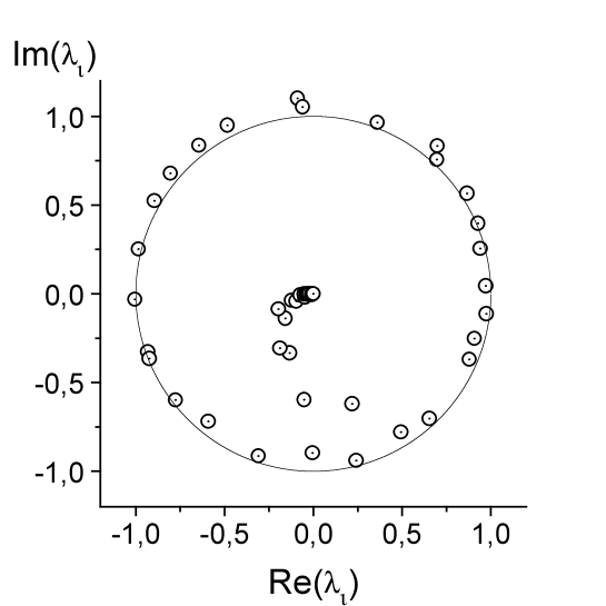
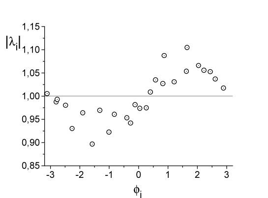
We begin by studying the properties of the eigenphases of the quantum Poincaré map in a rectangle and in a quarter of stadium. The quantum surface of section that we used is the boundary of the billiard. The eigenphases of for a given value of the energy are shown in Fig. 1. The unitarity of the QPM is better in the high energy regime as expected. Also the norms are closer to one when the respective phase is zero or . This behaviour is shown in Fig. 2 where we plotted the norms as function of the phase.
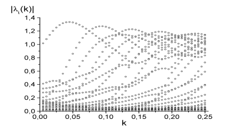
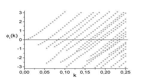
To study in a detailed way the behaviour of the eigenphases of Fig. 1 as functions of the energy we plot in Fig. 3 their phases and norms as function of the energy. This figure suggest that the phases for the stadium move in a “rigid way” when the energy is varied whereas for the rectangle the phases move at least with two velocities. To quantify the velocities we plotted in Fig. 4a the distribution of velocities for the stadium. From this figure is easy to conclude that all eigenphases move basically with the same velocity for the stadium. These results shown the validity of Eq. 25 (this conjecture was also made by Prange [21]) that the eigenvalues in the chaotic case move in a rigid way independently of the number of eigenvalue. This is not the case for the rectangle (integrable system) as we can see in Fig. 4b.
To study the secular variation of eigenphases we plot in Fig. 5 the distributions of the velocities for the stadium for 2 different ranges of . Also, in table I we tabulate the mean values as well as the widths of these and other velocity distributions. From this it is possible to see that these widths are basically constant when is varied in the chaotic case. This is accord with the theoretical prediction of Doron and Smilansky for a behaviour of the width as function of . We also show the widths for integrable systems in table II. It is seen that, for comparable values of the mean, the widths are significantly larger than in the chaotic case. Again, the widths are found to be independent of . The fact that the widts are larger in the integrable case is therefore quite robust under variations of the energy.
The numerical results of this section thus confirm the theoretical predictions: for the completely chaotic case the eigenphases move almost with the same velocity and thus its statistical properties translate to those of the energies. Nevertheless this conclusion does not hold forever. When the eigenvalues have given a complete turn on the unit circle, large correlations must occur. These long range correlations are well known: the saturation in the spectral rigidity (equivalently in the Dyson-Mehta statistics) related to the shortest periodic orbit[4], and the periodicity in the Fourier transform of the two levels cluster function, for Rydberg molecules [26]. Also eigenphases with small velocities have been found in the stadium. These correspond to the bouncing ball states. Note finally that the techniques proposed by Lombardi and coworkers [26] for Rydberg molecules in the framework of Multichannel Quantum Defect Theory can be interpreted from the same point of view and provide an exactly unitary Quantum Poincaré map. These maps dispaly similar properties as those described above for the Poincaré map of the stadium. In particular, the stiffness in the motion of the eigenphases for the case of chaotic motion is also observed in this system [28].
VI Conclusions
We have presented a systematic approach to the connection between RMT and individual dynamical systems. This connection is in a sense of a probabilistic type: it rests basically on conclusions of the form: let a given system be a typical representative of a certain ensemble: If the elements of this ensemble have a given property with probability one, the original system presumably also has the stated property. While this line of argument is wide open to criticisms from the mathematical side, it is undeniably useful at the heuristic level. Further, similar lines of reasoning are frequently used in physics—for example in statistical mechanics—when trying to apply an ensemble description to an individual system. A more genuine concern concerns the construction of the ensembles: as we are not able to construct ensembles on the set of all canonical transformations, we must first construct a set of canonical transformations at the purely classical level and then translate this into quantum mechanics in order to obtain a reasonable candidate for a measure. On the other hand, it may be possible—and we would like to suggest that this would be important—to find an invariant measure on the set of all bijective canonical transformations on a compact phase space. If this were possible, we could define natural classical equivalents to the CUE and the COE. One could then argue in an entirely classical way that a given map with chaotic dynamics is a typical element of such a classical ensemble of canonical maps. Its quantization would therefore belong to the associated quantum ensemble, whence the required spectral properties follow.
Another limitation is the purely semiclassical nature of the analysis. It does not, for example, apply to quantum localization: as long as the phase space is compact, localization is only transient, and therefore outside the immediate range of application of semiclassics. Non-compact phase spaces, on the other hand, also present problems relating to the existence of an invariant measure, not only in the classical, but also in the quantum case.
On the other hand the translation of the fluctuation properties from the eigenphases to the energy spectrum is particularly transparent. Thus the fluctuation properties of the energies are the same as those of the Gaussian ensembles with probability one. This approach shows that not only do the RMT predictions hold for the two-point function at intermediate energy distances, but that they should hold at all energy scales and for all correlation functions. Also the saturation of the long rage stiffness for the energy spectrum is understood in terms of complete turns of the eigenphases on the unit circle. Finally we want to mention that the properties of the velocities of the eigenphases promise to be a new quantum signature of chaos.
VII Acknowledgments
This work is supported by CONACYT-México and by DGAPA-UNAM.
REFERENCES
- [1] F. Leyvraz and T.H. Seligman, Phys. Letts. A 168, 348 (1992)
- [2] T. H. Seligman in Proc. II Wigner Symposium, Goslar 1991, World Scientific Singapore.
- [3] T. H. Seligman in Quantum Chaos, G. Casati and B. V Chirikov, Eds. Cambridge University Press, 1995.
- [4] M.V. Berry, Proc. R. Soc. London A 400, 229 (1985)
- [5] K.B. Efetov, Supersymmetry in Disorder and Chaos, Cambridge University Press (1996)
- [6] A.V. Andreev, O. Agam, B.D. Simons and B.L. Altschuler, Phys. Rev. Lett 76, 3947 (1996)
- [7] F. Leyvraz and T.H. Seligman, Phys. Rev. Lett 79, 1778 (1997)
- [8] F. Leyvraz and T. H. Seligman in Proc. IV Wigner symposium, Guadalajara Mexico, 1995, N. M. Atakishiyev, T. H. Seligman and K. B Wolf (Eds.), World Scientific Singapore.
- [9] F. Leyvraz, C. Schmit and T. H. Seligman, J. Phys. A 29, L575-L580.
- [10] J.P. Keating and J.M. Robbins, J. Phys. A 30, L177 (1997)
- [11] O. Bohigas, M.-J. Giannoni and C. Schmit, Phys. Rev. Lett. 52, 1 (1984); Jour. Physique Letters 45, L1015 (1984)
- [12] E. Cartan, Abh. Math. Seminar Univ. Hamburg, 11, 116 (1935)
- [13] T.H. Seligman and J.J.V. Verbaarschot, Phys. Lett. A 108,183 (1985)
- [14] T. H. Seligman in Jahrbuch 1992/93, Wissenschaftskolleg, Berlin, p. 204 (1994).
- [15] C. Jung and T.H. Seligman, Phys. Rep. 285, 78 (1997)
- [16] M. C. Gutzwiller, Chaos in Classical and Quantum Mechanics Springer Verlag, New-York (1990)
- [17] E. Bogomolny, B. Georgeot, M.-J. Giannoni and C. Schmit, Phys. Rev. Lett. 69, 1477 (1992)
- [18] P. A. M. Dirac, The Principles of Quantum Mechanics, (Oxford University Press, Oxford, 1947)
- [19] L.A. Bunimovich, Comm. in Math. Physics, 65, 295 (1979)
- [20] E. B. Bogomolny, Nonlinearity 5, 805 (1992)
- [21] R. E. Prange, Phys. Rev. Lett. 77, 2447 (1996).
- [22] P. A. Boasman, Nonlinearity 7, 485 (1994)
- [23] J.-P.Eckman and C.-A. Pillet. Preprint chao-dyn9405001.
- [24] A. I. Shnirelman, Usp. Mat. Nauk. 29, 181 (1974).
- [25] M. Moshinsky and C. Quesne. J. Math. Phys. 16, 2017 (1975).
- [26] M. Lombardi and T. H. Seligman. Phys. Rev. A, 29, 3571 (1993).
- [27] L. D. Landau and E. M. Lifshitz. Mechanics, (Pergamon Press, Oxford), 1976.
- [28] R, Méndez, thesis. Also to appear.


| Center | Width | |
|---|---|---|
| 0.02 | 530.586 | 39.839 |
| 0.03 | 528.960 | 39.140 |
| 0.04 | 528.905 | 42.797 |
| 0.05 | 528.826 | 42.575 |
| 0.06 | 529.078 | 39.405 |
| 0.07 | 529.008 | 36.684 |
| 0.08 | 529.788 | 37.352 |
| 0.09 | 530.005 | 33.713 |
| Center | Width | |
|---|---|---|
| 0.02 | 515.438 | 77.142 |
| 0.03 | 516.801 | 85.977 |
| 0.04 | 519.923 | 82.403 |
| 0.05 | 519.559 | 78.797 |
| 0.06 | 520.720 | 73.579 |
| 0.07 | 521.260 | 72.360 |
| 0.08 | 522.025 | 72.095 |
| 0.09 | 522.057 | 71.590 |