Use of Harmonic Inversion Techniques
in Semiclassical Quantization and
Analysis of Quantum Spectra

Abstract

Harmonic inversion is introduced as a powerful tool for both the analysis of quantum spectra and semiclassical periodic orbit quantization. The method allows to circumvent the uncertainty principle of the conventional Fourier transform and to extract dynamical information from quantum spectra which has been unattainable before, such as bifurcations of orbits, the uncovering of hidden ghost orbits in complex phase space, and the direct observation of symmetry breaking effects. The method also solves the fundamental convergence problems in semiclassical periodic orbit theories – for both the Berry-Tabor formula and Gutzwiller’s trace formula – and can therefore be applied as a novel technique for periodic orbit quantization, i.e., to calculate semiclassical eigenenergies from a finite set of classical periodic orbits. The advantage of periodic orbit quantization by harmonic inversion is the universality and wide applicability of the method, which will be demonstrated in this work for various open and bound systems with underlying regular, chaotic, and even mixed classical dynamics. The efficiency of the method is increased, i.e., the number of orbits required for periodic orbit quantization is reduced, when the harmonic inversion technique is generalized to the analysis of cross-correlated periodic orbit sums. The method provides not only the eigenenergies and resonances of systems but also allows the semiclassical calculation of diagonal matrix elements and, e.g., for atoms in external fields, individual non-diagonal transition strengths. Furthermore, it is possible to include higher order terms of the $\hbar$ expanded periodic orbit sum to obtain semiclassical spectra beyond the Gutzwiller and Berry-Tabor approximation.

PACS numbers: 05.45.+b, 03.65.Sq

1 Introduction

1.1 Motivation of semiclassical concepts

Since the development of quantum mechanics in the early decades of this century quantum mechanical methods and computational techniques have become a powerful tool for accurate numerical calculations in atomic and molecular systems. The excellent agreement between experimental measurements and quantum calculations has silenced any serious critics on the fundamental concepts of quantum mechanics, and there are nowadays no doubts that quantum mechanics is the correct theory for microscopic systems. Nevertheless, there has been an increasing interest in semiclassical theories during recent years. The reasons for the resurgence of semiclassics are the following. Firstly, the quantum mechanical methods for solving multidimensional, non-integrable systems generically imply intense numerical calculations, e.g., the diagonalization of a large, but truncated Hamiltonian in a suitably chosen basis. Such calculations provide little insight into the underlying dynamics of the system. By contrast, semiclassical methods open the way to a deeper understanding of the system, and therefore can serve for the interpretation of experimental or numerically calculated quantum mechanical data in physical terms. Secondly, the relation between the quantum mechanics of microscopic systems and the classical mechanics of the macroscopic world is of fundamental interest and importance for a deeper understanding of nature.

This relation was evident in the early days of quantum mechanics, when semiclassical techniques provided the only quantization rules, i.e., the WKB quantization of one-dimensional systems or the generalization to the Einstein-Brillouin-Keller (EBK) quantization [1, 2, 3] for systems with $n$ degrees of freedom. However, the EBK torus quantization is limited to integrable or at least near-integrable systems. In non-integrable systems the KAM tori are destroyed [4, 5], a complete set of classical constants of motion does not exist any more, and therefore the eigenstates of the quantized system cannot be characterized by a complete set of quantum numbers. The “breakdown” of the semiclassical quantization rules for non-regular, i.e., chaotic systems was already recognized by Einstein in 1917 [1]. The failure of the “old” quantum mechanics to describe more complicated systems such as the helium atom [6], and, at the same time, the development and success of the “modern” wave mechanics are the reasons for little interest in semiclassical theories for several decades. The connection between wave mechanics and classical dynamics especially for chaotic systems remained an open question during that period.

1.1.1 Basic semiclassical theories

Chaotic systems: Gutzwiller’s trace formula

The problem was reconsidered by Gutzwiller around 1970 [7, 8]. Although a semiclassical quantization of individual eigenstates is, in principle, impossible for chaotic systems, Gutzwiller derived a semiclassical formula for the density of states as a whole. Starting from the exact quantum expression given as the trace of the Green’s operator he replaced the exact Green’s function with its semiclassical approximation. Applying stationary phase approximations he could finally write the semiclassical density of states as the sum of a smooth part, i.e., the Weyl term, and an oscillating sum over all periodic orbits of the corresponding classical system. For this reason, Gutzwiller’s theory is also commonly known as periodic orbit theory. Gutzwiller’s semiclassical trace formula is valid for isolated and unstable periodic orbits, i.e., for fully chaotic systems with a complete hyperbolic dynamics. Examples of hyperbolic systems are $n$-disk repellers, as models for hyperbolic scattering [9, 10, 11, 12, 13, 14, 15], the stadium billiard [16, 17, 18], the anisotropic Kepler problem [8], and the hydrogen atom in magnetic fields at very high energies far above the ionization threshold [19, 20, 21]. Gutzwiller’s trace formula is exact only in exceptional cases, e.g., for the geodesic flow on a surface with constant negative curvature [8]. In general, the semiclassical periodic orbit sum is just the leading order term of an infinite series in powers of the Planck constant, $\hbar$. Methods to derive the higher order contributions of the $\hbar$ expansion are presented in Refs. [22, 23, 24].

Integrable systems: The Berry-Tabor formula

For integrable systems a semiclassical trace formula was derived by Berry and Tabor [25, 26]. The Berry-Tabor formula describes the density of states in terms of the periodic orbits of the system and is therefore the analogue of Gutzwiller’s trace formula for integrable systems. The equation is known to be formally equivalent to the EBK torus quantization. A generalization of the Berry-Tabor formula to near-integrable systems is given in Refs. [27, 28].

Mixed systems: Uniform semiclassical approximations

Physical systems are usually neither integrable nor exhibit complete hyperbolic dynamics. Generic systems are of mixed type, characterized by the coexistence of regular torus structures and stochastic regions in the classical Poincaré surface of section. A typical example is the hydrogen atom in a magnetic field [29, 30, 31], which undergoes a transition from near-integrable at low energies to complete hyperbolic dynamics at high excitation. In mixed systems the classical trajectories, i.e., the periodic orbits, undergo bifurcations. At bifurcations periodic orbits change their structure and stability properties, new orbits are born, or orbits vanish. A systematic classification of the various types of bifurcations is possible by application of normal form theory [32, 33, 34, 35], where the phase space structure around the bifurcation point is analyzed with the help of classical perturbation theory in local coordinates defined parallel and perpendicular to the periodic orbit. At bifurcation points periodic orbits are neither isolated nor belong to a regular torus in phase space. As a consequence the periodic orbit amplitudes diverge in both semiclassical expressions, Gutzwiller’s trace formula and the Berry-Tabor formula, i.e., both formulae are not valid near bifurcations. The correct semiclassical solutions must simultaneously account for all periodic orbits which participate at the bifurcation, including “ghost” orbits [36, 37] in the complex generalization of phase space, which can be important near bifurcations. Such solutions are called uniform semiclassical approximations and can be constructed by application of catastrophe theory [38, 39] in terms of catastrophe diffraction integrals. Uniform semiclassical approximations have been derived in Refs. [40, 41] for the simplest and generic types of bifurcations and in Refs. [37, 42, 43, 44] for nongeneric bifurcations with higher codimension and corank.

With Gutzwiller’s trace formula for isolated periodic orbits, the Berry-Tabor formula for regular tori, and the uniform semiclassical approximations for orbits near bifurcations we have, in principle, the basic equations for the semiclassical investigation of all systems with regular, chaotic, and mixed regular-chaotic dynamics. There are, however, fundamental problems in practical applications of these equations for the calculation of semiclassical spectra, and the development of techniques to overcome these problems has been the objective of intense research during recent years.

1.1.2 Convergence problems of the semiclassical trace formulae

The most serious problem of Gutzwiller’s trace formula is that for chaotic systems the periodic orbit sum does not converge in the physically interesting energy region, i.e., on and below the real axis, where the eigenstates of bound systems and the resonances of open systems are located, respectively. For chaotic systems the sum of the absolute values of the periodic orbit terms diverges exponentially because of the exponential proliferation of the number of orbits with increasing periods. The convergence problems are similar for the quantization of regular systems with the Berry-Tabor formula, however, the divergence is algebraic instead of exponential in this case.

Because of the technical problems encountered in trying to extract eigenvalues directly from the periodic orbit sum, Gutzwiller’s trace formula has been used in many applications mainly for the interpretation of experimental or theoretical spectra of chaotic systems. For example the periodic orbit theory served as basis for the development of scaled-energy spectroscopy, a method where the classical dynamics of a system is fixed within long-range quantum spectra [45, 46]. The Fourier transforms of the scaled spectra exhibit peaks at positions given by the classical action of the periodic orbits. The action spectra can therefore be interpreted directly in terms of the periodic orbits of the system, and the technique of scaled-energy spectroscopy is now well established, e.g., for investigations of atoms in external fields [47, 48, 49, 50, 51, 52, 53, 54, 55, 56]. The resolution of the Fourier transform action spectra is restricted by the uncertainty principle of the Fourier transform, i.e., the method allows the identification of usually short orbits in the low-dense part of the action spectra. A fully resolved action spectrum would require an infinite length of the original scaled quantum spectrum.

Although periodic orbit theory has been very successful in the interpretation of quantum spectra, the extraction of individual eigenstates and resonances directly from periodic orbit quantization remains of fundamental interest and importance. As mentioned above the semiclassical trace formulae diverge at the physical interesting regions. They are convergent, however, at complex energies with positive imaginary part above a certain value, viz. the entropy barrier. Thus the problem of revealing the semiclassical eigenenergies and resonances is closely related to finding an analytic continuation of the trace formulae to the region at and below the real axis. Several refinements have been introduced in recent years in order to transform the periodic orbit sum in the physical domain of interest to a conditionally convergent series by, e.g., using symbolic dynamics and the cycle expansion [9, 57, 58], the Riemann-Siegel look-alike formula and pseudo-orbit expansions [59, 60, 61], surface of section techniques [62, 63], and heat-kernel regularization [64, 65, 66]. These techniques are mostly designed for systems with special properties, e.g., the cycle expansion requires the existence and knowledge of a symbolic code and is most successful for open systems, while the Riemann-Siegel look-alike formula and the heat-kernel regularization are restricted to bound systems. Until now there is no universal method, which allows periodic orbit quantization of a large variety of bound and open systems with an underlying regular, mixed, or chaotic classical dynamics.

1.2 Objective of this work

The main objective of this work is the development of novel methods for $(a)$ the analysis of quantum spectra and $(b)$ periodic orbit quantization. The conventional action or recurrence spectra obtained by Fourier transformation of finite range quantum spectra suffer from the fundamental resolution problem because of the uncertainty principle of the Fourier transformation. The broadening of recurrence peaks usually prevents the detailed analysis of structures near bifurcations of classical orbits. We will present a method which allows, e.g., the detailed analysis of bifurcations and symmetry breaking and the study of higher order $\hbar$ corrections to the periodic orbit sum. For periodic orbit quantization the aim is the development of a universal method for periodic orbit quantization which does not depend on special properties of the system, such as the existence of a symbolic code or the applicability of a functional equation. As will be shown both problems can be solved by applying methods for high resolution spectral analysis [67]. The computational techniques for high resolution spectral analysis have recently been significantly improved [68, 69, 70], and we will demonstrate that the state of the art methods are a powerful tool for the semiclassical quantization and analysis of dynamical systems.

1.2.1 High precision analysis of quantum spectra

Within the semiclassical approximation of Gutzwiller’s trace formula or the Berry-Tabor formula the density of states of a scaled quantum spectrum is a superposition of sinusoidal modulations as a function of the energy or an appropriate scaling parameter. The frequencies of the modulations are determined by the periods, i.e., the classical action of orbits. The amplitudes and phases of the oscillations depend on the stability properties of the periodic orbits and the Maslov indices. To extract information about the classical dynamics from the quantum spectrum it is therefore quite natural to Fourier transform the spectrum from “energy” domain to “time” (or, for scaled spectra, “action”) domain [45, 46, 47, 71, 72, 73, 74, 75, 76, 77]. The periodic orbits appear as peaks at positions given by the periods of orbits, and the peak heights exhibit the amplitudes of periodic orbit contributions in the semiclassical trace formulae. The comparison with classical calculations allows the interpretation of quantum spectra in terms of the periodic orbits of the corresponding classical system. However, the analyzed experimental or theoretical quantum spectra are usually of finite length, and thus the sinusoidal modulations are truncated when Fourier transformed. The truncation implies a broadening of peaks in the time domain spectra because of the uncertainty principle of the Fourier transform. The widths of the recurrence peaks are determined by the total length of the original spectrum. The uncertainty principle prevents until now precision tests of the semiclassical theories because neither the peak positions (periods of orbits) nor the amplitudes can be obtained from the time domain spectra to high accuracy. Furthermore, the uncertainty principle implies an overlapping of broadened recurrence peaks when the separation of neighboring periods is less than the peak widths. In this case individual periodic orbit contributions cannot be revealed any more. This is especially a disadvantage, e.g., when following, in quantum spectra of systems with mixed regular-chaotic dynamics, the bifurcation tree of periodic orbits. All orbits involved in a bifurcation, including complex “ghost” orbits [36, 37, 44], have nearly the same period close to the bifurcation point. The details of the bifurcations, especially of catastrophes with higher codimension or corank [38, 39], cannot be resolved with the help of the conventional Fourier transform. The same is true for the effects of symmetry breaking, e.g., breaking of the cylindrical symmetry of the hydrogen atom in crossed magnetic and electric fields [54] or the “temporal symmetry breaking” [55, 56] of atoms in oscillating fields. The symmetry breaking should result in a splitting of peaks in the Fourier transform recurrence spectra. Until now this phenomenon could only be observed indirectly via constructive and destructive interference effects of orbits with broken symmetry [54, 55].

To overcome the resolution problem in the conventional recurrence spectra and to achieve a high resolution analysis of quantum spectra it is first of all necessary to mention that the uncertainty principle of the Fourier transformation is not a fundamental restriction to the resolution of the time domain recurrence spectra, and is not comparable to the fundamental Heisenberg uncertainty principle in quantum mechanics. This can be illustrated for the simple example of a sinusoidal function with only one frequency. The knowledge of the signal at only three points is sufficient to recover, although not uniquely, the three unknown parameters, viz. the frequency, amplitude and phase of the modulation. Similarly, a superposition of $N$ sinusoidal functions can be recovered, in principle, from a set of at least $3N$ data points $(t_{i},f_{i})$. If the data points are exact the spectral parameters $\{\omega_{k},A_{k},\phi_{k}\}$ can also be exactly determined from a set of $3N$ nonlinear equations

$$f_{i}=\sum_{k=1}^{N}A_{k}\sin(\omega_{k}t_{i}-\phi_{k})\;,$$ (1.1)

i.e., there is no uncertainty principle. The main difference between this procedure and the Fourier transformation is that we use the linear superposition of sinusoidal functions as an ansatz for the functional form of our data, and the frequencies, amplitudes, and phases are adjusted to obtain the best approximation to the data points. By contrast, the Fourier transform is not based on any constraints. In case of a discrete Fourier transform (DFT) the frequencies are chosen on a (usually equidistant) grid, and the amplitudes are determined from a linear set of equations, which can be solved numerically very efficiently, e.g., by fast Fourier transform (FFT).

As mentioned above the high precision spectral analysis requires the numerical solution of a nonlinear set of equations, and the availability of efficient algorithms has been the bottleneck for practical applications in the past. Several techniques have been developed [67], however, most of them are restricted – for reasons of storage requirements, computational time, and stability of the algorithm – to signals with quite low number of frequencies. By contrast, the number of frequencies (periodic orbits) in quantum spectra of chaotic systems is infinite or at least very large, and applied methods for high precision spectral analysis must be able to handle signals with large numbers of frequencies. This requirement is fulfilled by the method of harmonic inversion by filter-diagonalization, which was recently developed by Wall and Neuhauser [68] and significantly improved by Mandelshtam and Taylor [69, 70]. The decisive step is to recast the nonlinear set of equations as a generalized eigenvalue problem. Using an appropriate basis set the generalized eigenvalue equation is solved with the filter-diagonalization method, which means that the frequencies of the signal can be determined within small frequency windows and only small matrices must be diagonalized numerically even when the signal is composed of a very large number of sinusoidal oscillations.

We will introduce harmonic inversion as a powerful tool for the high precision analysis of quantum spectra, which allows to circumvent the uncertainty principle of the conventional Fourier transform analysis and to extract previously unattainable information from the spectra. In particular the following items are investigated:

• High precision check of semiclassical theories: The analysis of spectra allows a direct quantitative comparison of the quantum and classical periodic orbit quantities to many significant digits.

• Uncovering of periodic orbit bifurcations in quantum spectra, and the verification of ghost orbits and uniform semiclassical approximations.

• Direct observation of symmetry breaking effects.

• Quantitative interpretation of the differences between quantum and semiclassical spectra in terms of the $\hbar$ expansion of the periodic orbit sum.

Results will be presented for various physical systems, e.g., the hydrogen atom in external fields, the circle billiard, and the three disk scattering problem.

1.2.2 Periodic orbit quantization

The analysis of quantum spectra by harmonic inversion and, e.g., the observation of “ghost” orbits, symmetry breaking effects, or higher order $\hbar$ corrections to the periodic orbit contributions provides a deeper understanding of the relation between quantum mechanics and the underlying classical dynamics of the system. However, the inverse procedure, i.e., the calculation of semiclassical eigenenergies and resonances directly from classical input data is of at least the same importance and even more challenging. As mentioned above the periodic orbit sums suffer from fundamental convergence problems in the physically interesting domain and much effort has been undertaken in recent years to overcome these problems [9, 57, 58, 59, 60, 61, 62, 63, 64, 65, 66]. Although many of the refinements which have been introduced are very efficient for a specific model system or a class of systems, they all suffer from the disadvantage of non-universality. The cycle expansion technique [9, 57, 58] requires a completely hyperbolic dynamics and the existence of a symbolic code. The method is most efficient only for open systems, e.g., for three-disk or $n$-disk pinball scattering [9, 10, 11, 12, 13, 14, 15]. By contrast, the Riemann-Siegel look-alike formula and pseudo orbit expansion of Berry and Keating [59, 60, 61] can only be applied for bound systems. The same is true for surface of section techniques [62, 63] and heat-kernel regularization [64, 65, 66]. We will introduce high resolution spectral analysis, and in particular harmonic inversion by filter-diagonalization as a novel and universal method for periodic orbit quantization. Universality means that the method can be applied to open and bound systems with regular and chaotic classical dynamics as well.

Formally the semiclassical density of states (more precisely the semiclassical response function) can be written as the Fourier transform of the periodic orbit recurrence signal

$$C^{\rm sc}(s)=\sum_{\rm po}{\cal A}_{\rm po}\delta(s-s_{\rm po})\;,$$ (1.2)

with ${\cal A}_{\rm po}$ and $s_{\rm po}$ the periodic orbit amplitudes and periods (actions), respectively. If all orbits up to infinite length are considered the Fourier transform of $C^{\rm sc}(s)$ is equivalent to the non-convergent periodic orbit sum. For chaotic systems a numerical search for all periodic orbits is impossible and, furthermore, does not make sense because the periodic orbit sum does not converge anyway. On the other hand, the truncation of the Fourier integral at finite maximum period $s_{\rm max}$ yields a smoothed spectrum only [78]. However, the low resolution property of the spectrum can be interpreted as a consequence of the uncertainty principle of the Fourier transform. We can now argue in an analogous way as in the previous section that the uncertainty principle can be circumvented with the help of high resolution spectral analysis, and propose the following procedure for periodic orbit quantization by harmonic inversion.

Let us assume that the periodic orbits with periods $0<s<s_{\rm max}$ are available and the semiclassical recurrence function $C^{\rm sc}(s)$ has been constructed. This signal can now be harmonically inverted and thus adjusted to the functional form of the quantum recurrence function $C^{\rm qm}(s)$, which is a superposition of sinusoidal oscillations with frequencies given by the quantum mechanical eigenvalues of the system. The frequencies obtained by harmonic inversion of $C^{\rm sc}(s)$ should therefore be the semiclassical approximations to the exact eigenenergies. The universality and wide applicability of this novel quantization scheme follows from the fact that the periodic orbit recurrence signal $C^{\rm sc}(s)$ can be obtained for a large variety of systems because the calculation does not depend on special properties of the system, such as boundness, ergodicity, or the existence of a symbolic dynamics. For systems with underlying regular or chaotic classical dynamics the amplitudes ${\cal A}_{\rm po}$ of periodic orbit contributions are directly obtained from the Berry-Tabor formula [25, 26] and Gutzwiller’s trace formula [8], respectively.

As mentioned above the harmonic inversion technique requires the knowledge of the signal $C^{\rm sc}(s)$ up to a finite maximum period $s_{\rm max}$. The efficiency of the quantization method strongly depends on the signal length which is required to obtain a certain number of eigenenergies. In chaotic systems periodic orbits proliferate exponentially with increasing period and usually the orbits must be searched numerically. It is therefore highly desirable to use the shortest possible signal for periodic orbit quantization. The efficiency of the method can be improved if not just the single signal $C^{\rm sc}(s)$ is harmonically inverted but additional classical information obtained from a set of smooth and linearly independent observables is used to construct a semiclassical cross-correlated periodic orbit signal. The cross-correlation function can be analyzed with a generalized harmonic inversion technique and allows calculating semiclassical eigenenergies from a significantly reduced set of orbits or alternatively to improve the accuracy of spectra obtained with the same set of orbits.

However, the semiclassical eigenenergies deviate – apart from a few exceptions, e.g., the geodesic flow on a surface with constant negative curvature [8] – from the exact quantum mechanical eigenvalues. The reason is that Gutzwiller’s trace formula and the Berry-Tabor formula are only the leading order terms of the $\hbar$ expansion of periodic orbit contributions [22, 23, 24]. It will be shown how the higher order $\hbar$ corrections of the periodic orbit sum can be used within the harmonic inversion procedure to improve, order by order, the semiclassical accuracy of eigenenergies, i.e., to obtain eigenvalues beyond the Gutzwiller and Berry-Tabor approximation.

1.3 Outline

The manuscript is organized as follows. In Chapter 2 the high precision analysis of quantum spectra is discussed. After general remarks on Fourier transform recurrence spectra in Section 2.1 we introduce in Section 2.2 harmonic inversion as a tool to circumvent the uncertainty principle of the conventional Fourier transformation [79]. In Section 2.3 a precision check of the periodic orbit theory is demonstrated by way of example of the hydrogen atom in a magnetic field. For the hydrogen atom in external fields we furthermore illustrate that dynamical information which has been unattainable before can be extracted from the quantum spectra. In Section 2.4 we investigate in detail the quantum manifestations of bifurcations of orbits related to a hyperbolic umbilic catastrophe [44, 80] and a butterfly catastrophe [37, 81], and in Section 2.5 we directly uncover effects of symmetry breaking in the quantum spectra. In Section 2.6 we analyze by way of example of the circle billiard and the three disk system the difference between the exact quantum and the semiclassical spectra. It is shown that the deviations between the spectra can be quantitatively interpreted in terms of the next order $\hbar$ contributions of the $\hbar$ expanded periodic orbit sum.

In Chapter 3 we propose harmonic inversion as a novel technique for periodic orbit quantization [82, 83]. The method is introduced in Section 3.1 for a mathematical model, viz. the calculation of zeros of Riemann’s zeta function. This model shows a formal analogy with the semiclassical trace formulae, and is chosen for the reasons that no extensive numerical periodic orbit search is necessary and the results can be directly compared to the exact zeros of the Riemann zeta function. In Section 3.2 the method is derived for the periodic orbit quantization of physical systems and is demonstrated in Section 3.3 for the example of the three disk scattering system with fully chaotic (hyperbolic) classical dynamics [82, 83], and in Section 3.4 for the hydrogen atom in a magnetic field as a prototype example of a system with mixed regular-chaotic dynamics [84]. In Section 3.5 the efficiency of the method is improved by a generalization of the technique to the harmonic inversion of cross-correlated periodic orbit sums, which allows to significantly reduce the number of orbits required for the semiclassical quantization [85], and in Section 3.6 we derive the concept for periodic orbit quantization beyond the Gutzwiller and Berry-Tabor approximation by harmonic inversion of the $\hbar$ expansion of the periodic orbit sum [86]. The methods of Sections 3.5 and 3.6 are illustrated in Section 3.7 for the example of the circle billiard [85, 86, 87, 88]. Finally, in Section 3.8 we demonstrate the semiclassical calculation of individual transition matrix elements for atoms in external fields [89].

Chapter 4 concludes with a summary and outlines possible future applications, e.g., the analysis of experimental spectra and the periodic orbit quantization of systems without scaling properties.

Computational details of harmonic inversion by filter-diagonalization are presented in Appendix A, and the calculation and asymptotic behavior of some catastrophe diffraction integrals is discussed in Appendix C.

2 High precision analysis of quantum spectra

Semiclassical periodic orbit theory [7, 8] and closed orbit theory [90, 91, 92, 93] have become the key for the interpretation of quantum spectra of classically chaotic systems. The semiclassical spectra at least in low resolution are given as the sum of a smooth background and a superposition of modulations whose amplitudes, frequencies, and phases are solely determined by the closed or periodic orbits of the classical system. For the interpretation of quantum spectra in terms of classical orbits it is therefore most natural to obtain the recurrence spectrum by Fourier transforming the energy spectrum to the time domain. Each closed or periodic orbit should show up as a sharp $\delta$-peak at the recurrence time (period), provided, first, the classical recurrence times do not change within the whole range of the spectrum and, second, the Fourier integral is calculated along an infinite energy range. Both conditions are usually not fulfilled. However, the problem regarding the energy dependence of recurrence times can be solved in systems possessing a classical scaling property by application of scaling techniques. The second condition is never fulfilled in practice, i.e., the length of quantum spectra is always restricted either by experimental limitations or, in theoretical calculations, by the growing dimension of the Hamiltonian matrix which has to be diagonalized numerically. The given length of a quantum spectrum determines the resolution of the quantum recurrence spectrum due to the uncertainty principle, $\Delta E\cdot\Delta T\sim\hbar$, when the conventional Fourier transform is used. Only those closed or periodic orbits can be clearly identified quantum mechanically which appear as isolated non-overlapping peaks in the quantum recurrence spectra. This is especially not the case for orbits which undergo bifurcations at energies close to the bifurcation point. As will be shown the resolution of quantum recurrence spectra can be significantly improved beyond the limitations of the uncertainty principle of the Fourier transform by methods of high resolution spectral analysis.

In the following we first review the conventional analysis of quantum spectra by Fourier transformation and discuss on the example of the hydrogen atom in a magnetic field the achievements and limitations of the Fourier transform recurrence spectra. In Section 2.2 we review methods of high resolution spectral analysis which can serve to circumvent the uncertainty principle of the Fourier transform. In Sections 2.3 to 2.6 the harmonic inversion technique is applied to calculate high resolution recurrence spectra beyond the limitations of the uncertainty principle of the Fourier transformation from experimental or theoretical quantum spectra of finite length. The method allows to reveal information about the dynamics of the system which is completely hidden in the Fourier transform recurrence spectra. In particular, it allows to identify real orbits with nearly degenerate periods, to detect complex “ghost” orbits which are of importance in the vicinity of bifurcations [36, 37, 44], and to investigate higher order $\hbar$ corrections of the periodic orbit contributions [22, 23, 24].

2.1 Fourier transform recurrence spectra

According to periodic orbit theory [7, 8] the semiclassical density of states can be written as the sum of a smooth background $\varrho_{0}(E)$ and oscillatory modulations induced by the periodic orbits,

$$\varrho(E)=\varrho_{0}(E)+{1\over\pi}{\rm Re}\,\sum_{\rm po}\sum_{r=1}^{\infty}A_{\rm po,r}(E)e^{irS_{\rm po}(E)/\hbar}\;,$$ (2.1)

with $A_{\rm po,r}(E)$ the amplitudes of the modulations and the classical actions $S_{\rm po}(E)$ of a primitive periodic orbit (po) determining the frequencies of the oscillations. Linearizing the action around $E=E_{0}$ yields

$$S(E)\approx S(E_{0})+\left.{dS\over dE}\right|_{E_{0}}(E-E_{0})=S(E_{0})+T_{0}(E-E_{0})\;,$$ (2.2)

with $T_{0}$ the time period of the orbit at energy $E_{0}$. When Eq. (2.2) is inserted in (2.1) the semiclassical density of states is locally given as a superposition of sinusoidal oscillations, and it might appear that the problem of identifying the amplitudes $A_{\rm po}$ and time periods $T_{\rm po}$ that contribute to the quantum spectrum $\varrho(E)$ can be solved by Fourier transforming $\varrho(E)$ to the time domain, i.e., each periodic orbit should show up as a $\delta$-peak at the recurrence time $t=T_{0}$. However, fully resolved recurrence spectra can be obtained only if the two following conditions are fulfilled. First, the Fourier integral is calculated along an infinite energy range, and, second, the classical recurrence times do not change within the whole range of the spectrum. The first condition is usually not fulfilled when quantum spectra are obtained from an experimental measurement or a numerical quantum calculation. In that case the Fourier transformation is restricted to a finite energy range and the resolution of the time domain spectrum is limited by the uncertainty principle of the Fourier transform. It is the main objective of this Chapter to introduce high resolution methods for the spectral analysis which allow to circumvent the uncertainty principle of the Fourier transform and to obtain fully resolved recurrence spectra from the analysis of quantum spectra with finite length. However, the second condition is usually not fulfilled either. Both the amplitudes and recurrence times of periodic orbits are in general nontrivial functions of the energy $E$, and, even worse, the whole phase space structure changes with energy when periodic orbits undergo bifurcations. For the interpretation of quantum spectra in terms of periodic orbit quantities it is therefore in general not appropriate to analyze the frequencies of long ranged spectra $\varrho(E)$. The problems due to the energy dependence of periodic orbit quantities have been solved by the development and application of scaling techniques.

Scaling techniques

Many systems possess a classical scaling property in that the classical dynamics does not depend on an external scaling parameter $w$ and the action of trajectories varies linearly with $w$. Examples are systems with homogeneous potentials, billiard systems, or the hydrogen atom in external fields. In billiard systems the shapes of periodic orbits are solely determined by the geometry of the borders, and the classical action depends on the length $L_{\rm po}$ of the periodic orbit, $S_{\rm po}=\hbar kL_{\rm po}$, with $k$ the wave number. For a particle with mass $m$ moving in a billiard system it is therefore most appropriate to take the wave number as the scaling parameter, i.e., $w=k=\sqrt{2mE}/\hbar$. For a system with a homogeneous potential $V({\bf q})$ with $V(c{\bf q})=c^{\alpha}V({\bf q})$ only the size of periodic orbits but not their shape changes with varying energy $E$. Introducing a scaling parameter as a power of the energy, $w=E^{1/\alpha+1/2}$, the classical action of a periodic orbit is obtained as $S_{\rm po}(E)=(E/E_{0})^{1/\alpha+1/2}S_{\rm po}(E_{0})$, with $E_{0}$ being a reference energy, i.e., the action depends linearly on a scaling parameter defined as $w=(E/E_{0})^{1/\alpha+1/2}$. For example the Coulomb potential is a homogeneous potential with $\alpha=-1$ and the bound Coulomb spectrum at negative energies ($E_{0}=-1/2$) is transformed by the scaling procedure to a simple spectrum with equidistant lines at $w=n$ with $n=1,2,\dots$ the principal quantum number. For atoms in external magnetic and electric fields the shape of periodic orbits changes if the field strengths are fixed and only the energy is varied. However, these systems possess a scaling property if both the energy and the field strengths are simultaneously varied. Details for the hydrogen atom in a magnetic field will be given below. The scaling parameter plays the role of an inverse effective Planck constant, $w=\hbar_{\rm eff}^{-1}$. In theoretical investigations it is even possible to apply scaling techniques to general systems with non-homogeneous potentials if the Planck constant is formally used as a variable parameter. Non-homogeneous potentials are important, e.g., in molecular dynamics, and the genaralized scaling technique has been applied in Ref. [94] to analyze quantum spectra of the HO₂ molecule.

When the scaling technique is applied to a quantum system the scaling parameter $w$ is quantized, i.e., bound systems exhibit sharp lines at real eigenvalues $w=w_{k}$ and open systems have resonances related to complex poles $w=w_{k}$ of the scaled Green’s function $G^{+}(w)$. By varying the scaled energy a direct comparison of the quantum recurrence spectra with the bifurcation diagram of the underlying classical system is possible [45, 47].

The semiclassical approximation to the scaled spectrum is given by

$$\varrho(w)=\varrho_{0}(w)+{1\over\pi}{\rm Re}\,\sum_{\rm po}\sum_{r=1}^{\infty}A_{\rm po,r}e^{irs_{\rm po}w}\;,$$ (2.3)

with

$$s_{\rm po}=\oint_{\rm po}{\tilde{\bf p}}d{\tilde{\bf q}}={1\over w}\oint_{\rm po}{\bf p}d{\bf q}$$ (2.4)

the scaled action of a primitive periodic orbit. The vectors $\tilde{\bf q}$ and $\tilde{\bf p}$ are the coordinates and momenta of the scaled Hamiltonian. In contrast to Eq. 2.1 the periodic orbit sum (2.3) is a superposition of sinusoidal oscillations as a function of the scaling parameter $w$. Therefore the scaled spectra $\varrho(w)$ can be Fourier transformed along arbitrarily long ranges of $w$ to generate Fourier transform recurrence spectra of in principle arbitrarily high resolution, i.e., yielding sharp $\delta$-peaks at the positions of the scaled action $s=s_{\rm po}$ of periodic orbits. The high resolution analysis of quantum spectra in the following sections is possible only in conjunction with the application of the scaling technique.

The periodic orbit amplitudes $A_{\rm po,r}$ in Gutzwiller’s trace formula (2.3) for scaled systems are given by

$$A_{\rm po,r}={s_{\rm po}\over\sqrt{|{\rm det}(M_{\rm po}^{r}-I)|}}\,e^{-ir{\pi\over 2}\mu_{\rm po}}\;,$$ (2.5)

with $M_{\rm po}$ and $\mu_{\rm po}$ the monodromy matrix and Maslov index of the primitive periodic orbits, respectively, and $r$ the repetition number of orbits. The monodromy matrix ${\bf M}$ is the stability matrix restricted to deviations perpendicular to a periodic orbit after period time $T$. We here discuss systems with two degrees of freedom. If $\delta q(0)$ is a small deviation perpendicular to the orbit in coordinate space at time $t=0$ and $\delta p(0)$ an initial deviation in momentum space, the corresponding deviations at time $t=T$ are related to the monodromy matrix [93, 95]:

$$\left(\begin{array}[]{c}\delta q(T)\\ \delta p(T)\end{array}\right)={\bf M}\left(\begin{array}[]{c}\delta q(0)\\ \delta p(0)\end{array}\right)=\left(\begin{array}[]{c}m_{11}~{}m_{12}\\ m_{21}~{}m_{22}\end{array}\right)\left(\begin{array}[]{c}\delta q(0)\\ \delta p(0)\end{array}\right)\;.$$ (2.6)

To compute ${\bf M}$ one considers an initial deviation solely in coordinate space to obtain the matrix elements $m_{11}$ and $m_{21}$, and an initial deviation solely in momentum space to obtain $m_{12}$ and $m_{22}$. In practice a linearized system of differential equations obtained by differentiating Hamilton’s equations of motion with respect to the phase space coordinates is numerically integrated. The Maslov index $\mu_{\rm po}$ increases by one every time the trajectory passes a conjugate point or a caustic. Therefore the amplitudes $A_{\rm po,r}$ are complex numbers containing phase information determined by the Maslov indices of orbits. The classical actions $s_{\rm po}$ are usually real numbers, although they can be complex in general. Non-real actions $s_{\rm po}$ indicate “ghost” orbits [36, 37, 44] which exist in the complex continuation of the classical phase space.

As mentioned above the problem of identifying $A_{\rm po}$ and $s_{\rm po}$ that contribute to the quantum spectrum $\varrho(w)$ can in principle be solved by Fourier transforming $\varrho(w)$ to the action domain,

$$C(s)={1\over 2\pi}\int_{w_{1}}^{w_{2}}\left[\varrho(w)-\varrho_{0}(w)\right]e^{-isw}dw\;.$$ (2.7)

If the quantum spectrum $\varrho(w)$ has infinite length and the periodic orbits (i.e., the actions $s_{\rm po}$) are real the Fourier transform of Eq. 2.3 indeed results in a fully resolved recurrence spectrum

$$C(s) = {1\over 2\pi}\int_{-\infty}^{+\infty}\left[\varrho(w)-\varrho_{0}(w)\right]e^{-isw}dw$$ (2.8)

$$= {1\over 2\pi}\sum_{\rm po}\sum_{r=1}^{\infty}\left(A_{\rm po,r}\delta(s-rs_{\rm po})+A_{\rm po,r}^{\ast}\delta(s+rs_{\rm po})\right)\;.$$

The periodic orbits are identified as $\delta$-peaks in the recurrence spectrum at positions $s=\pm s_{\rm po}$ (and their repetitions at $s=\pm rs_{\rm po}$) and the recurrence strengths are given as the amplitudes $A_{\rm po,r}$ (Eq. 2.5) of Gutzwiller’s trace formula. However, for finite range spectra the $\delta$-functions in Eq. 2.8 must be replaced apart from a phase factor with

$$\delta(s)\longrightarrow{\sin((w_{2}-w_{1})s/2)\over\pi s}\;.$$

Unfortunately, the recurrence peaks are broadened by the uncertainty principle of the Fourier transform and furthermore the function $\sin((w_{2}-w_{1})s/2)/\pi s$ has side-peaks which are not related to recurrences of periodic orbits but are solely an undesirable effect of the sharp cut of the Fourier integral at $w_{1}$ and $w_{2}$. In complicated recurrence spectra it can be difficult or impossible to separate the physical recurrences and the unphysical side-peaks. The occurrence of side-peaks can be avoided by multiplying the spectra with a window function $h(w)$, i.e.

$$C(s)={1\over 2\pi}\int_{w_{1}}^{w_{2}}h(w)\left[\varrho(w)-\varrho_{0}(w)\right]e^{-isw}dw\;,$$ (2.9)

where $h(w)$ is equal to one at the center of the spectrum and decreases smoothly close to zero at the borders $w_{1}$ and $w_{2}$ of the Fourier integral. An example is a Gaussian window

$$h(w)=\exp\left(-{(w-w_{0})^{2}\over 2\sigma^{2}}\right)$$

centered at $w_{0}=(w_{1}+w_{2})/2$ and with sufficiently chosen width $\sigma\approx(w_{2}-w_{1})/6$. The Gaussian window suppresses unphysical side-peaks in the recurrence spectra, however, the decrease of the side-peaks is paid by an additional broadening of the central peak. Various other types of window functions $h(w)$ have been used as a compromise between the least uncertainty of the central recurrence peak and the optimal suppression of side-peaks. However, the fundamental problem of the uncertainty principle of the Fourier transform cannot be solved with any window function $h(w)$.

As a first example for the analysis of quantum spectra we introduce the hydrogen atom in a magnetic field (for reviews see [29, 30, 31]) given by the Hamiltonian [in atomic units, magnetic field strength $\gamma=B/(2.35\times 10^{5}\,{\rm T})$, angular momentum $L_{z}=0$]

$$H={1\over 2}{\bf p}^{2}-{1\over r}+{1\over 8}\gamma^{2}(x^{2}+y^{2})\;.$$ (2.10)

As mentioned above this system possesses a scaling property. Introducing scaled coordinates, $\tilde{\bf r}=\gamma^{2/3}{\bf r}$, and momenta, $\tilde{\bf p}=\gamma^{-1/3}{\bf p}$, the classical dynamics of the scaled Hamiltonian

$$\tilde{H}={1\over 2}\tilde{\bf p}^{2}-{1\over\tilde{r}}+{1\over 8}(\tilde{x}^{2}+\tilde{y}^{2})=E\gamma^{-2/3}\;.$$ (2.11)

does not depend on two parameters, the energy $E$ and the magnetic field strength $\gamma$, but solely on the scaled energy

$$\tilde{E}=E\gamma^{-2/3}\;.$$ (2.12)

The classical action of the trajectories scales as

$$S_{\rm po}=s_{\rm po}\gamma^{-1/3}=s_{\rm po}w\;.$$ (2.13)

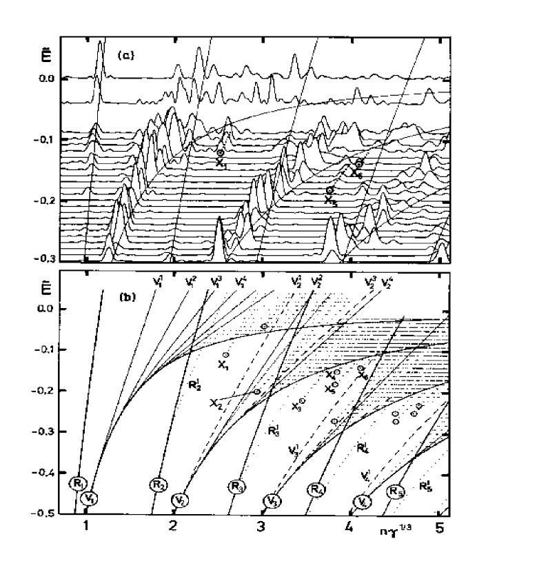
Figure 1: (a) Experimental recurrence spectra of the hydrogen atom in a magnetic field in overlay form. Even-parity, $m=0$ final state. (b) Scaled action of closed classical orbits through origin. (From Ref. [45].)

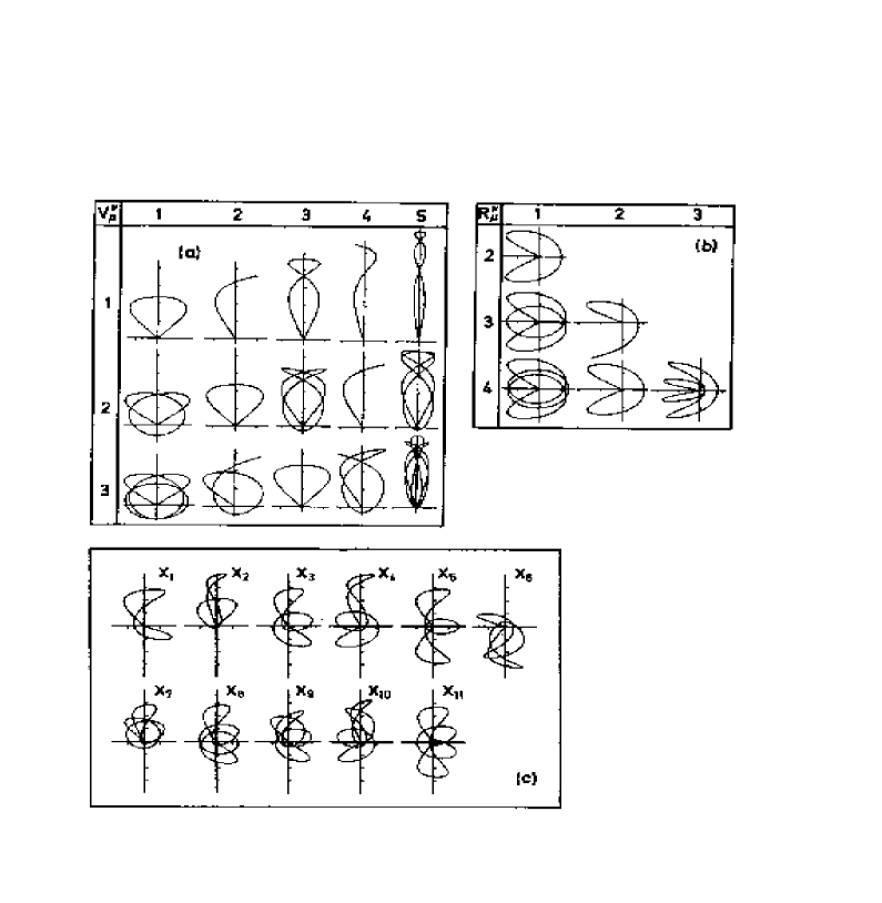
Figure 2: Closed classical orbits of the hydrogen atom in a magnetic field in $(\rho,z)$ projection. (a) Vibrator, (b) rotator, and (c) “exotic” orbits. (From Ref. [46].)

Based on the scaling relations of the classical Hamiltonian the experimental technique of scaled energy spectroscopy was developed [45, 46, 47]. Experimental spectra on the hydrogen atom at constant scaled energy have been measured by varying the magnetic field strength linearly on a scale $w\equiv\gamma^{-1/3}$, adjusting simultaneously the energy $E$ (via the wave length of the exciting laser light) so that the scaled energy $\tilde{E}=E\gamma^{-2/3}$ is kept constant at a given value. The spectra have been Fourier transformed in the experimentally accessible range $36\leq\gamma^{-1/3}\leq 50$. Experimental recurrence spectra at scaled energies $-0.3\leq\tilde{E}\leq 0$ are presented in Fig. 1a. The overlay exhibits a well-structured system of clustered branches of resonances in the scaled energy-action plane. For comparison Fig. 1b presents the energy-action spectrum of the closed classical orbits, i.e. the scaled action of orbits as a function of the energy. As can be seen the clustered branches of resonances in the experimental recurrence spectra (Fig. 1a) well resemble the classical bifurcation tree of closed orbits in Fig. 1b, although a one to one comparison between recurrence peaks and closed orbits is limited by the finite resolution of the quantum recurrence spectra. Closed orbits bifurcating from the $\mu$th repetition of the orbit parallel to the magnetic field axis are called “vibrators” $V_{\mu}^{\nu}$, and orbits bifurcating from the $\mu$th repetition of the perpendicular orbit are called “rotators” $R_{\mu}^{\nu}$ in Fig. 1. Orbits $X_{\mu}$ are created mainly in tangent bifurcations. The graphs of some closed orbits are given in Fig. 2. A detailed comparison of the peak heights of resonances in the experimental recurrence spectra with the semiclassical amplitudes obtained from closed orbit theory can be found in Ref. [47].

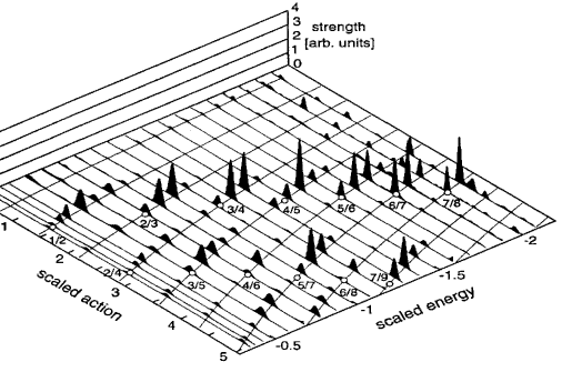
Figure 3: Experimental recurrence spectra of lithium in an electric field in overlay form. The curves mark the scaled action of the parallel orbit and its repetitions as a function of scaled energy. The open circles mark the bifurcation points of closed orbits, whose shapes are shown along the bottom. (From Ref. [52].)

Scaled energy spectroscopy has become a well established method to investigate the dynamics of hydrogenic and nonhydrogenic atoms in external fields. Recurrence spectra of helium in a magnetic field are presented in Ref. [48, 49]. Recurrence peaks of the helium atom which cannot be identified by hydrogenic closed orbits have been explained by scattering of the highly excited electron at the ionic core [49, 75, 76]. Rubidium has been studied in crossed electric and magnetic fields in Ref. [50] and unidentified recurrence peaks have been interpreted in terms of classical core scattering [77]. The Stark effect on lithium has been investigated by the MIT group [51, 52, 53]. For atoms in an electric field $F$ the scaling parameter is $w\equiv F^{-1/4}$, and $EF^{-1/2}$ is the scaled energy. Experimental recurrence spectra of lithium in an electric field and the corresponding closed orbits are presented in Fig. 3. Strong recurrence peaks occur close to the bifurcations of the parallel orbit and its repetitions marked by open circles in Fig. 3. The new orbits created in bifurcations have almost the same action as the corresponding return of the parallel orbit, and, similar as in Fig. 1 for the hydrogen atom in a magnetic field, the small splittings of recurrence peaks are not resolved in the experimental recurrence spectra.

It is important to note that the finite resolution of the experimental recurrence spectra in Figs. 1 and 3 is not caused by the finite bandwidth of the exciting laser but results as discussed above from the finite length of the Fourier transformed scaled spectra and the uncertainty principle of the Fourier transform. This can be illustrated by analyzing a numerically computed spectrum instead of an experimentally measured spectrum. We study the hydrogen atom in a magnetic field at constant scaled energy $\tilde{E}=-0.1$. At this energy the classical dynamics is completely chaotic and all periodic orbits are unstable. We calculated 9715 states in the region $w<140$ by numerical diagonalization of the Hamiltonian matrix in a complete basis set. For details of the quantum calculations see, e.g., Ref. [96]. In Fig. 4 the quantum density of states is analyzed by the conventional Fourier transform. To get rid of unphysical side-peaks the spectrum was multiplied with a Gaussian function $h(w)$ with width $\sigma$ chosen in accordance with the total length of the quantum spectrum. Fig. 4 clearly exhibits recurrence peaks which can be related to classical periodic orbits. However, the widths of the peaks are approximately $\Delta s/2\pi=0.03$, and it is impossible to determine the periods of the classical orbits to higher accuracy than about $0.01$ from the Fourier analysis of the quantum spectrum. Recurrence peaks of orbits with similar periods overlap, as can be clearly seen around $s/2\pi=2.1$, and at least guessed, e.g., at $s/2\pi=1.1$, or $s/2\pi=2.6$. A precise determination of the amplitudes is impossible especially for the overlapping peaks. Furthermore, the Fourier transform does not allow to distinguish between real and ghost orbits. In the following we will demonstrate that the quality of recurrence spectra can be significantly improved by application of state of the art methods for high resolution spectral analysis.

2.2 Circumventing the uncertainty principle

Instead of using the standard Fourier analysis, to extract the amplitudes and actions we propose to apply methods for high resolution spectral analysis. The fundamental difference between the Fourier transform and high resolution methods is the following. Assume a complex signal $C(t)$ given on an equidistant grid of points $t_{n}=t_{0}+n\Delta t$ as a superposition of exponential functions, i.e.

$$C(t_{n})\equiv c_{n}=\sum_{k}d_{k}e^{-it_{n}\omega_{k}}\;,\quad n=1,2,\dots,N\;.$$ (2.14)

In the Discrete Fourier Transform (DFT) $N$ real frequencies

$$\omega_{k}={2\pi k\over N\Delta t}\;,\quad k=1,2,\dots,N$$ (2.15)

are fixed and evenly spaced. The $N$ complex amplitudes $d_{k}$ of the Fourier transform are determined by solving a linear set of equations, yielding

$$d_{k}={1\over{N}}\sum_{n=1}^{N}c_{n}e^{it_{n}\omega_{k}}\;,\quad k=1,2,\dots,N\;.$$ (2.16)

The sums in Eq. 2.16 can be calculated numerically very efficiently, e.g., by the Fast Fourier Transform algorithm (FFT). The resolution $\Delta\omega$ of the Fourier transform is controlled by the total length $N\Delta t$ of the signal,

$$\Delta\omega={2\pi\over N\Delta t}\;,$$ (2.17)

which is the spacing between the grid points in the frequency domain. Only those spectral features that are separated from each other by more than $\Delta w$ can be resolved. This is referred to as the “uncertainty principle” of the Fourier transform. By contrast, both the amplitudes $d_{k}$ and the frequencies $\omega_{k}$ in Eq. 2.14 are free parameters when methods for high resolution spectral analysis are applied. Because the frequencies $\omega_{k}$ are free adjusting parameters they are allowed to appear very close to each other and therefore the resolution is practically infinite. Using the data points of the signal $C(t)$ at $t=t_{n}$ the set of in general complex parameters $\{d_{k},\omega_{k}\}$ are given as the solution of a nonlinear set of equations. Unfortunately, the nonlinear set of equations does not have a solution in closed form similar to Eq. 2.16 for the discrete Fourier transform. In fact, the numerical calculation of the parameters $\{d_{k},\omega_{k}\}$ from the nonlinear set of equations is the central and nontrivial problem of all methods for high resolution spectral analysis.

The numerical harmonic inversion of a given signal like Eq. 2.14 is a fundamental problem in physics, electrical engineering and many other diverse fields. The problem has already been addressed (in a slightly different form) in the 18th century by Baron de Prony, who converted the nonlinear set of equations (2.14) to a linear algebra problem. There are several approaches related to the Prony method used for a high resolution spectral analysis of short time signals, such as the modern versions of the Prony method, MUSIC (MUltiple SIgnal Classification) and ESPRIT (Estimation of Signal Parameters via Rotational Invariance Technique) [67, 97, 98]. As opposed to the Fourier transform these methods are not related to a linear (unitary) transformation of the signal and are highly nonlinear by their nature. However, the common feature present in most versions of these methods is converting the nonlinear fitting problem to a linear algebraic one. Note also that while ESPRIT uses exclusively linear algebra, the Prony method or MUSIC require some additional search in the frequency domain which makes them less efficient. To our best knowledge none of these nonlinear methods is able to handle a signal (2.14) that contains “too many” frequencies as they lead to unfeasibly large and typically ill-conditioned linear algebra problems [70]. This is especially the case for the analysis of quantum spectra because such spectra cannot be treated as “short signals” and contain a high number of frequencies given by (see below) the number of periodic orbits of the underlying classical system. Decisive progress in the numerical techniques for harmonic inversion has recently been achieved by Wall and Neuhauser [68]. Their method is conceptually based on the original filter-diagonalization method of Neuhauser [99] designed to obtain the eigenspectrum of a Hamiltonian operator in any selected small energy range. The main idea is to associate the signal $C(t)$ (Eq. 2.14) with an autocorrelation function of a suitable dynamical system,

$$C(t)=\left(\Phi_{0},e^{-i\hat{\Omega}t}\Phi_{0}\right)\;,$$ (2.18)

where the brackets define a complex symmetric inner product (i.e., no complex conjugation). Eq. 2.18 establishes an equivalence between the problem of extracting information from the signal $C(t)$ with the one of diagonalizing the evolution operator $\exp(-i\hat{\Omega})$ of the underlying dynamical system. The frequencies $\omega_{k}$ of the signal $C(t)$ are the eigenvalues of the operator $\hat{\Omega}$, i.e.

$$\hat{\Omega}|\Phi_{k})=\omega_{k}|\Phi_{k})\;,$$ (2.19)

and the amplitudes $d_{k}$ are formally given as

$$d_{k}=\left(\Phi_{0},\Phi_{k}\right)^{2}\;.$$ (2.20)

After introducing an appropriate basis set, the operator $\exp(-i\hat{\Omega})$ can be diagonalized using the method of filter-diagonalization [68, 69, 70]. Operationally this is done by solving a small generalized eigenvalue problem whose eigenvalues yield the frequencies in a chosen window. Typically, the numerical handling of matrices with approximate dimension $100\times 100$ is sufficient even when the number of frequencies in the signal $C(s)$ is about $10000$ or more. The knowledge of the operator $\hat{\Omega}$ itself is not required as for a properly chosen basis the matrix elements of $\hat{\Omega}$ can be expressed only in terms of the signal $C(t)$. The advantage of the filter-diagonalization technique is its numerical stability with respect to both the length and complexity (the number and density of the contributing frequencies) of the signal. Details of the method of harmonic inversion by filter-diagonalization are given in Ref. [70] and in Appendix A.1.

We now want to apply harmonic inversion as a tool for the high precision analysis of quantum spectra. In quantum calculations the bound state spectrum is given as a sum of $\delta$-functions,

$$\varrho^{\rm qm}(w)=\sum_{k}\delta(w-w_{k})\;.$$ (2.21)

Instead of using the Fourier transform (Eq. 2.7) we want to adjust $\varrho^{\rm qm}(w)$ to the functional form of Gutzwiller’s semiclassical trace formula (2.3), which can be written as

$$\varrho^{\rm sc}(w)=\varrho_{0}(w)+{1\over 2\pi}\sum_{\rm po}\sum_{r=1}^{\infty}\left\{A_{\rm po,r}e^{irs_{\rm po}w}+A_{\rm po,r}^{\ast}e^{-irs_{\rm po}^{\ast}w}\right\}\;.$$ (2.22)

The fluctuating part of the semiclassical density of states (2.22) has exactly the functional form of the signal $C(t)$ in Eq. 2.14 with $t$ replaced by the scaling parameter $w$. The amplitudes and frequencies $\{d_{k},\omega_{k}\}$ in Eq. 2.14 are the amplitudes and scaled actions $\{A_{\rm po,r}/2\pi,-rs_{\rm po}\}$ of the periodic orbit contributions and their conjugate pairs $\{A_{\rm po,r}^{\ast}/2\pi,rs_{\rm po}^{\ast}\}$. In order to obtain $\varrho^{\rm qm}(w)$ on an evenly spaced grid the spectrum is regularized by convoluting it with a narrow Gaussian function having the width $\sigma\ll 1/s_{\rm max}$, where $s_{\rm max}$ is the scaled action of the longest orbit of interest. The regularized density of states reads

$$\varrho_{\sigma}^{\rm qm}(w)=\sum_{k}\delta_{\sigma}(w-w_{k})={1\over\sqrt{2\pi}\sigma}\sum_{k}e^{-{(w-w_{k})^{2}/2\sigma^{2}}}\;,$$ (2.23)

and is the starting point for the harmonic inversion procedure. The step width for the discretization of $\varrho_{\sigma}^{\rm qm}(w)$ is typically chosen as $\Delta w\approx\sigma/3$. The convolution of $\varrho^{\rm qm}(w)$ with a Gaussian function does not effect the frequencies, i.e., the values obtained for the scaled actions $s_{\rm po}$ of the periodic orbits, but just results in a small damping of the amplitudes

$$A_{\rm po,r}\longrightarrow A_{\rm po,r}^{(\sigma)}=A_{\rm po,r}e^{-s_{\rm po}^{2}\sigma^{2}/2}\;.$$ (2.24)

For open systems the density of states is given by

$$\varrho^{\rm qm}(w)=-{1\over\pi}\,{\rm Im}\,\sum_{k}{1\over w-w_{k}}\;,$$ (2.25)

with complex resonances $w_{k}$. If the minimum of the resonance widths $\Gamma_{k}=-2\,{\rm Im}\,w_{k}$ is larger than the step width $\Delta w$, there is no need to convolute $\varrho^{\rm qm}(w)$ with a Gaussian function and the density of states can directly be analyzed by harmonic inversion in the same way as for bound systems.

2.3 Precision check of the periodic orbit theory

As a first application of harmonic inversion for the high resolution analysis of quantum spectra we investigate the hydrogen atom in a magnetic field given by the Hamiltonian (2.11) and compare the results of the harmonic inversion method to the conventional Fourier transform presented in Fig. 4. We analyze the density of states (2.23) with $\sigma=0.0015$ at constant scaled energy $\tilde{E}=-0.1$. From the discussion of the harmonic inversion technique and especially Eq. 2.19 it follows that the frequencies in $\varrho_{\sigma}^{\rm qm}(w)$, i.e., the actions of periodic orbits, are not obtained from a continuous frequency spectrum (or a spectrum defined on an equidistant grid of frequencies) but are given as discrete and in general complex eigenvalues. Actions with imaginary part significantly below zero indicate “ghost” orbit contributions to the quantum spectrum. The actions $s_{\rm po}^{\rm qm}/2\pi$ and absolute values of the amplitudes $|A^{\rm qm}|$ are given in the first three columns of Table 1. The last two columns present the classical actions $s_{\rm po}^{\rm cl}/2\pi$ of the periodic orbits and the absolute values of the semiclassical amplitudes

$$|A^{\rm cl}|={s_{\rm po}^{\rm prim}/2\pi\over\sqrt{|{\rm det}(M_{\rm po}-I)|}}\;,$$ (2.26)

with $s_{\rm po}^{\rm prim}$ the action of the primitive periodic orbit, i.e., the first recurrence of the orbit. A graphical comparison between the Fourier transform, the high resolution quantum recurrence spectrum, and the semiclassical recurrence spectrum is presented in Fig. 5. The crosses in Fig. 5b are the (complex) actions obtained by the harmonic inversion of the quantum mechanical density of states, and the squares are the actions of the (real) classical periodic orbits. The crosses and squares are in excellent agreement with a few exceptions, e.g., around $s/2\pi\approx 2.2$ and $s/2\pi\approx 2.8$ which will be discussed later. The amplitudes of the periodic orbit contributions are illustrated in Fig. 5a. The solid sticks are the amplitudes obtained by harmonic inversion of the quantum spectrum and the dashed sticks (hardly visible under solid sticks) present the corresponding semiclassical results. For comparison, the conventional Fourier transform recurrence spectrum is drawn as a solid line. To visualize more clearly the improvement of the high resolution recurrence spectrum compared to the conventional Fourier transform a small part of the recurrence spectrum (Fig. 5a) around $s/2\pi=2.6$ is enlarged in Fig. 6. The smooth line is the absolute value of the conventional Fourier transform. Its shape suggests the existence of at least three periodic orbits but obviously the recurrence spectrum is not completely resolved. The results of the high resolution spectral analysis are presented as sticks and crosses at the positions defined by the scaled actions $s_{\rm po}^{\rm qm}$ with peak heights $|A^{\rm qm}|$. Note that the positions of the peaks are considerably shifted with respect to the maxima of the conventional Fourier transform. To compare the quantum recurrence spectrum with Gutzwiller’s periodic orbit theory the semiclassical results are presented as dashed sticks and squares in Fig. 6. For illustration the shapes of periodic orbits are also shown (in semiparabolic coordinates $\mu=\sqrt{r+z}$, $\nu=\sqrt{r-z}$). For these three orbits the agreement between the semiclassical and the high resolution quantum recurrence spectrum is nearly perfect, deviations are within the stick widths. The relative deviations between the quantum mechanical and classical actions and amplitudes are given in Table 2.

The excellent agreement between the classical periodic orbit data and the quantum mechanical results obtained by harmonic inversion of the density of states may appear to be in contradiction to the fact that Gutzwiller’s trace formula is an approximation, i.e., only the leading term of the semiclassical $\hbar$ expansion of the periodic orbit sum. The small deviations given in Table 2 are certainly due to numerical limitations and do not indicate effects of higher order $\hbar$ corrections. The reason is that the higher order $\hbar$ contributions of the periodic orbits do not have the functional form of Eq. 2.22 as a linear superposition of exponential functions of the scaling parameter $w$. As the harmonic inversion procedure adjusts the quantum mechanical density of states $\varrho^{\rm qm}(w)$ to the ansatz (2.22) with free parameters $s_{\rm po}$ and $A_{\rm po}$, the exact parameters $s_{\rm po}$ and $A_{\rm po}$ of the classical periodic orbits should provide the optimal adjustment to the quantum spectrum within the lowest order $\hbar$ approximation. However, the harmonic inversion technique can also be used to reveal the higher order $\hbar$ contributions of the periodic orbits in the quantum spectra, as will be demonstrated in Section 2.6.

The quantum mechanical high resolution recurrence spectrum is not in good agreement with the classical calculations around $s/2\pi\approx 2.2$ (see crosses and squares in Fig. 5b). This period is close to the scaled action $s_{\rm po}/2\pi=(-2\tilde{E})^{-1/2}=2.2361$ of the parallel orbit, which undergoes an infinite series of bifurcations with increasing energy [100]. If orbits are too close to bifurcations they can no longer be treated as isolated periodic orbits, which in turn is the basic assumption for Gutzwiller’s semiclassical trace formula (2.3). The disagreement between the crosses and squares in Fig. 5 around $s/2\pi\approx 2.2$ thus indicates the breakdown of the semiclassical ansatz (2.3) for non-isolated orbits. The structures around $s/2\pi\approx 2.8$ can also not be explained by real classical periodic orbits. They are related to uniform semiclassical approximations and complex ghost orbits as will be discussed in the next section.

2.4 Ghost orbits and uniform semiclassical approximations

Gutzwiller’s periodic orbit theory (2.3) is valid for isolated periodic orbits where the determinant $\det(M_{\rm po}^{r}-I)$, i.e., the denominator in Eq. 2.5 is nonzero. However, the periodic orbit amplitudes $A_{{\rm po},r}$ diverge close to the bifurcation points of orbits where $M_{\rm po}^{r}-I$ has a vanishing determinant. To remove the unphysical singularity from the semiclassical expressions all periodic orbits which participate at the bifurcation must be considered simultaneously in a uniform semiclassical approximation [40, 41]. The uniform solutions can be constructed with the help of catastrophe theory [38, 39], and have been studied, e.g., for the kicked top [36, 42, 43, 101] and the hydrogen atom in a magnetic field [37, 44]. In the vicinity of bifurcations “ghost” orbits, i.e., periodic orbits in the complex continuation of phase space can be very important. In general the ghost orbits have real or complex actions, $s_{\rm po}$. As can be shown from the asymptotic expansions of the uniform semiclassical approximations [37, 44] those ghosts with positive imaginary part of the action, ${\rm Im}\,s_{\rm po}>0$, are of physical relevance. They contribute as

$$A_{\rm po}\,e^{i\,{\rm Re}\,s_{\rm po}w}\,e^{-\,{\rm Im}\,s_{\rm po}w}$$

to Gutzwiller’s periodic orbit sum (2.3), i.e., the modulations of the ghost orbits are exponentially damped with increasing scaling parameter $w$.

Here we will only present a brief derivation of uniform semiclassical approximations. For details we refer the reader to the literature [36, 37, 42, 43, 44, 101]. Our main interest is to demonstrate how bifurcations and ghost orbits can directly be uncovered in quantum spectra with the help of the harmonic inversion technique and the high resolution recurrence spectra. Note that a detailed investigation of these phenomena is in general impossible with the Fourier transform because the orbits participating at the bifurcation have nearly the same period and thus cannot be resolved in the conventional recurrence spectra. We will discuss two different types of bifurcations by way of example of the hydrogen atom in a magnetic field: The hyperbolic umbilic and the butterfly catastrophe.

In the following section we will adopt the symbolic code of Ref. [102] for the nomenclature of periodic orbits. Introducing scaled semiparabolic coordinates $\mu=\gamma^{1/3}\sqrt{r+z}$ and $\nu=\gamma^{1/3}\sqrt{r-z}$ the scaled Hamiltonian of the hydrogen atom in a magnetic field reads

$$h={1\over 2}(p_{\mu}^{2}+p_{\nu}^{2})-\tilde{E}(\mu^{2}+\nu^{2})+{1\over 8}(\mu^{4}\nu^{2}+\mu^{2}\nu^{4})=2\;.$$ (2.27)

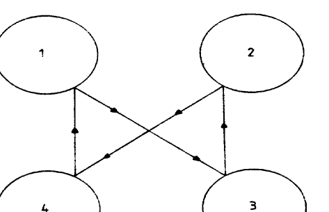
Figure 7: Schematic view of the four-disk scattering problem. (From Ref. [102].)

As pointed out in [102] the effective potential $V(\mu,\nu)=-\tilde{E}(\mu^{2}+\nu^{2})+(\mu^{4}\nu^{2}+\mu^{2}\nu^{4})/8$ is bounded for $\tilde{E}>0$ by four hyperbolas. When the smooth potential is replaced with hard walls periodic orbits can be assigned with the same ternary symbolic code as orbits of the four-disk scattering problem (see Fig. 7). In a first step a ternary alphabet {0AC} is introduced. The symbol 0 labels scattering to the opposite disk, and the symbols C and A label scattering to the neighboring disk in clockwise or anticlockwise direction, respectively. The orbit in Fig. 7 is coded 0C0A. The ternary code can be made more efficient with respect to the exchange symmetry of the C and A symbol if it is redefined in the following way. The Cs and As are replaced with the sympol +, if consecutive letters ignoring the 0s are equal and they are replaced with the symbol -, if consecutive letters differ. With this redefinition the orbit shown in Fig. 7 is coded 0-0-, or because of its periodicity even simpler 0-. For the hydrogen atom in a magnetic field there is a one to one correspondence between the periodic orbits and the ternary symbolic code at energies $\tilde{E}>\tilde{E}_{c}=+0.3287$ [19, 21]. Below the critical energy orbits undergo bifurcations and the code is not unique. However, nearly all unstable periodic orbits can be uniquely assigned with this code even at negative energies.

2.4.1 The hyperbolic umbilic catastrophe

As a first example we investigate the structure at $s_{\rm po}/2\pi=2.767$ in the recurrence spectrum of the hydrogen atom in a magnetic field at constant scaled energy $\tilde{E}=E\gamma^{-2/3}=-0.1$ (see Fig. 5 and Table 1). At this energy no periodic orbit with an action close to $s_{\rm po}/2\pi=2.767$ does exist. However, the strong recurrence peak in Fig. 5a indicates a near bifurcation. This bifurcation and the corresponding semiclassical approximation have been studied in detail in Refs. [44, 80]. Four periodic orbits are created through two nearby bifurcations around the scaled energy $\tilde{E}\approx-0.096$ where we search for both real and complex “ghost” orbits. For the nomenclature of the real orbits we adopt the symbolic code of Ref. [102] as explained above. At scaled energy $\tilde{E}_{b}^{(1)}=-0.09689$, the two orbits 00+- and +++--- are born in a tangent bifurcation. At energies $\tilde{E}<\tilde{E}_{b}^{(1)}$, a prebifurcation ghost orbit and its complex conjugate exist in the complex continuation of the phase space. Orbit 00+- is born unstable, and turns stable at the slightly higher energy $\tilde{E}_{b}^{(2)}=-0.09451$. This is the bifurcation point of two additional orbits, 0-+-- and its time reversal 0---+, which also have ghost orbits as predecessors. The graphs of the real orbits at energy $E=0$ are shown as insets in Fig. 8, and the classical periodic orbit parameters are presented as solid lines in Figs. 8 and 9. Fig. 8 shows the difference in scaled action between the orbits. The action of orbit 0-+-- (or its time reversal 0---+), which is real also for its prebifurcation ghost orbits, has been taken as the reference action. The uniform semiclassical approximation for the four orbits involved in the bifurcation can be expressed in terms of the diffraction integral of a hyperbolic umbilic catastrophe

$$\Psi(x,y)=\int_{-\infty}^{+\infty}dp\int_{-\infty}^{+\infty}dqe^{i\Phi(p,q;x,y)}$$ (2.28)

with

$$\Phi(p,q;x,y)=p^{3}+q^{3}+y(p+q)^{2}+x(p+q)\;.$$ (2.29)

For our convenience the function $\Phi(p,q;x,y)$ slightly differs from the standard polynomial of the hyperbolic umbilic catastrophe given in Ref. [39] but the diffraction integral (2.28) can be easily transformed to the standard representation. The four stationary points of the integral (2.28) are readily obtained from the condition $\nabla\Phi=0$ as

$$p_{0}=-q_{0}=\pm\sqrt{-x/3}\Rightarrow\Phi(p_{0},q_{0};x,y)=0$$ (2.30)

and

$$p_{0}=q_{0} = -{2\over 3}y\pm\sqrt{{4\over 9}y^{2}-{x\over 3}}\Rightarrow$$

$$\Phi(p_{0},q_{0};x,y) = {4\over 3}y\left({8\over 9}y^{2}-x\right)\mp 4\left({4\over 9}y^{2}-{x\over 3}\right)^{3/2}\;.$$ (2.31)

The function $\Phi(p_{0},q_{0};x,y)$ must now be adapted to the classical action of the four periodic orbits, i.e., $\Delta S=w\Delta s\approx\Phi(p_{0},q_{0};x,y)$, which is well fulfilled for

$$x=aw^{2/3}\left(\tilde{E}-\tilde{E}_{b}^{(2)}\right)\;;\quad y=bw^{1/3}\;,$$ (2.32)

and constants $a=-5.415$, $b=0.09665$, as can be seen from the dashed lines in Fig. 8. Note that the agreement holds for both the real and complex ghost orbits.

The next step to obtain the uniform solution is to calculate the diffraction integral (2.28) within the stationary phase approximation. For $\tilde{E}>\tilde{E}_{b}^{(2)}$ there are four real stationary points $(p_{0},q_{0})$ (see Eqs. 2.30 and 2.31), and after expanding $\Phi(p,q;x,y)$ around the stationary points up to second order in $p$ and $q$, the diffraction integral becomes the sum of Fresnel integrals, viz.

$$\Psi(x,y)\stackrel{{\scriptstyle x\ll 0}}{{\sim}}{2\pi\over\sqrt{-3x}}+\sum_{+,-}{\pi e^{i\left[{4\over 3}y\left({8\over 9}y^{2}-x\right)\mp 4\left({4\over 9}y^{2}-{x\over 3}\right)^{3/2}\pm{\pi\over 2}\right]}\over\sqrt{(4y^{2}-3x)\mp 2y\sqrt{4y^{2}-3x}}}\,.$$ (2.33)

The terms of Eq. 2.33 can now be compared to the standard periodic orbit contributions (2.26) of Gutzwiller’s trace formula. In our example the first term is related to the orbit 0-+-- (with a multiplicity factor of 2 for its time reversal 0---+), and the other two terms are related to the orbits 00+- and +++--- for the upper and lower sign, respectively. The phase shift in the numerators describe the differences of the action $\Delta S$ and of the Maslov index $\Delta\mu=\mp 1$ relative to the reference orbit 0-+--. The denominators are, up to a factor $cw^{1/3}$, with $c=0.1034$, the square root of $|\det(M-I)|$, with $M$ the stability matrix. Fig. 9 presents the comparison for the determinants obtained from classical periodic orbit calculations (solid lines) and from Eqs. 2.32 and 2.33 (dashed lines). The agreement is very good for both the real and complex ghost orbits, similar to the agreement found for $\Delta s$ in Fig. 8. The constant $c$ introduced above determines the normalization of the uniform semiclassical approximation for the hyperbolic umbilic bifurcation which is finally obtained as [44, 80]

$${\cal A}_{\rm uniform}(\tilde{E},w)=(c/\pi)s_{0}w^{1/3}\,\Psi\left(aw^{2/3}(\tilde{E}-\tilde{E}_{b}^{(2)}),bw^{1/3}\right)e^{i[s_{0}w-{\pi\over 2}\mu_{0}]}\;,$$

(2.34)

with $s_{0}$ and $\mu_{0}$ denoting the orbital action and Maslov index of the reference orbit 0-+--, and the constants $a$, $b$, and $c$ as given above.

The comparison between the amplitudes (2.26) of the conventional semiclassical trace formula for isolated periodic orbits and the uniform approximation (2.34) for the hyperbolic umbilic catastrophe is presented in Fig. 10 at the magnetic field strengths $\gamma=10^{-7}$, $\gamma=10^{-8}$, and $\gamma=10^{-9}$. For graphical purposes we suppress the highly oscillatory part resulting from the function $\exp[i(S_{0}/\hbar-{\pi\over 2}\mu_{0})]$ by plotting the absolute value of ${\cal A}(\tilde{E},w)$ instead of the real part. The dashed line in Fig. 10 is the superposition of the isolated periodic orbit contributions from the four orbits involved in the bifurcations. The modulations of the amplitude are caused by the constructive and destructive interference of the real orbits at energies $\tilde{E}>\tilde{E}_{b}^{(2)}$ and are most pronounced at low magnetic field strength (see Fig. 10c). The amplitude diverges at the two bifurcation points. For the calculation of the uniform approximation (2.34) we numerically evaluated the catastrophe diffraction integral (2.28) using a more simple and direct technique as described in [103]. Details of our method which is based on Taylor series expansions are given in Appendix C.1. The solid line in Fig. 10 is the uniform approximation (2.34). It does not diverge at the bifurcation points but decreases exponentially at energies $\tilde{E}<\tilde{E}_{b}^{(1)}$. At these energies no real orbits exist and the amplitude in the standard formulation would be zero when only real orbits are considered. However, the exponential tail of the uniform approximation (2.34) is well reproduced by a ghost orbit [37, 36] with positive imaginary part of the complex action. As can be shown, the asymptotic expansion of the diffraction integral (2.28) has, for $x\gg 0$, exactly the form of Eq. 2.26 but with complex action $s$ and determinant $\det(M-I)$. The ghost orbit contribution is shown as dash-dotted line in Fig. 10.

To verify the hyperbolic umbilic catastrophe in the quantum spectrum we analyze all three, the exact quantum spectrum, the uniform semiclassical approximation (2.34), and Gutzwiller’s periodic orbit formula for isolated periodic orbits by means of the harmonic inversion technique at scaled energy $\tilde{E}=-0.1$, which is slightly below the two bifurcation points. The part of the complex action plane which is of interest for the hyperbolic umbilic catastrophe is presented in Fig. 11. The two solid peaks mark the positions $s_{k}/2\pi$ and the absolute values of amplitudes $|A_{k}|$ obtained from the quantum spectrum. As mentioned above, at this energy only one classical ghost orbit is of physical relevance and marked as dash-dotted peak in Fig. 11. The position of that peak is in good agreement with the quantum result but the amplitude is enhanced. This enhancement is expected for isolated periodic orbit contributions near bifurcations which become singular exactly at the bifurcation points. The harmonic inversion analysis of the uniform approximation (2.34) at constant scaled energy $\tilde{E}=-0.1$ in the same range $0<w<140$ is presented as dashed peaks in Fig. 11. The two peaks agree well with the quantum results for both the complex actions and amplitudes. The enhancement of the ghost orbit peak and the additional non-classical peak observed in the quantum spectrum are therefore clearly identified as artifacts of the bifurcation, i.e., the hyperbolic umbilic catastrophe.

2.4.2 The butterfly catastrophe: Uncovering the “hidden” ghost orbits

We now investigate the butterfly catastrophe, which is of importance, e.g., in photoabsorption spectra of the hydrogen atom in a magnetic field. In contrast to the density of states the photoabsorption spectra for dipole transitions from a low-lying initial state to highly excited final states can be measured experimentally [45, 46, 47]. The semiclassical photoabsorption cross-section is obtained by closed orbit theory [90, 91, 92, 93] as the superposition of a smooth background and sinusoidal modulations induced by closed orbits starting at and returning back to the nucleus. Although the derivation of the semiclassical oscillator strength for dipole transitions (closed orbit theory) differs from the derivation of the semiclassical density of states (periodic orbit theory) the final results have a very similar structure and therefore spectra can be analyzed in the same way by conventional Fourier transform or the high resolution harmonic inversion technique. In closed orbit theory the semiclassical oscillator strength is given by

$$f=f^{0}+f^{\rm osc}$$ (2.35)

with $f^{0}$ the oscillator strength of the field free hydrogen atom at energy $E=0$ and

$$f^{\rm osc} = 2(E_{f}-E_{i})w^{-1/2}\,{\rm Im}\,\sum_{{\rm cl.o.}~{}k}{2(2\pi)^{3/2}\over\sqrt{|\tilde{m}_{12}^{(k)}|}}\sqrt{\sin\vartheta_{i,k}\vartheta_{f,k}}$$ (2.36)

$$\times {\cal Y}_{m}(\vartheta_{i,k}){\cal Y}_{m}(\vartheta_{f,k})\exp\left\{i\left(s_{k}w+{1\over 2}m\tilde{T}_{k}-{\pi\over 2}\mu_{k}^{0}+{\pi\over 4}\right)\right\}$$

the fluctuating part of the oscillator strength. In (2.36) $E_{f}$ and $E_{i}$ are the energies of the final and initial state, $m$ is the magnetic quantum number, $s_{k}$, $\tilde{T}_{k}=\gamma T_{k}$, and $\mu_{k}^{0}$ are the scaled action, scaled time, and the Maslov index of closed orbit $k$, $\vartheta_{i}$ and $\vartheta_{f}$ are the starting and returning angle of the orbit with respect to the magnetic field axis, and $\tilde{m}_{12}$ is an element of the scaled monodromy matrix. The angular functions ${\cal Y}_{m}(\vartheta)$ depend on the initial state and polarization of light (see Appendix B). For more details see Refs. [47, 91, 93]. The fluctuating terms (2.36) of the photoabsorption cross section are sinusoidal functions of the scaling parameter $w=\gamma^{-1/3}$ despite a factor of $w^{-1/2}$. To obtain the same functional form as Eq. 2.22 for the density of states, which is required for harmonic inversion, we multiply the oscillator strength $f$ by $w^{1/2}$ for both the semiclassical and quantum mechanical photoabsorption spectra.

In analogy to Gutzwiller’s trace formula Eq. 2.36 for photoabsorption spectra is valid only for isolated orbits and diverges at bifurcations of orbits, where $\tilde{m}_{12}$ is zero. Near bifurcations the closed orbit contributions in (2.36) must be replaced with uniform semiclassical approximations, which have been studied in detail for the fold, cusp, and butterfly catastrophe in Refs. [37, 81]. Here we restrict the discussion to the butterfly catastrophe, which is especially interesting because of the existence of a “hidden” ghost orbit, which can be uncovered in the photoabsorption spectrum of the hydrogen atom in a magnetic field with the help of the harmonic inversion technique. As an example we investigate real and ghost orbits related to the period doubling of the perpendicular orbit $R_{1}$. (For the closed orbits we adopt the nomenclature of Refs. [45, 46], see also Fig. 2.) This closed orbit bifurcation is more complicated because various orbits with similar periods undergo two different elementary types of bifurcations at nearly the same energy. The structure of bifurcations and the appearance of ghost orbits can clearly be seen in the energy dependence of the starting angles $\vartheta_{i}$ in Fig. 12a. Two orbits $R_{2}^{1}$ and $R_{2}^{1b}$ are born in a saddle node bifurcation at $\tilde{E}_{b}^{(1)}=-0.31735345$, $\vartheta_{i}=1.3465$. Below the bifurcation energy we find an associated ghost orbit and its complex conjugate. Orbit $R_{2}^{1b}$ is real only in a very short energy interval ($\Delta\tilde{E}\approx 0.001$), and is then involved in the next bifurcation at $\tilde{E}_{b}^{(2)}=-0.31618537$, $\vartheta_{i}=\pi/2$. This is the period doubling bifurcation of the perpendicular orbit $R_{1}$, which exists at all energies ($\vartheta_{i}=\pi/2$ in Fig. 12a). The real orbit $R_{2}^{1b}$ separates from $R_{1}$ at energies below the bifurcation point, i.e. a real orbit vanishes with increasing energy. Consequently, associated ghost orbits are expected at energies above the bifurcation, i.e. $\tilde{E}>\tilde{E}_{b}^{(2)}$, and indeed such “postbifurcation” ghosts have been found. Its complex starting angles are also shown in Fig. 12a. The energy dependence of scaled actions, or, more precisely, the difference $\Delta s$ with respect to the action of the period doubled perpendicular orbit $R_{2}$, is presented in Fig. 12b (solid lines), and the graph for the monodromy matrix element $\tilde{m}_{12}$ is given in Fig. 12c. It can be seen that the actions and the monodromy matrix elements of the ghost orbits related to the saddle node bifurcation of $R_{2}^{1}$ become complex at $\tilde{E}<\tilde{E}_{b}^{(1)}$, while these parameters remain real for the postbifurcation ghosts at $\tilde{E}>\tilde{E}_{b}^{(2)}$. The two bifurcations are so closely adjacent that formulae for the saddle node bifurcation and the period doubling are no reasonable approximation to $\Delta s(\tilde{E})$ and $\tilde{m}_{12}(\tilde{E})$ in the neighborhood of the bifurcations. However, both functions can be fitted well by the more complicated formulae [37]

$$\Delta s=k\left(\tilde{\sigma}\left({\tilde{E}}-{\tilde{E}}_{b}^{(2)}\right)+{2\over 3}\left\{1\pm\left[\tilde{\sigma}\left({\tilde{E}}-{\tilde{E}}_{b}^{(2)}\right)+1\right]^{3/2}\right\}\right)$$ (2.37)

and

$$\tilde{m}_{12} = -\tilde{M}\left({\tilde{E}}-{\tilde{E}}_{b}^{(2)}\right)~{}~{}~{}~{}({\rm orbit}~{}R_{2})$$

$$\tilde{m}_{12} = 4\tilde{M}\left({\tilde{E}}-{\tilde{E}}_{b}^{(2)}\right)+{4\tilde{M}\over\tilde{\sigma}}\left[1\pm\sqrt{\tilde{\sigma}\left({\tilde{E}}-{\tilde{E}}_{b}^{(2)}\right)+1}\right]$$

$$(R_{2}^{1},R_{2}^{1b},~{}{\rm and~{}ghosts})$$

with $k=3.768\cdot 10^{-4}$, $\tilde{\sigma}=763.6$, and $\tilde{M}=13.52$ (see dashed lines in Figs. 12b and 12c). Note that Eqs. (2.37) and (2.4.2) describe the complete scenario for the real and the ghost orbits including both the saddle node and period doubling bifurcations. We also mention that orbits with angles $\vartheta_{i}\neq\vartheta_{f}$ have to be counted twice because they correspond to different orbits when traversed in either direction, and therefore a total number of five closed orbits, including ghosts, is considered here in the bifurcation scenario around the period doubling of the perpendicular orbit.

The bunch of trajectories forming the butterfly is given by the Hamilton-Jacobi equations (with $p_{\xi}=\partial S/\partial\xi$ and $p_{\eta}=\partial S/\partial\eta$)

$$3dp_{\eta}^{5}+2cp_{\xi}^{2}p_{\eta}^{3}+p_{\xi}^{4}\left[(\xi-\xi_{0})p_{\eta}-\eta p_{\xi}\right] = 0$$

$$p_{\xi}^{2}+p_{\eta}^{2} = 4\;,$$ (2.39)

where $\xi$ and $\eta$ are rotated semiparabolic coordinates

$$\xi = \mu\cos{\vartheta_{f}\over 2}+\nu\sin{\vartheta_{f}\over 2}=\sqrt{2r}\cos{\vartheta-\vartheta_{f}\over 2}$$ (2.40)

$$\eta = \nu\cos{\vartheta_{f}\over 2}-\mu\sin{\vartheta_{f}\over 2}=\sqrt{2r}\sin{\vartheta-\vartheta_{f}\over 2}\;,$$ (2.41)

so that the $\xi$ and $\eta$ axes are now parallel and perpendicular to the returning orbit. The parameters $c$, $d$, and $\xi_{0}$ in Eq. 2.39 will be specified later. With $p_{\eta}/p_{\xi}\approx a\Delta\vartheta_{i}$ we obtain

$$\eta(\xi)=3a^{5}d(\Delta\vartheta_{i})^{5}+2a^{3}c(\Delta\vartheta_{i})^{3}+a(\Delta\vartheta_{i})(\xi-\xi_{0})\;.$$ (2.42)

The butterfly is illustrated in Fig. 13. Depending on the number of real solutions $\Delta\vartheta_{i}$ of Eq. (2.42) there exist one, three, or five orbits returning to each point $(\xi,\eta)$. The different regions are separated by caustics.

The uniform semiclassical approximations for closed orbits near bifurcations can in general be written as

$$f_{k}^{\rm osc} = 2(E-E_{i})\,\sqrt{\sin\vartheta_{i}\sin\vartheta_{f}}{\cal Y}_{m}(\vartheta_{i}){\cal Y}_{m}(\vartheta_{f})$$ (2.43)

$$\times{\rm Im}\left\{{\cal A}\exp\left(i\left[S_{m}^{k}-{\pi\over 2}\mu^{k}+{\pi\over 4}\right]\right)\right\}\,,$$

where the complex amplitude $\cal A$ is defined implicitly by the diffraction integral [37, 81]

$$I(r) \equiv \sum_{\lambda={\rm out,in}}\int_{0}^{\pi}{\exp\left(i\left[\Delta S^{\lambda,k}(r,\vartheta)-{\pi\over 2}\Delta\mu^{\lambda,k}\right]\right)\over\sqrt{\left|\det\left({\partial(\mu,\nu)\over\partial(\tau,\vartheta_{i})}\right)^{\lambda,k}\right|}}\,d\vartheta$$ (2.44)

$$= \;{\cal A}\;\times\;{\cos\left(\sqrt{8r}-{3\over 4}\pi\right)\over{2\pi\,(2r)^{1/4}}}\;.$$

To find a uniform semiclassical approximation for the butterfly catastrophe we have to solve the Hamilton-Jacobi equations (2.39) at least in the vicinity of the central returning orbit and to insert the action $S(r,\vartheta)$ into Eq. (2.44). For the classical action we obtain

$$\Delta S^{\lambda}(r,\vartheta)=\pm\sqrt{8r}+{1\over 4}\xi_{0}(\vartheta-\vartheta_{f})^{2}+{1\over 16}c(\vartheta-\vartheta_{f})^{4}-{1\over 64}d(\vartheta-\vartheta_{f})^{6}\;,$$

(2.45)

and for the determinant in the denominator of (2.44) we find $\pm a\sqrt{8r}$ in the limit $r\gg 0$ and $\vartheta\approx\vartheta_{f}$. Summing up in (2.44) the contributions of the incoming and the outgoing orbit (with Maslov indices $\Delta\mu^{\lambda}$ as for the cusp) we obtain the integral $I(r)$ and the amplitude $\cal A$ for the butterfly catastrophe $(t\equiv\vartheta-\vartheta_{f})$:

$$I(r) = 2^{1/4}r^{-1/4}|a|^{-1/2}\exp{(-i{\pi\over 4})}\cos\left(\sqrt{8r}-{3\over 4}\pi\right)$$ (2.46)

$$\times \int_{-\infty}^{+\infty}\exp\left(i\left[(\xi_{0}/4)t^{2}-(c/16)t^{4}-(d/64)t^{6}\right]\right)\,dt$$

$$\Rightarrow{\cal A} = 2^{5/2}\pi|a|^{-1/2}\exp{(-i{\pi\over 4})}d^{-1/6}~{}\Psi\left(-d^{-1/3}\xi_{0},-cd^{-2/3}\right)\quad,$$ (2.47)

where

$$\Psi(x,y)\equiv\int_{-\infty}^{+\infty}\exp{\left(-i\left[xt^{2}+yt^{4}+t^{6}\right]\right)}\,dt$$ (2.48)

is an analytic function in both variables $x$ and $y$. Its numerical calculation and asymptotic properties are discussed in Appendix C.2. The uniform result for the oscillatory part of the transition strength now reads

$$f^{\rm osc} = 2(E-E_{i})\,\sqrt{\sin\vartheta_{i}\sin\vartheta_{f}}{\cal Y}_{m}(\vartheta_{i}){\cal Y}_{m}(\vartheta_{f})2^{5/2}\pi|a|^{-1/2}d^{-1/6}$$ (2.49)

$$\times {\rm Im}\left\{\exp\left(i\left[S_{m}^{0}-{\pi\over 2}\mu^{0}\right]\right)\Psi\left(-d^{-1/3}\xi_{0},-cd^{-2/3}\right)\right\}\quad.$$

It is very illustrative to study the asymptotic behavior of the uniform approximation (2.49) as we obtain, on the one hand, the relation between the parameters $a$, $c$, $d$, and $\xi_{0}$ and the actions and the monodromy matrix elements of closed classical orbits, and, on the other hand, the role of complex ghost orbits related to this type of bifurcation is revealed. In the following we discuss both limits $\xi_{0}\gg 0$, i.e. scaled energy $\tilde{E}\gg\tilde{E}_{b}^{(2)}$, and $\xi_{0}\ll 0$, i.e. $\tilde{E}\ll\tilde{E}_{b}^{(1)}$.

Asymptotic behavior at scaled energy $\tilde{E}\gg\tilde{E}_{b}^{(2)}$

Applying Eq. (3.34) from Appendix C.2 to the $\Psi$-function in the uniform approximation (2.49), we obtain the asymptotic formula for $\xi_{0}\gg 0$

$$f^{\rm osc} = 2(E-E_{i})\,\sqrt{\sin\vartheta_{i}\sin\vartheta_{f}}{\cal Y}_{m}(\vartheta_{i}){\cal Y}_{m}(\vartheta_{f})~{}2(2\pi)^{3/2}|a\xi_{0}|^{-1/2}$$

$$\times \left\{\sin\left(S_{m}^{0}-{\pi\over 2}\mu^{0}+{\pi\over 4}\right)+\left[1+{c^{2}\over 3d\xi_{0}}\left(1+\sqrt{(3d/c^{2})\xi_{0}+1}\right)\right]^{-1/2}\right.$$

$$\times \left.\sin\left(S_{m}^{0}+{c^{3}\over 9d^{2}}\left\{{3d\over c^{2}}\xi_{0}+{2\over 3}\left[1+\left(1+{3d\over c^{2}}\xi_{0}\right)^{3/2}\right]\right\}-{\pi\over 2}(\mu^{0}+1)+{\pi\over 4}\right)\right\}\;.$$

Comparing with the solutions for isolated closed orbits (2.36) we can identify the contributions of three real closed orbits. The classical action of orbit 1 is $S_{m}^{0}$, its Maslov index is $\mu^{0}$ and the monodromy matrix element $m_{12}$ is given by

$$m_{12}^{(1)}=-a\xi_{0}\equiv-\gamma^{-1/3}\tilde{M}(\tilde{E}-\tilde{E}_{b})\,$$ (2.51)

where the parameter $\tilde{M}$ can be determined by closed orbit calculations (see Eqs. 2.37 and 2.4.2). Orbits 2 and 3 are symmetric with respect to the $z=0$ plane and have the same orbital parameters, i.e. Maslov index $\mu^{0}+1$ and the classical action and the monodromy matrix element

$$S^{(2,3)} = S_{m}^{0}+\Delta S=S_{m}^{0}+{c^{3}\over 9d^{2}}\left\{{3d\over c^{2}}\xi_{0}+{2\over 3}\left[1+\left({3d\over c^{2}}\xi_{0}+1\right)^{3/2}\right]\right\}$$ (2.52)

$$m_{12}^{(2,3)} = 4a\xi_{0}\left[1+{c^{2}\over 3d\xi_{0}}\left(1+\sqrt{(3d/c^{2})\xi_{0}+1}\right)\right]\;.$$ (2.53)

In the example of the bifurcation of orbit $R_{2}$ at scaled energy $\tilde{E}_{b}^{(2)}=-0.31618537$, orbit 1 is the orbit $R_{2}$ perpendicular to the magnetic field axis, while orbits 2 and 3 can be identified with $R_{2}^{1}$ traversed in both directions ($\vartheta_{i,3}=\pi-\vartheta_{i,2}$). With the help of Eqs. (2.51) to (2.53) and classical scaling properties of the action and the monodromy matrix the parameters $a$, $c$, $d$, and $\xi_{0}$ in the uniform approximation (2.49) can now be expressed completely in terms of closed-orbit parameters $k$, $\tilde{\sigma}$, and $\tilde{M}$ (see Eqs. 2.37 and 2.4.2),

$$|a|^{-1/2}d^{-1/6} = 3^{1/6}\gamma^{1/18}k^{1/3}\left(\tilde{\sigma}/\tilde{M}\right)^{1/2}$$

$$d^{-1/3}\xi_{0} = 3^{1/3}k^{2/3}\gamma^{-2/9}\tilde{\sigma}\left(\tilde{E}-\tilde{E}_{b}^{(2)}\right)$$ (2.54)

$$cd^{-2/3} = (9k)^{1/3}\gamma^{-1/9}\;,$$

and the uniform approximation for the butterfly catastrophe finally reads

$$f^{\rm osc} = 2(E-E_{i})\,\sqrt{\sin\vartheta_{i}\sin\vartheta_{f}}{\cal Y}_{m}(\vartheta_{i}){\cal Y}_{m}(\vartheta_{f})$$ (2.55)

$$\times \pi\gamma^{1/18}3^{1/6}k^{1/3}(32\tilde{\sigma}/\tilde{M})^{1/2}\;{\rm Im}\bigg{\{}\exp\left(i\left[S_{m}^{0}-{\pi\over 2}\mu^{0}\right]\right)$$

$$\times \Psi\left(-3^{1/3}k^{2/3}\gamma^{-2/9}\tilde{\sigma}(\tilde{E}-\tilde{E}_{b}^{(2)}),-(9k)^{1/3}\gamma^{-1/9}\right)\bigg{\}}\;.$$

In the classical analysis complex ghost orbits were discovered both below and above the bifurcation energy. At $\tilde{E}>\tilde{E}_{b}^{(2)}$ they have the property that the classical action and the monodromy matrix remain real, although coordinates and momenta in phase space are complex. These ghost orbits do not appear in the asymptotic expansion (LABEL:f_osc_bfly_asy1) of the uniform approximation (2.49), and therefore, in analogy with the cusp catastrophe (see [37]), they do not have a physical meaning. The situation is different at energy $\tilde{E}<\tilde{E}_{b}^{(1)}$ where a “hidden ghost” with physical meaning will be revealed in the following.

Asymptotic behavior and “hidden ghost” at scaled energy $\tilde{E}\ll\tilde{E}_{b}^{(1)}$

At scaled energies below the bifurcation point we can apply the asymptotic formula (LABEL:psi_asy_plus) from Appendix C.2 to the $\Psi$-function in the uniform approximation (2.49) and obtain

$$f^{\rm osc} = 2(E-E_{i})\,\sqrt{\sin\vartheta_{i}\sin\vartheta_{f}}{\cal Y}_{m}(\vartheta_{i}){\cal Y}_{m}(\vartheta_{f})~{}2(2\pi)^{3/2}|a\xi_{0}|^{-1/2}$$ (2.56)

$$\times \Bigg{\{}\sin\left(S_{m}^{0}-{\pi\over 2}(\mu^{0}+1)+{\pi\over 4}\right)$$

$$+ {\rm Im}\Bigg{\{}\left[1+{c^{2}\over 3d\xi_{0}}\left(1-i\sqrt{-(3d/c^{2})\xi_{0}-1}\right)\right]^{-1/2}\exp\Bigg{(}i\Bigg{[}S_{m}^{0}+{c^{3}\over 9d^{2}}$$

$$\times \left\{{3d\over c^{2}}\xi_{0}+{2\over 3}\left[1+i\left(-{3d\over c^{2}}\xi_{0}-1\right)^{3/2}\right]\right\}-{\pi\over 2}\mu^{0}+{\pi\over 4}\Bigg{]}\Bigg{)}\Bigg{\}}\Bigg{\}}\;.$$

The first term in Eq. (2.56) can be identified as a real orbit with the same classical action and monodromy matrix element as in (LABEL:f_osc_bfly_asy1), but with a Maslov index increased by one. The second term in (2.56) is a ghost orbit contribution resulting from a superposition of two closed orbits with complex action and monodromy matrix element,

$$S^{(2,3)} = S_{m}^{0}+{c^{3}\over 9d^{2}}\left\{{3d\over c^{2}}\xi_{0}+{2\over 3}\left[1+i\left(-{3d\over c^{2}}\xi_{0}-1\right)^{3/2}\right]\right\}$$ (2.57)

$$m_{12}^{(2,3)} = 4a\xi_{0}\left[1+{c^{2}\over 3d\xi_{0}}\left(1-i\sqrt{-(3d/c^{2})\xi_{0}-1}\right)\right]\;,$$ (2.58)

traversed in both directions. The positive imaginary part of the classical action results in an exponential damping of the ghost orbit contribution to the oscillator strength amplitude with decreasing energy similar to the situation at a fold catastrophe. In contrast to the fold catastrophe (see Ref. [37]) and to the hyperbolic umbilic catastrophe discussed in Section 2.4.1 the ghost orbit related to a butterfly catastrophe is always accompanied by a real orbit with almost the same classical action. Because the contribution of the real orbit is not exponentially damped its amplitude at energies where the asymptotic formula (2.56) is valid is much stronger than the ghost contribution. Therefore we call the ghost orbit in (2.56) a “hidden ghost” [37, 81]. Note that classically the complex conjugate of the hidden ghost orbit also exists. The negative imaginary part of its classical action would result in an unphysical exponential increase of amplitude with decreasing energy, and consequently the complex conjugate ghost orbit does not appear in the asymptotic formula (2.56). In Ref. [37] it was admitted that it might be rather difficult to find evidence for hidden ghost orbits in the Fourier transform of experimental or theoretical scaled energy spectra. However, with the harmonic inversion technique we are now able to uncover the hidden ghosts in high resolution quantum recurrence spectra.

Uncovering the hidden ghost orbit

To uncover the hidden ghost orbit related to the period doubling bifurcation of the perpendicular orbit in photoabsorption spectra of the hydrogen atom in a magnetic field we calculated the quantum spectrum at constant scaled energy $\tilde{E}=-0.35$, which is sufficiently far below the two bifurcation energies around $\tilde{E}=-0.317$ so that the real orbit $R_{2}$ and the prebifurcation ghost orbit of $R_{2}^{1}$ are approximately isolated orbits. We calculated 2823 transitions from the initial state $|2p0\rangle$ to final states with magnetic quantum number $m=0$ in the region $w=\gamma^{-1/3}<100$. The scaled photoabsorption spectrum was analyzed by conventional Fourier transform and by the high resolution harmonic inversion technique. The interesting part of the recurrence spectrum in the region $1.86<s/2\pi<1.93$ is presented in Fig. 14. The conventional Fourier transform (smooth line) has a maximum at $s/2\pi=1.895$ which is roughly twice the period of the perpendicular orbit but does not give any hint on the existence of a ghost orbit. The key points of the harmonic inversion analysis are that the resolution of the recurrence spectrum is not restricted by the uncertainty principle of the Fourier transform and that the method supplies complex frequencies $s^{\rm qm}$ of the analyzed quantum spectrum $f^{\rm qm}(w)$, which can be interpreted as complex actions $s_{\rm po}^{\rm cl}$ of ghost orbits. The high resolution spectral analysis uncovers one real and two complex actions $s^{\rm qm}$ around $s/2\pi=1.9$, which are marked as crosses in Fig. 14b. They can be compared to actions of real and complex classical orbits. We find two closed orbits, i.e., the period doubling of the perpendicular orbit with scaled action $s_{\rm po}^{\rm cl}/2\pi=1.896011$ and a ghost orbit with scaled action $s_{\rm po}^{\rm cl}/2\pi=1.894401-i0.006372$, which are marked as squares in Fig. 14b. The shapes of the real and complex closed orbits are presented as insets in Fig. 14a (in semiparabolic coordinates $\mu,\nu$). The real part of the ghost orbit (solid line) is similar to the shape of orbit $R_{2}^{1}$ which is created as a real orbit at much higher energy $\tilde{E}=-0.317$. The actions and also the amplitudes in the quantum and classical recurrence spectrum (see crosses and squares in Fig. 14) agree very well for the two closed orbit recurrences. The deviation between the imaginary parts of the actions of the quantum and classical ghost orbit can be explained by the fact that the orbits are only approximately isolated at energy $\tilde{E}=-0.35$. The correct semiclassical formula is the uniform semiclassical approximation (2.55) of the butterfly catastrophe. This interpretation is supported by the occurrence of a third complex resonance with large imaginary part of the action and small amplitude in the quantum recurrence spectrum (Fig. 14), which has no classical analogue. The non-classical peak is similar to the occurrence of a non-classical peak in Fig. 11 for the hyperbolic umbilic catastrophe and is clearly an artifact of the near bifurcation. The uncovering of the hidden ghost orbit, which obviously is impossible with the conventional Fourier transform (solid line in Fig. 14) demonstrates that harmonic inversion is a very powerful tool for the analysis of quantum spectra, which can reveal structures and information from the spectra that have been unattainable before.

2.5 Symmetry breaking

Methods for high resolution spectral analysis are also helpful for a direct observation of symmetry breaking effects in quantum spectra. In many cases physical systems possess symmetries, e.g., a cylindrical symmetry around a fixed axis. In such situations the closed or periodic orbits of the classical system appear in continuous families. All members of the family have the same stability parameters and periods, i.e., they are observed as one peak in the Fourier transform recurrence spectrum of the quantum mechanical density of states or the transition spectrum. The dynamics is profoundly changed when the symmetry is broken by a (weak) external perturbation. The behavior of the dynamics and the corresponding semiclassical theory is described in Ref. [104]. In general, out of a continuous family of orbits only two closed or periodic orbits survive the symmetry breaking. Recently, quantum manifestations of symmetry breaking have been observed experimentally for atoms in external fields: The cylindrical symmetry of the hydrogen atom in a magnetic field was broken in crossed magnetic and electric fields [54], and a “temporal symmetry breaking” was studied on lithium atoms in an oscillating electric field [55, 56].

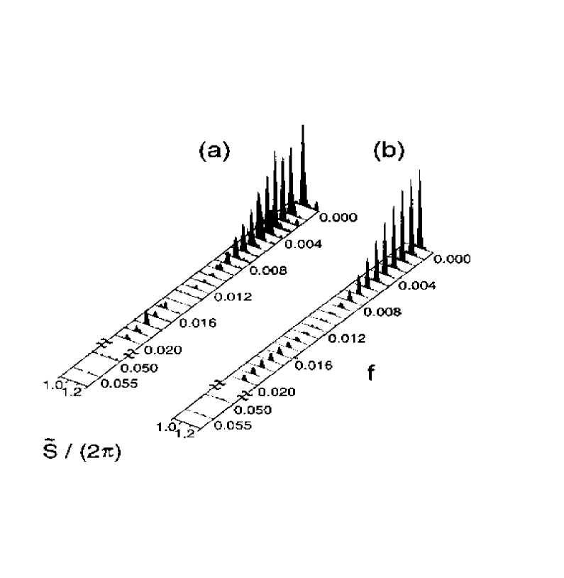
Figure 15: Segments of (a) experimental and (b) theoretical scaled action spectra for the hydrogen atom in crossed magnetic and electric fields at constant scaled energy $\tilde{E}=-0.15$. (From Ref. [54].)

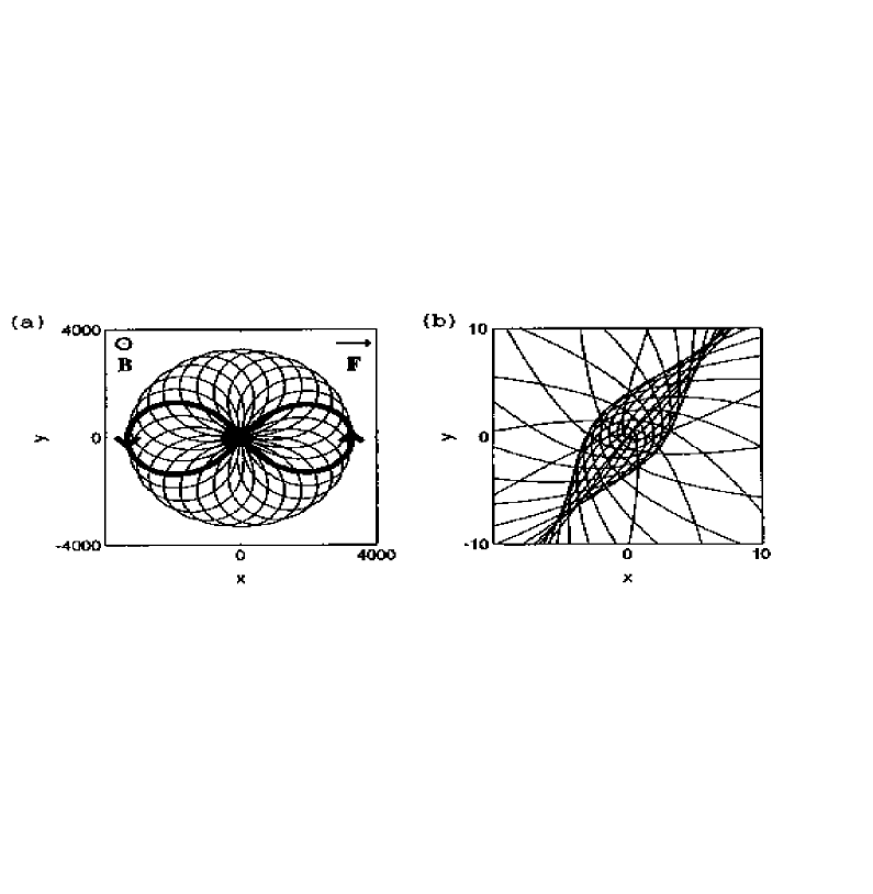
Figure 16: (a) Classical trajectories for the hydrogen atom in crossed fields in the plane perpendicular to the magnetic field axis. Scaled energy $\tilde{E}=-0.15$ and field strength $f=0.012$. (b) Closeup of the returning part of the trajectories as they approach the nucleus. (From Ref. [54].)

However, the expected splitting of recurrence peaks cannot be observed directly because of the finite resolution of the Fourier transform. This can be seen in Fig. 15 for the hydrogen atom in crossed fields. Fig. 15a presents segments of the experimental recurrence spectra at constant scaled energy $\tilde{E}=-0.15$ and scaled electric field strengths $0\leq f=F\gamma^{-4/3}\leq 0.055$. $F$ is the electric field strength in atomic units $(F_{0}=5.14\times 10^{9}\,{\rm V/cm})$. For comparison Fig. 15b shows the theoretical recurrence spectra obtained from semiclassical closed orbit theory [54]. Spectra have been Fourier transformed in the range $34.0\leq w=\gamma^{-1/3}\leq 61.7$. The recurrence structure corresponds to the classical orbit in the plane perpendicular to the magnetic field axis drawn in Fig. 16. At vanishing electric field trajectories starting at the origin are exactly closed at each return to the nucleus (thin line in Fig. 16a). For nonzero electric field, only two orbits with slightly different periods (shown with heavy lines in Fig. 16a) return exactly to the origin. A closeup of the returning part of the trajectories as they approach the nucleus at scaled energy $\tilde{E}=-0.15$ and field strength $f=0.012$ is given in Fig. 16b. The two closed orbits return to the nucleus diagonally; all others follow near-parabolic paths near the nucleus. In Fig. 15 no splitting of the recurrence peak can be observed due to the finite resolution of the Fourier transform spectra. However, the amplitude of the peak changes with increasing electric field strength, and indeed in Ref. [54] the symmetry breaking was identified indirectly by the constructive and destructive interference of the two orbits resulting in a Bessel function type modulation of amplitudes of recurrence peaks as a function of the strength of the symmetry breaking perturbation.

We now want to apply harmonic inversion to directly uncover the splitting of recurrence peaks when symmetries are broken. As in Ref. [54] we investigate the hydrogen atom in crossed magnetic and electric fields. Schrödinger’s equation for hydrogen in crossed fields reads

$$\left[{1\over 2}{\bf p}^{2}-{1\over r}+{1\over 2}\gamma L_{z}+{1\over 8}\gamma^{2}(x^{2}+y^{2})+Fx\right]\Psi=E\Psi\;,$$ (2.59)

with $\gamma$ and $F$ the magnetic and electric field strength (in atomic units), and $E$ the energy. The eigenvalue problem (2.59) was solved numerically for fixed external fields $\gamma$ and $F$ in Refs. [96, 105]. To study the effects of symmetry breaking on the quantum spectra we want to use the scaling properties of the classical system and to analyze spectra at constant scaled energy $\tilde{E}=E\gamma^{-2/3}$ and scaled electric field $f=F\gamma^{-4/3}$. Eigenvalues are obtained for the scaling parameter $w=\gamma^{-1/3}$. Introducing dilated coordinates $\bar{\bf r}=\gamma^{2/3}{\bf r}$ Eq. 2.59 reads

$$w^{2}\left[\bar{\bf p}^{2}\right]\Psi+w\left[L_{z}\right]\Psi+\left[{1\over 4}(\bar{x}^{2}+\bar{y}^{2})+2f\bar{x}-2\tilde{E}-{2\over\bar{r}}\right]\Psi=0\;.$$ (2.60)

The peculiarity of (2.60) is that it is a quadratic (instead of linear) eigenvalue equation for the scaling parameter $w$, which cannot be solved straightforwardly with standard diagonalization routines for linear eigenvalue problems. To solve the quadratic Schrödinger equation (2.60) we use the following technique. We write

$$w^{2}=\lambda=\lambda_{0}+\Delta\lambda\;,$$ (2.61)

with $\lambda_{0}$ fixed and assume that $\Delta\lambda$ is small. Now the scaling parameter $w$ in the paramagnetic term of (2.60) can be approximated by

$$w=\sqrt{\lambda}\approx\sqrt{\lambda_{0}}+{1\over 2\sqrt{\lambda_{0}}}\Delta\lambda\;.$$ (2.62)

Replacing $w$ in (2.60) with this approximation yields a generalized linear eigenvalue problem for $\Delta\lambda$,

$$\left[\lambda_{0}\bar{\bf p}^{2}+\sqrt{\lambda_{0}}L_{z}+{1\over 4}(\bar{x}^{2}+\bar{y}^{2})+2f\bar{x}-2\tilde{E}-{2\over\bar{r}}\right]\Psi$$ (2.63)

$$= -\Delta\lambda\left[\bar{\bf p}^{2}+{1\over 2\sqrt{\lambda_{0}}}L_{z}\right]\Psi\;,$$

which can be solved numerically with the Spectral Transformation Lanczos Method (STLM) [106]. The numerical details for the diagonalization of the linearized Schrödinger equation (2.63) in a complete set of Sturmian type basis functions are similar to the diagonalization of Eq. 2.59 at constant field strengths as described in [96]. It is convenient to choose identical parameters for both $\lambda_{0}$ and the center of the spectral transformation, so that the STLM method provides eigenvalues in the local neighborhood of $\lambda\approx\lambda_{0}$, i.e., $\Delta\lambda$ is small. However, the obtained eigenvalues are still not very precise because of the approximation (2.62). In a second step we therefore apply perturbation theory and use the eigenvectors $|\Psi\rangle$ of Eq. 2.63 to solve the quadratic equation (2.60) separately for each eigenvalue, $w_{n}$, in the corresponding one-dimensional subspace, i.e.

$$w_{n}^{2}\,\langle\Psi_{n}|\bar{\bf p}^{2}|\Psi_{n}\rangle+w_{n}\,\langle\Psi_{n}|L_{z}|\Psi_{n}\rangle$$

$${}+\langle\Psi_{n}|{1\over 4}(\bar{x}^{2}+\bar{y}^{2})+2f\bar{x}-2\tilde{E}-{2\over\bar{r}}|\Psi_{n}\rangle=0\;.$$ (2.64)

By this procedure the accuracy of the eigenvalues is significantly improved. An alternative method for the exact solution of the quadratic eigenvalue equation (2.60) is described in Ref. [107].

We now investigate the symmetry breaking in the hydrogen atom at constant scaled energy $\tilde{E}=-0.5$. Without electric field ($f=0$) the two shortest closed orbit recurrences are the perpendicular orbit at $s/2\pi=0.872$ and the parallel orbit at $s/2\pi=1$. When the cylindrical symmetry is broken by a crossed electric field, all three-dimensional orbits should split into two nearby peaks. The only exception is the orbit parallel to the magnetic field axis, which does not appear as a continuous family of closed orbits. To verify the symmetry breaking in quantum spectra we calculated the photoabsorption spectrum (transitions from the initial state $|2p0\rangle$ to the final states with even $z$-parity) up to $w=50$ for the crossed field atom at constant scaled energy $\tilde{E}=-0.5$ and scaled field strength $f=0.02$. The interesting part of the resulting recurrence spectrum obtained by both the conventional Fourier transform and the high resolution harmonic inversion technique are presented in Fig. 17. The conventional Fourier transform (smooth line) shows two peaks around $s/2\pi=0.87$ (the perpendicular orbit) and $s/2\pi=1$ (the parallel orbit). However, none of the peaks is split. The high resolution recurrence spectrum obtained by harmonic inversion is drawn as solid sticks and crosses in Fig. 17 and clearly exhibits a splitting of the recurrence peak of the perpendicular orbit at $s/2\pi\approx 0.87$. For comparison the semiclassical recurrence spectrum is presented as dashed sticks and squares. In the plane perpendicular to the magnetic field axis two closed orbits have been found with slightly different classical actions $s^{\rm cl}/2\pi=0.864$ and $s^{\rm cl}/2\pi=0.881$. The shapes of these orbits are illustrated as insets in Fig. 17. As can be seen the semiclassical and the high resolution quantum recurrence spectrum are in excellent agreement, i.e., the symmetry breaking in crossed fields has been directly uncovered by harmonic inversion of the quantum mechanical photoabsorption spectrum.

2.6 $\hbar$ expansion of the periodic orbit sum

In the previous sections we have introduced harmonic inversion as a powerful method for the high resolution analysis of quantum spectra, which allows a direct and quantitative comparison of the quantum spectra with semiclassical theories. However, the excellent agreement to many significant digits for both the periods and amplitudes of quantum mechanical recurrence peaks with the semiclassical periodic orbit contributions (see Section 2.3) may be surprising for the following reason. Periodic orbit theory is exact only for a special class of systems, e.g., the geodesic motion on a surface with constant negative curvature [8]. In general, the semiclassical periodic orbit sum is only the leading order contribution of an infinite series in powers of the Planck constant [22, 23, 24]. Therefore it might be expected that only the high resolution analysis of semiclassical spectra yields perfect agreement with periodic orbit theory while the harmonic inversion of quantum spectra should show small but noticeable deviations from the semiclassical recurrence spectra. As will be shown in the following, the absence of such deviations is related to the functional form of the $\hbar$ expansion of the periodic orbit sum and special properties of the harmonic inversion method.

In scaling systems, where the classical action of periodic orbits scales as

$$S_{\rm po}/\hbar=s_{\rm po}/\hbar_{\rm eff}=s_{\rm po}w\;,$$

the scaling parameter plays the role of an effective Planck constant, i.e.

$$w\equiv\hbar_{\rm eff}^{-1}\;,$$

and the $\hbar$ expansion of the periodic orbit sum can therefore be written as a power series in $w^{-1}$. The fluctuating part of the semiclassical response function is given by

$$g(w)=\sum_{n=0}^{\infty}g_{n}(w)=\sum_{n=0}^{\infty}{1\over w^{n}}\sum_{\rm po}{\cal A}_{\rm po}^{(n)}e^{is_{\rm po}w}\;.$$ (2.65)

The ${\cal A}_{\rm po}^{(n)}$ are the complex amplitudes of the $n^{\rm th}$ order periodic orbit contributions including phase information from the Maslov indices. When quantum spectra are analyzed in the semiclassical regime, i.e., at sufficiently high scaling parameter $w$, the higher order $\hbar$ correction terms $(n\geq 1)$ of the series (2.65) are certainly small compared to the zeroth order terms. However, the reason why the higher order contributions are not uncovered by the harmonic inversion method is that only the zeroth order $(n=0)$ terms in (2.65) fulfill the ansatz (2.14) required for harmonic inversion, i.e., they are exponential functions with constant frequencies and amplitudes. The higher order terms $(n\geq 1)$ have amplitudes decreasing $\sim w^{-n}$ with increasing scaling parameter, and thus do not fulfill the ansatz (2.14). Therefore only the zeroth order amplitudes ${\cal A}_{\rm po}^{(0)}$ can be obtained as converged parameters from the high resolution harmonic inversion analysis of the quantum spectra. The terms with $n\geq 1$ have similar properties as weak “noise” [70] and are separated by the harmonic inversion method from the “true” signal. In other words, the zeroth order approximation of the periodic orbit sum (2.65) with amplitudes ${\cal A}_{\rm po}^{(0)}$ given by Gutzwiller’s trace formula is the best fit to the quantum spectra within the given ansatz as a linear superposition of exponential functions of the scaling parameter $w$, and the corresponding parameters are obtained from the harmonic inversion procedure.

However, the higher order terms of the $\hbar$ expansion (2.65) can be revealed by harmonic inversion as will be demonstrated in the following. The periodic orbit terms ${\cal A}_{\rm po}^{(n)}$ can be obtained provided that the quantum spectrum and the $(n-1)^{\rm st}$ order eigenvalues $w_{k,n-1}$ are given. We can then calculate the difference between the exact quantum mechanical and the $(n-1)^{\rm st}$ order response function

$$g^{\rm qm}(w)-\sum_{j=0}^{n-1}g_{j}(w)=\sum_{j=n}^{\infty}g_{j}(w)=\sum_{j=n}^{\infty}{1\over w^{j}}\sum_{\rm po}{\cal A}_{\rm po}^{(j)}e^{is_{\rm po}w}\;.$$ (2.66)

The leading order terms in Eq. 2.66 are $\sim w^{-n}$, i.e., multiplication with $w^{n}$ yields

$$w^{n}\left[g^{\rm qm}(w)-\sum_{j=0}^{n-1}g_{j}(w)\right]=\sum_{\rm po}{\cal A}_{\rm po}^{(n)}e^{is_{\rm po}w}+{\cal O}\left({1\over w}\right)\;.$$ (2.67)

In Eq. 2.67 we have restored the functional form (2.14), i.e., a linear superposition of exponential functions of $w$. The harmonic inversion of the function (2.67) will now provide the periods $s_{\rm po}$ and the $n^{\rm th}$ order amplitudes ${\cal A}_{\rm po}^{(n)}$ of the $\hbar$ expansion (2.65). We will illustrate the method on two different examples, i.e., the circle billiard and the three disk scattering problem.

2.6.1 The circle billiard

The circle billiard is an integrable and even separable bound system, and has been chosen here mainly for the sake of simplicity, since all the relevant physical quantities, i.e., the quantum and semiclassical eigenenergies, and the periodic orbits can easily be obtained. In polar coordinates $(\rho,\phi)$ and after separation of the $\phi$-motion Schrödinger’s equation reads

$$-{\hbar^{2}\over 2M}\left({1\over\rho}{\partial\over\partial\rho}\rho{\partial\over\partial\rho}-{m^{2}\over\rho^{2}}\right)\Psi_{m}(\rho)=E\Psi_{m}(\rho)\;,$$ (2.68)

with $M$ the mass of the particle and $m$ the angular momentum quantum number. The wave functions must fulfill the boundary condition $\Psi_{m}(R)=0$ with $R$ the radius of the circle billiard. Defining

$$E={\hbar^{2}k^{2}\over 2M}$$

and after substitution of $z\equiv k\rho$ Schrödinger’s equation (2.68) is transformed into the differential equation for the Bessel functions [108]

$$z^{2}J_{m}^{\prime\prime}(z)+zJ_{m}^{\prime}(z)+(z^{2}-m^{2})J_{m}(z)=0\;.$$ (2.69)

The quantum mechanical eigenvalues $k_{n,m}^{\rm qm}$ are obtained from the boundary condition $J_{m}(k_{n,m}^{\rm qm}R)=0$ as zeros of the Bessel functions. We calculated numerically the first 32469 eigenenergies of the circle billiard in the region $k_{n,m}R<510$. Note that states with $m\neq 0$ are twofold degenerate.

The semiclassical eigenenergies are obtained from an EBK torus quantization or, after separation of the $\phi$-motion, even more simply from the one-dimensional WKB quantization of the radial motion in the centrifugal potential, i.e.

$$2\int_{m/k}^{R}p_{\rho}d\rho=2\hbar k\int_{m/k}^{R}\sqrt{1-(m/k\rho)^{2}}d\rho=2\pi\hbar\left(n+{3\over 4}\right)\;,$$ (2.70)

with $n=0,1,2,\dots$ the radial quantum number. The r.h.s. of Eq. 2.70 takes into account the correct boundary conditions of the semiclassical wave functions at the classical turning points. The zeroth order semiclassical eigenenergies are finally obtained from the quantization condition

$$kR\sqrt{1-(m/kR)^{2}}-|m|\arccos{|m|\over kR}=\pi\left(n+{3\over 4}\right)\;.$$ (2.71)

The semiclassical spectrum has been calculated with the help of Eq. 2.71 in the same region $k_{n,m}^{\rm sc}R<510$ as the exact quantum spectrum.

For the comparison of the spectra with periodic orbit theory we need to calculate the periodic orbits and their physical quantities. For the circle billiard all quantities are obtained analytically. In the following we choose $R=1$. The periodic orbits of the circle billiard are those orbits for which the angle between two bounces is a rational multiple of $2\pi$, i.e., the periods $\ell_{\rm po}$ are obtained from the condition

$$\ell_{\rm po}=2m_{r}\sin\gamma\;,$$ (2.72)

with

$$\gamma\equiv\pi{m_{\phi}\over m_{r}}\;,$$

$m_{\phi}=1,2,\dots$ the number of turns of the orbit around the origin, and $m_{r}=2m_{\phi},2m_{\phi}+1,\dots$ the number of reflections at the boundary of the circle. Periodic orbits with $m_{r}\neq 2m_{\phi}$ can be traversed in two directions and thus have multiplicity 2. Because the classical dynamics of the circle billiard is regular the Berry-Tabor formula [25] must be applied instead of Gutzwiller’s trace formula for the calculation of the semiclassical density of states. We obtain

$${1\over\sqrt{k}}g(k)={1\over\sqrt{k}}\sum_{n=0}^{\infty}g_{n}(k)=\sum_{n=0}^{\infty}{1\over k^{n}}\sum_{\rm po}{\cal A}_{\rm po}^{(n)}e^{i\ell_{\rm po}k}\;,$$ (2.73)

which basically differs from Eq. 2.65 by a factor of $k^{-1/2}$ on the l.h.s. of (2.73). [Note that for billiard systems the scaling parameter is the absolute value of the wave vector, $w\equiv k=|{\bf p}|/\hbar$, and the action is proportional to the length of the orbit, $S_{\rm po}=\hbar k\ell_{\rm po}$.] The zeroth order periodic orbit amplitudes obtained from the Berry-Tabor formula read

$${\cal A}_{\rm po}^{(0)}=\sqrt{\pi\over 2}{\ell_{\rm po}^{3/2}\over m_{r}^{2}}e^{-i({\pi\over 2}\mu_{\rm po}+{\pi\over 4})}\;,$$ (2.74)

with $\mu_{\rm po}=3m_{r}$ the Maslov index. For the calculation of the first order periodic orbit amplitudes ${\cal A}_{\rm po}^{(1)}$ in Eq. 2.73 we adopt the method of Alonso and Gaspard [23]. After a lengthy calculation we finally obtain

$${\cal A}_{\rm po}^{(1)}={1\over 2}\sqrt{\pi m_{r}}\,\underbrace{5-2\sin^{2}\gamma\over 3\sin^{3/2}\gamma}_{f(\gamma)}e^{-i({\pi\over 2}\mu_{\rm po}-{\pi\over 4})}\;.$$ (2.75)

A detailed derivation of Eqs. 2.74 and 2.75 will be given elsewhere [87, 88].

When the quantum mechanical density of states, or, more precisely, the spectrum $k^{-1/2}\varrho^{\rm qm}(k)$ is analyzed by the harmonic inversion method the periodic orbit quantities $\ell_{\rm po}$ and ${\cal A}_{\rm po}^{(0)}$ are obtained to very high precision [87]. However, we are now interested in the $\hbar$ expansion of the periodic orbit sum and want to verify the first order corrections ${\cal A}_{\rm po}^{(1)}$ directly in the quantum spectrum. We therefore analyze the difference spectrum $\Delta\varrho(k)=\varrho^{\rm qm}(k)-\varrho^{\rm sc}(k)$ between the quantum and the semiclassical density of states. A small part of this spectrum at $k\approx 200$ is presented in Fig. 18. The absolute values of the peak heights mark the multiplicities of the states. To restore the functional form which is required for the harmonic inversion procedure the difference spectrum was multiplied by $\sqrt{k}$, and the resulting signal $\sqrt{k}\Delta\varrho(k)$ was analyzed in the region $100<k<500$. The results are presented in Fig. 19. For a direct comparison with Eq. 2.75 we transform for each periodic orbit the obtained period $\ell_{\rm po}$ and the first order amplitude ${\cal A}_{\rm po}^{(1)}$ into the quantities

$$\gamma=\arcsin{\ell_{\rm po}\over 2m_{r}}\quad{\rm and}\quad f(\gamma)\equiv{2\over\sqrt{\pi m_{r}}}\,|{\cal A}_{\rm po}^{(1)}|\;.$$

These quantities are plotted as crosses in Fig. 19. The periodic orbits are marked by the numbers $(m_{\phi},m_{r})$. The solid line

$$f(\gamma)={5-2\sin^{2}\gamma\over 3\sin^{3/2}\gamma}$$

is the result of Eq. 2.75. As can be seen the theoretical curve and the crosses obtained by harmonic inversion of the difference between the quantum and semiclassical density of states are in excellent agreement.

The semiclassical accuracy of the zeroth order eigenenergies of the circle billiard has been discussed in Refs. [109, 110] in terms of, e.g., the average error in units of the mean level spacing. The analysis presented here provides a more physical interpretation of the deviations between the quantum and semiclassical eigenenergies in terms of the higher order corrections of the $\hbar$ expanded periodic orbit sum (2.65). The direct application of the series (2.65) for the semiclassical quantization beyond the Gutzwiller and Berry-Tabor approximation will be discussed in Section 3.6.

2.6.2 The three disk scattering system

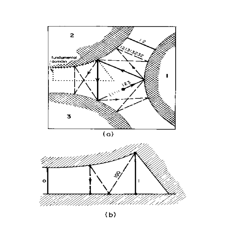
Figure 20: The scattering geometry for the three-disk system. (a) The three disks with 12, 123, and 121313232 cycles indicated. (b) The fundamental domain, i.e., a wedge consisting of a section of a disk, two segments of symmetry axis acting as straight mirror walls, and an escape gap. The above cycles restricted to the fundamental domain are now the 0, 1, and 100 cycle. (From Ref. [9].)

As a second example for the investigation of the $\hbar$ expansion of the periodic orbit sum we now consider a billiard system consisting of three identical hard disks with unit radius $R=1$, displaced from each other by the same distance, $d$. The classical, semiclassical, and quantum dynamics of this scattering system has been studied by Gaspard and Rice [111]. In recent years the system has served as a prototype model for periodic orbit quantization by cycle expansion techniques [9, 10, 11, 14, 15]. If the disks are separated by a distance $d>2.0481419$ there is a one-to-one identity between the periodic orbits and a symbolic code, whereas for $d<2.04821419$ pruning of orbits sets in [112]. The geometry of the three disk scattering system is shown in Fig. 20. The symbolic code of a periodic orbit is obtained by numbering of the disks, ’1’, ’2’, and ’3’, and by bookkeeping the reflections of the orbit at the three disks. E.g., $\overline{121313232}$ is the symbolic code of the primitive orbit with cycle length $n=9$ drawn with a dashed line in Fig. 20. The bar, which is often omitted, indicates the periodicity of the orbit. The three disk scattering system is invariant under the symmetry operations of the group $C_{3v}$, i.e., three reflections at symmetry lines and two rotations by $2\pi/3$ and $4\pi/3$. Periodic orbits have $\sigma_{v}$ symmetry if they are invariant under reflections and $C_{3},C_{3}^{2}$ symmetry if they are invariant under rotations. After symmetry decomposition the periodic orbits in the fundamental domain (see Fig. 20b) can be classified by a binary symbolic code of symbols ’0’ and ’1’, where each ’0’ represents a change between clockwise and anticlockwise scattering in the original three disk system [9]. The symbolic code of the orbit 121313232 in Fig. 20a restricted to the fundamental domain is 100100100 or because of its periodicity even simpler 100. The quantum resonances are also classified by symmetries. Resonances with $A_{1}$ ($A_{2}$) symmetry are symmetric (antisymmetric) under reflections at a symmetry line, and resonances with $E$ symmetry are invariant (up to a complex phase factor $c$ with $c^{3}=1$) under rotations by $2\pi/3$ and $4\pi/3$. The resonances in the $E$ subspace are twofold degenerate. In the following we analyze resonances with $A_{1}$ symmetry.

The three disk scattering system does not have any bound states. However, the fluctuating part of the density of states can be written as

$$\varrho(k)=-{1\over\pi}\,{\rm Im}\,\sum_{n}{1\over k-k_{n}}$$ (2.76)

with $k_{n}$ the complex resonances (poles) of the Green’s function. For distance $d=6$ the quantum mechanical $A_{1}$ resonances have been calculated by Wirzba [14, 15, 113] in the region $0<{\rm Re}~{}k<250$, and are plotted with the $+$ symbols in Fig. 21c. The corresponding fluctuating part of the quantum density of states is shown in Fig. 21a. This spectrum can be analyzed by harmonic inversion to extract the lengths (periods) of the orbits and the zeroth order amplitudes. However, as in the previous section for the circle billiard we here want to investigate the difference between the quantum and semiclassical spectrum. The semiclassical $A_{1}$ resonances have been calculated by Wirzba using the $12^{\rm th}$ order in the curvature expansion of the Gutzwiller-Voros zeta-function [14, 15, 113] and are plotted by the crosses $(\times)$ in Fig. 21c. The differences between the quantum and semiclassical resonances are usually much smaller than the size of the symbols in Fig. 21c and are visible only at small values of ${\rm Re}~{}k$. However, the deviations become clearly pronounced in Fig. 21b, which presents the difference between the quantum and zeroth order semiclassical density of states

$$k[\varrho^{\rm qm}(k)-\varrho^{\rm sc}(k)]=-{1\over\pi}\,{\rm Im}\,\sum_{\rm po}{\cal A}_{\rm po}^{(1)}e^{i\ell_{\rm po}k}+{\cal O}\left({1\over k}\right)\;.$$ (2.77)

Eq. 2.77 implies that by harmonic inversion of the spectrum in Fig. 21b we can extract the first order amplitudes ${\cal A}_{\rm po}^{(1)}$ of the $\hbar$ expansion of the periodic orbit sum. In Table 3 we present the ratio of the zeroth and first order amplitudes, $|{\cal A}_{\rm po}^{(1)}/{\cal A}_{\rm po}^{(0)}|^{\rm hi}$ obtained by harmonic inversion of the spectra in Fig. 21a and 21b for all periodic orbits up to cycle length 5 in the symmetry reduced symbolic code [9]. These quantities have been calculated by Alonso and Gaspard [23] and we present their results $|{\cal A}_{\rm po}^{(1)}/{\cal A}_{\rm po}^{(0)}|^{\rm cl}$ in Table 3 for comparison. In Ref. [23] the periodic orbits have not been symmetry reduced and the set of orbits chosen by Alonso and Gaspard is complete only up to cycle length 3 in the symmetry reduced symbolic code. However, Table 3 clearly illustrates a very good agreement between the amplitudes obtained by the harmonic inversion analysis of spectra and the results of Ref. [23].

We have here obtained information about the first order terms of the $\hbar$ expansion of the periodic orbit sum from the analysis of the quantum and the lowest (zeroth) order semiclassical resonances. In general, the quantum spectrum and its $n^{\rm th}$ order semiclassical approximation are required to extract information about the $(n+1)^{\rm st}$ order terms of the $\hbar$ expansion series (2.65).

3 Periodic orbit quantization by harmonic inversion

Since the development of periodic orbit theory by Gutzwiller [7, 8] it has become a fundamental question as to how individual semiclassical eigenenergies and resonances can be obtained from periodic orbit quantization for classically chaotic systems. A major problem is the exponential proliferation of the number of periodic orbits with increasing period, resulting in a divergence of Gutzwiller’s trace formula at real energies and below the real axis, where the poles of the Green’s function are located. The periodic orbit sum is a Dirichlet series

$$g(w)=\sum_{n}A_{n}e^{is_{n}w}\;,$$ (3.1)

where the parameters $A_{n}$ and $s_{n}$ are the amplitudes and periods (actions) of the periodic orbit contributions. In most applications Eq. 3.1 is absolutely convergent only in the region ${\rm Im}~{}w>c>0$ with $c$ the entropy barrier of the system, while the poles of $g(w)$, i.e., the bound states and resonances, are located on and below the real axis, ${\rm Im}~{}w\leq 0$. Thus, to extract individual eigenstates, the semiclassical trace formula (3.1) has to be analytically continued to the region of the quantum poles. Up to now no general procedure is known for the analytic continuation of a non-convergent Dirichlet series of the type of Eq. 3.1. All existing techniques are restricted to special situations. For bound and ergodic systems the semiclassical eigenenergies can be extracted with the help of a functional equation and the mean staircase function (Weyl term), resulting in a Riemann-Siegel look-alike formula [59, 60, 61]. Alternative semiclassical quantization conditions based on a semiclassical representation of the spectral staircase [65, 66] and derived from a quantum version of a classical Poincaré map [63] are also restricted to bound and ergodic systems. For systems with a symbolic dynamics the periodic orbit sum (3.1) can be reformulated as an infinite Euler product, which can be expanded in terms of the cycle length of the symbolic code. If the contributions of longer orbits are shadowed by the contributions of short orbits the cycle expansion technique can remarkably improve the convergence properties of the series and allows to extract the bound states and resonances of bound and open systems, respectively [9, 10, 11, 58]. A combination of the cycle expansion technique with a functional equation for bound systems has been studied by Tanner et al. [114]. However, the existence of a simple symbolic code is restricted to very few systems, and cycle expansion techniques cannot be applied, e.g., to the general class of systems with mixed regular-chaotic classical dynamics.

In this chapter we present a general technique for the analytic continuation and the extraction of poles of a non-convergent series of the type of Eq. 3.1. The method is based on harmonic inversion by filter-diagonalization. The advantage of the method is that it does not depend on special properties of the system such as ergodicity or the existence of a symbolic dynamics for periodic orbits. It does not even require the knowledge of the mean staircase function, i.e., the Weyl term in dynamical systems. The only assumption we have to make is that the analytic continuation of the Dirichlet series $g(w)$ (Eq. 3.1) is a linear combination of poles $(w-w_{k})^{-1}$, which is exactly the functional form of, e.g., a quantum mechanical response function with real and complex parameters $w_{k}$ representing the bound states and resonances of the system, respectively. To demonstrate the general applicability and accuracy of our method we will apply it to three systems with completely different properties, first the zeros of the Riemann zeta function [115, 116], as a mathematical model for a bound system, second the three disk scattering system as a physical example of an open system with classically chaotic dynamics, and third the circle billiard as an integrable system.

As pointed out by Berry [117] the density of zeros of Riemann’s zeta function can be written, in formal analogy with Gutzwiller’s semiclassical trace formula, as a non-convergent series, where the “periodic orbits” are the prime numbers. A special property of this system is the existence of a functional equation which allows the calculation of Riemann zeros via the Riemann-Siegel formula [115, 116, 117, 118]. An analogous functional equation for quantum systems with an underlying chaotic (ergodic) classical dynamics has served as the basis for the development of a semiclassical quantization rule for bound ergodic systems [59, 60, 61]. The Riemann zeta function has also served as a mathematical model to study the statistical properties of level distributions [118, 119, 120]. We will demonstrate in Section 3.1 that harmonic inversion can reveal the Riemann zeros with extremely high accuracy and with just prime numbers as input data. The most important advantage of our method is, however, its wide applicability, i.e., it can be generalized in a straightforward way to non-ergodic bound or open systems, and the procedure for periodic orbit quantization by harmonic inversion will be discussed in Section 3.2.

As an example of periodic orbit quantization of a physical system we investigate in Section 3.3 the three disk scattering problem, which is an open and non-ergodic system. Its classical dynamics is purely hyperbolic, and the periodic orbits can be classified by a complete binary symbolic code. This system has served as the prototype for the development of cycle expansion techniques [9, 10, 11]. When applying the harmonic inversion technique to the three disk scattering system we will highlight the general applicability of our method by not having to make use of its symbolic dynamics in any way.

The power of the method will be illustrated in Section 3.4 on a challenging physical system which has not been solved previously with any semiclassical quantization technique. The hydrogen atom in a magnetic field shows a transition from near-integrable to chaotic classical dynamics with increasing excitation energy. We apply periodic orbit quantization by harmonic inversion to the hydrogen atom in the mixed regular-chaotic regime.

An important question is the efficiency of methods for periodic orbit quantization, i.e., the number of periodic orbits required for the calculation of a certain number of poles of the response function $g(w)$. It is evident that methods invoking special properties of a given system may be remarkably efficient. E.g., the Riemann-Siegel type formulae [59, 60, 61] require the periodic orbits up to a maximum period which is by about a factor of four shorter compared to the required signal length for the harmonic inversion technique discussed in Section 3.2. We therefore propose in Section 3.5 an extension of the harmonic inversion method to the harmonic inversion of cross-correlated periodic orbit sums. The method uses additional semiclassical information obtained from a set of linearly independent smooth observables and allows to significantly reduce the number of periodic orbits and thus to improve the efficiency of periodic orbit quantization by harmonic inversion.

Periodic orbit theory yields exact eigenenergies only in exceptional cases, e.g., for the geodesic motion on the constant negative curvature surface [8]. As already discussed in Section 2.6, Gutzwiller’s periodic orbit sum is, in general, just the leading order term of an infinite series in powers of the Planck constant. Methods for the calculation of the higher order periodic orbit contributions were developed in [22, 23, 24]. In Section 3.6 we demonstrate how the higher order $\hbar$ corrections of the periodic orbit sum can be used to improve the accuracy of the semiclassical eigenenergies, i.e., to obtain eigenenergies beyond the standard semiclassical approximation of periodic orbit theory.

Both methods, the harmonic inversion of cross-correlated periodic orbit sums, which allows to significantly reduce the required number of periodic orbits for semiclassical quantization, and the calculation of eigenenergies beyond the lowest order $\hbar$ approximation will be illustrated in Section 3.7 by way of example of the circle billiard. Furthermore, for this system we will calculate semiclassically the diagonal matrix elements of various operators. The circle billiard is an integrable system and therefore the Berry-Tabor formula for integrable systems [25, 26] is valid in this case rather than Gutzwiller’s trace formula. However, periodic orbit quantization by harmonic inversion can be applied for both regular and chaotic systems as well which demonstrates the universality and wide applicability of the method.

Finally, in Section 3.8 we will calculate semiclassically the photoabsorption spectra of atoms in external fields. Applying a combination of closed orbit theory [90, 91, 92, 93], the cross-correlation approach of Section 3.5, and the harmonic inversion method we obtain individual non-diagonal transition matrix elements between low-lying initial states and strongly perturbed Rydberg states of the magnetized hydrogen atom.

3.1 A mathematical model: Riemann’s zeta function

Our goal is to introduce our method for periodic orbit quantization by harmonic inversion using, as an example, the well defined problem of calculating zeros of the Riemann zeta function. There are essentially two advantages of studying the zeta function instead of a “real” physical bound system. First, the Riemann analogue of Gutzwiller’s trace formula is exact, as is the case for systems with constant negative curvature [8, 66], whereas the semiclassical trace formula for systems with plane geometry is correct only to first order in $\hbar$. This allows a direct check on the precision of the method. Second, no extensive periodic orbit search is necessary for the calculation of Riemann zeros, as the only input data are just prime numbers. It is not our intention to introduce yet another method for computing Riemann zeros, which, as an objective in its own right, can be accomplished more efficiently by specific procedures. Rather, in our context the Riemann zeta function serves primarily as a mathematical model to illustrate the power of our technique when applied to bound systems.

3.1.1 General remarks

Before discussing the harmonic inversion method we start with recapitulating a few brief remarks on Riemann’s zeta function necessary for our purposes. The hypothesis of Riemann is that all the non-trivial zeros of the analytic continuation of the function

$$\zeta(z)=\sum_{n=1}^{\infty}n^{-z}=\prod_{p}\left(1-p^{-z}\right)^{-1}\;,\quad({\rm Re}~{}z>1,~{}p:{\rm primes})$$ (3.2)

have real part $1\over 2$, so that the values $w=w_{k}$, defined by

$$\zeta\left({1\over 2}-iw_{k}\right)=0,$$ (3.3)

are all real or purely imaginary [115, 116]. The Riemann staircase function for the zeros along the line $z={1\over 2}-iw$, defined as

$$N(w)=\sum_{k=1}^{\infty}\Theta(w-w_{k}),$$ (3.4)

i.e. the number $N(w)$ of zeros with $w_{k}<w$, can be split [115, 116, 117] into a smooth part,

$$\bar{N}(w) = {1\over\pi}\arg\Gamma\left({1\over 4}+{1\over 2}iw\right)-{w\over 2\pi}\ln\pi+1$$ (3.5)

$$= {w\over 2\pi}\left(\ln\left\{{w\over 2\pi}\right\}-1\right)+{7\over 8}+{1\over 48\pi w}-{7\over 5760\pi w^{3}}+{\cal O}(w^{-5})\;,$$

and a fluctuating part,

$$N_{\rm osc}(w)=-{1\over\pi}\lim_{\eta\to 0}\,{\rm Im}\,\ln\zeta\left({1\over 2}-i(w+i\eta)\right)\;.$$ (3.6)

Substituting the product formula (3.2) (assuming that it can be used when ${\rm Re}~{}z={1\over 2}$) into (3.6) and expanding the logarithms yields

$$N_{\rm osc}(w)=-{1\over\pi}\,{\rm Im}\,\sum_{p}\sum_{m=1}^{\infty}{1\over mp^{m/2}}\,e^{iwm\ln(p)}\;.$$ (3.7)

Therefore the density of zeros along the line $z={1\over 2}-iw$ can formally be written as

$$\varrho_{\rm osc}(w)=\frac{dN_{\rm osc}}{dw}=-{1\over\pi}\,{\rm Im}\,g(w)$$ (3.8)

with the response function $g(w)$ given by the series

$$g(w)=i\sum_{p}\sum_{m=1}^{\infty}\frac{\ln(p)}{p^{m/2}}\,e^{iwm\ln(p)}\ ,$$ (3.9)

which converges only for ${\rm Im}\,w>{1\over 2}$. Obviously Eq. 3.9 is of the same type as the response function (3.1), with the entropy barrier $c={1\over 2}$, i.e., Eq. 3.9 does not converge on the real axis, where the Riemann zeros are located. The mathematical analogy between the above equation and Gutzwiller’s periodic orbit sum

$$\varrho_{\rm osc}(E)\approx-{1\over\pi}\,{\rm Im}\,\sum_{\rm po}{\cal A}_{\rm po}\,e^{iS_{\rm po}},$$ (3.10)

with ${\cal A}_{\rm po}$ the amplitudes and $S_{\rm po}$ the classical actions (including phase information) of the periodic orbit contributions, was already pointed out by Berry [117, 59]. For the Riemann zeta function the primitive periodic orbits have to be identified with the primes $p$, and the integer $m$ formally counts the “repetitions” of orbits. The “amplitudes” and “actions” are then given by

$${\cal A}_{pm} = i{\ln(p)\over p^{m/2}}\;,$$ (3.11)

$$S_{pm} = mw\ln(p)\;.$$ (3.12)

Both equation (3.9) for the Riemann zeros and – for most classically chaotic physical systems – the periodic orbit sum (3.10) do not converge. In particular, zeros of the zeta function, or semiclassical eigenstates, cannot be obtained directly using these expressions. The problem is to find the analytic continuation of these equations to the region where the Riemann zeros or, for physical systems, the eigenenergies and resonances, are located. Eq. 3.9 is the starting point for our introduction and discussion of the harmonic inversion technique for the example of the Riemann zeta function. The generalization of the method to periodic orbit quantization (Eq. 3.10) in Section 3.2 will be straightforward.

Although Eq. 3.9 is the starting point for the harmonic inversion method, for completeness we quote the Riemann-Siegel formula, which is the most efficient approach to computing Riemann zeros. For the Riemann zeta function it follows from a functional equation [115] that the function

$$Z(w)=\exp\left\{-i\left[\arg\Gamma\left({1\over 4}+{1\over 2}iw\right)-{1\over 2}w\ln\pi\right]\right\}\zeta\left({1\over 2}-iw\right)$$ (3.13)

is real, and even for real $w$. The asymptotic representation of $Z(w)$ for large $w$,

$$Z(w) = -2\sum_{n=1}^{{\rm Int}[\sqrt{w/2\pi}]}\frac{\cos\{\pi\bar{N}(w)-w\ln n\}}{n^{1/2}}$$ (3.14)

$$- (-1)^{{\rm Int}[\sqrt{w/2\pi}]}\left({2\pi\over w}\right)^{1\over 4}\;{\cos\left(2\pi\left(t^{2}-t-{1/16}\right)\right)\over\cos\left(2\pi t\right)}+\dots\;,$$

with $t=\sqrt{w/2\pi}-{\rm Int}[\sqrt{w/2\pi}]$ is known as the Riemann-Siegel formula and has been employed (with several more correction terms) in effective methods for computing Riemann zeros [118]. Note that the principal sum in (3.14) has discontinuities at integer positions of $\sqrt{w/2\pi}$, and therefore the Riemann zeros obtained from the principal sum are correct only to about 1 to 15 percent of the mean spacing between the zeros. The higher order corrections to the principal Riemann-Siegel sum remove, one by one, the discontinuities in successive derivatives of $Z(w)$ at the truncation points and are thus essential to obtaining accurate numerical results. An alternative method for improving the asymptotic representation of $Z(w)$ by smoothing the cutoffs with an error function and adding higher order correction terms is presented in [61]. An analogue of the functional equation for bound and ergodic dynamical systems has been used as the starting point to develop a “rule for quantizing chaos” via a “Riemann-Siegel look-alike formula” [59, 60, 61]. This method is very efficient as it requires the least number of periodic orbits, but unfortunately it is restricted to ergodic systems on principle reasons, and cannot be generalized either to systems with regular or mixed classical dynamics or to open systems. By contrast, the method of harmonic inversion does not have these restrictions. We will demonstrate that Riemann zeros can be obtained directly from the ”ingredients” of the non-convergent response function (3.9), i.e., the set of values $A_{pm}$ and $S_{pm}$, thus avoiding the use of the functional equation, the Riemann-Siegel formula, the mean staircase function (3.5), or any other special property of the zeta function. The comparison of results in Section 3.1.3 will show that the accuracy of our method goes far beyond the Riemann-Siegel formula (3.14) without higher order correction terms. The main goal of this section is to demonstrate that because of the formal equivalence between Eqs. (3.9) and (3.10) our method can then be applied to periodic orbit quantization of dynamical systems in Section 3.2 without any modification.

3.1.2 The ansatz for the Riemann zeros

To find the analytic continuation of Eq. (3.9) in the region ${\rm Im}~{}w<{1\over 2}$ we essentially wish to fit $g(w)$ to its exact functional form,

$$g_{\rm ex}(w)=\sum_{k}{d_{k}\over w-w_{k}+i0}\;,$$ (3.15)

arising from the definition of the Riemann staircase (3.4). The “multiplicities” $d_{k}$ in Eq. 3.15 are formally fitting parameters, which here should all be equal to 1. It is hard to directly adjust the non-convergent (on the real axis) series $g(w)$ to the form of $g_{\rm ex}(w)$. The first step towards the solution of the problem is to carry out the adjustment for the Fourier components of the response function,

$$C(s)={1\over 2\pi}\int_{-\infty}^{+\infty}g(w)e^{-isw}dw=i\sum_{p}\sum_{m=1}^{\infty}\frac{\ln(p)}{p^{m/2}}\,\delta(s-m\ln(p))\,,$$ (3.16)

which after certain regularizations (see below) is a well-behaved function of $s$. Due to the formal analogy with the results of periodic orbit theory (see Eqs. 3.11 and 3.12), $C(s)$ can be interpreted as the recurrence function for the Riemann zeta function, with the recurrence positions $s_{pm}=S_{pm}/w=m\ln(p)$ and recurrence strengths of periodic orbit returns $A_{pm}=i\ln(p)p^{-m/2}$. The exact functional form which now should be used to adjust $C(s)$ is given by

$$C_{\rm ex}(s)={1\over 2\pi}\int_{-\infty}^{+\infty}g_{\rm ex}(w)e^{-isw}dw=-i\sum_{k=1}^{\infty}d_{k}e^{-iw_{k}s}\;.$$ (3.17)

$C_{\rm ex}(s)$ is a superposition of sinusoidal functions with frequencies $w_{k}$ given by the Riemann zeros and amplitudes $d_{k}=1$. (It is convenient to use the word “frequencies” for $w_{k}$ referring to the sinusoidal form of $C(s)$. We will also use the word “poles” in the context of the response function $g(w)$.)

Fitting a signal $C(s)$ to the functional form of Eq. 3.17 with, in general, both complex frequencies $w_{k}$ and amplitudes $d_{k}$ is known as harmonic inversion, and has already been introduced in Section 2.2 for the high resolution analysis of quantum spectra. The harmonic inversion analysis is especially non-trivial if the number of frequencies in the signal $C(s)$ is large, e.g., more than a thousand. It is additionally complicated by the fact that the conventional way to perform the spectral analysis by studying the Fourier spectrum of $C(s)$ will bring us back to analyzing the non-convergent response function $g(w)$ defined in Eq. 3.9. Until recently the known techniques of spectral analysis [67] would not be applicable in the present case, and it is the filter-diagonalization method [68, 69, 70] which has turned the harmonic inversion concept into a general and powerful computational tool.

The signal $C(s)$ as defined by Eq. 3.16 is not yet suitable for the spectral analysis. The next step is to regularize $C(s)$ by convoluting it with a Gaussian function to obtain the smoothed signal,

$$C_{\sigma}(s) = {1\over\sqrt{2\pi}\sigma}\int_{-\infty}^{+\infty}C(s^{\prime})e^{-(s-s^{\prime})^{2}/2\sigma^{2}}ds^{\prime}$$ (3.18)

$$= {i\over\sqrt{2\pi}\sigma}\sum_{p}\sum_{m=1}^{\infty}{\ln(p)\over p^{m/2}}\,e^{-(s-m\ln(p))^{2}/2\sigma^{2}}$$

that has to be adjusted to the functional form of the corresponding convolution of $C_{\rm ex}(s)$. The latter is readily obtained by substituting $d_{k}$ in Eq. 3.17 by the damped amplitudes,

$$d_{k}\to d_{k}^{(\sigma)}=d_{k}\,e^{-w_{k}^{2}\sigma^{2}/2}\;.$$ (3.19)

The regularization (3.18) can also be interpreted as a cut of an infinite number of high frequencies in the signal which is of fundamental importance for numerically stable harmonic inversion. Note that the convolution with the Gaussian function is no approximation, and the obtained frequencies $w_{k}$ and amplitudes $d_{k}$ corrected by Eq. 3.19 are still exact, i.e., do not depend on $\sigma$. The convolution is therefore not related to the Gaussian smoothing devised for Riemann zeros in [121] and for quantum mechanics in [122], which provides low resolution spectra only.

The next step is to analyze the signal (3.18) by harmonic inversion. The concept of harmonic inversion by filter-diagonalization has already been explained in Section 2.2 and the technical details are given in Appendix A.1. Note that even though the derivation of Eq. 3.18 assumed that the zeros $w_{k}$ are on the real axis, the analytic properties of $C_{\sigma}(s)$ imply that its representation by Eq. 3.18 includes not only the non-trivial real zeros, but also all the trivial ones, $w_{k}=-i(2k+{1\over 2})$, $k=1,2,\dots$, which are purely imaginary. The general harmonic inversion procedure does not require the frequencies to be real. Both the real and imaginary zeros $w_{k}$ will be obtained as the eigenvalues of the non-Hermitian generalized eigenvalue problem, Eq. 1.7 in Appendix A.1.

3.1.3 Numerical results

For a numerical demonstration we construct the signal $C_{\sigma}(s)$ using Eq. 3.18 in the region $s<\ln(10^{6})=13.82$ from the first 78498 prime numbers and with a Gaussian smoothing width $\sigma=0.0003$. Parts of the signal are presented in Fig. 22. Up to $s\approx 8$ the Gaussian approximations to the $\delta$-functions do essentially not overlap (see Fig. 22a) whereas for $s\gg 8$ the mean spacing $\Delta s$ between successive $\delta$-functions becomes much less than the Gaussian width $\sigma=0.0003$ and the signal fluctuates around the mean $\bar{C}(s)=ie^{s/2}$ (see Fig. 22b). From this signal we were able to calculate about 2600 Riemann zeros to at least 12 digit precision. For the small generalized eigenvalue problem (see Eq. 1.7 in Appendix A.1) we used matrices with dimension $J<100$. Some Riemann zeros $w_{k}$, the corresponding amplitudes $d_{k}$, and the estimated errors $\varepsilon$ (see Eq. 1.12 in Appendix A.1) are given in Tables 4 and 5. The pole of the zeta function yields the smooth background $\bar{C}(s)=ie^{s/2}$ of the signal $C(s)$ (see the dashed line in Fig. 22). Within the numerical error the Riemann zeros are real and the amplitudes are consistent with $d_{k}=1$ for non-degenerate zeros. To fully appreciate the accuracy of our harmonic inversion technique we note that zeros obtained from the principal sum of the Riemann-Siegel formula (3.14) deviate by about 1 to 15 percent of the mean spacing from the exact zeros. Including the first correction term in (3.14) the approximations to the first five zeros read $w_{1}=14.137$, $w_{2}=21.024$, $w_{3}=25.018$, $w_{4}=30.428$, and $w_{5}=32.933$, which still significantly deviates from the exact values (see Table 4). Considering even higher order correction terms the results will certainly converge to the exact zeros. However, the generalization of such higher order corrections to ergodic dynamical systems is a nontrivial task and requires, e.g., the knowledge of the terms in the Weyl series, i.e., the mean staircase function after the constant [61, 123]. The perfect agreement of our results for the $w_{k}$ with the exact Riemann zeros to full numerical precision is remarkable and clearly demonstrates that harmonic inversion by filter-diagonalization is a very powerful and accurate technique for the analytic continuation and the extraction of poles of a non-convergent series such as Eq. 3.1.

A few $w_{k}$ have been obtained (see Table 6) which are definitely not located on the real axis. Except for the first at $w=i/2$ they can be identified with the trivial real zeros of the zeta function at $z=-2n$; $n=1,2,\dots$ In contrast to the nontrivial zeros with real $w_{k}$, the numerical accuracy for the trivial zeros decreases rapidly with increasing $n$. The trivial zeros $w_{n}=-i(2n+{1\over 2})$ are the analogue of resonances in open physical systems with widths increasing with $n$. The fact that the trivial Riemann zeros are obtained emphasizes the universality of our method and demonstrates that periodic orbit quantization by harmonic inversion can be applied not only to closed but to open systems as well. The decrease of the numerical accuracy for very broad resonances is a natural numerical consequence of the harmonic inversion procedure [69, 70]. The value $w=i/2$ in Table 6 is special because in this case the amplitude is negative, i.e., $d_{k}=-1$. Writing the zeta function in the form [116]

$$\zeta({1\over 2}-iw)=C\prod_{k}(w-w_{k})^{d_{k}}A(w,w_{k})$$ (3.20)

where $C$ is a constant and $A$ a regularizing function which ensures convergence of the product, integer values $d_{k}$ are the multiplicities of zeros. Therefore it is reasonable to relate negative integer values with the multiplicities of poles. In fact, $\zeta(z)$ has a simple pole at $z={1\over 2}-iw=1$ consistent with $w=i/2$ in Table 6.

3.1.4 Required signal length

We have calculated Riemann zeros by harmonic inversion of the signal $C_{\sigma}(s)$ (Eq. 3.18) which uses prime numbers as input. The question arises what are the requirements on the signal $C_{\sigma}(s)$, in particular what is the required signal length. In other words, how many Riemann zeros (or semiclassical eigenenergies) can be converged for a given set of prime numbers (or periodic orbits, respectively)? The answer can be directly obtained from the requirements on the harmonic inversion technique. In general, the required signal length $s_{\rm max}$ for harmonic inversion is related to the average density of frequencies $\bar{\varrho}(w)$ by [70]

$$s_{\rm max}\approx 4\pi\bar{\varrho}(w)\;,$$ (3.21)

i.e., $s_{\rm max}$ is about two times the Heisenberg length

$$s_{\rm Heisenberg}\equiv 2\pi\bar{\varrho}(w)\;.$$ (3.22)

From Eq. 3.21 the required number of primes (or periodic orbits) can be directly estimated as $\{\#~{}{\rm primes}~{}p~{}|~{}\ln p<s_{\rm max}\}$ or $\{\#~{}{\rm periodic~{}orbits}~{}|~{}s_{\rm po}<s_{\rm max}\}$. For the special example of the Riemann zeta function the required number of primes to have a given number of Riemann zeros converged can be estimated analytically. With the average density of Riemann zeros derived from (3.5),

$$\bar{\varrho}(w)=\frac{d\bar{N}}{dw}={1\over 2\pi}\ln\left({w\over 2\pi}\right)\;,$$ (3.23)

we obtain

$$s_{\rm max}=\ln(p_{\rm max})=2\ln\left({w\over 2\pi}\right)\Rightarrow p_{\rm max}=\left({w\over 2\pi}\right)^{2}\;.$$ (3.24)

The number of primes with $p<p_{\rm max}$ can be estimated from the prime number theorem

$$\pi(p_{\rm max})\sim\frac{p_{\rm max}}{\ln(p_{\rm max})}=\frac{(w/2\pi)^{2}}{2\ln(w/2\pi)}\;.$$ (3.25)

On the other hand the number of Riemann zeros as a function of $w$ is given by Eq. (3.5). The estimated number of Riemann zeros which can be obtained by harmonic inversion from a given set of primes is presented in Fig. 23. For example, about 80 zeros $(w<200)$ can be extracted from the short signal $C_{\sigma}(s)$ with $s_{\rm max}=\ln(1000)=6.91$ (168 prime numbers) in agreement with the estimates given above. Obviously, in the special case of the Riemann zeta function the efficiency of our method cannot compete with that of the Riemann-Siegel formula method (3.14) where the number of terms is given by $n_{\rm max}={\rm Int}\,[\sqrt{w/2\pi}]$ and, e.g., 5 terms in Eq. 3.14 would be sufficient to calculate good approximations to the Riemann zeros in the region $w<200$. Our primary intention is to introduce harmonic inversion by way of example of the zeros of the Riemann zeta function as a universal tool for periodic orbit quantization, and not to use it as an alternative method for solving the problem of finding most efficiently zeros of the Riemann zeta function. For the semiclassical quantization of bound and ergodic systems a functional equation can be invoked to derive a Riemann-Siegel look-alike quantization condition [59, 60, 61]. In this case the required number of periodic orbits can be estimated from the condition

$$s_{\rm max}\approx\pi\bar{\varrho}(w)={1\over 2}s_{\rm Heisenberg}\;,$$ (3.26)

which differs by a factor of 4 from the required signal length (3.21) for harmonic inversion. Obviously, the limitation (3.21) is unfavorable for periodic orbit quantization because of the exponential proliferation of the number of orbits in chaotic systems, and methods for a significant reduction of the signal length $s_{\rm max}$ are highly desirable. In fact, this can be achieved by an extension of the harmonic inversion technique to cross-correlation signals. We will return to this problem in Section 3.5.

3.2 Periodic orbit quantization

As mentioned in Section 3.1 the basic equation (3.9) used for the calculation of Riemann zeros has the same mathematical form as Gutzwiller’s semiclassical trace formula. Both series, Eq. 3.9 and the periodic orbit sum (3.10), suffer from similar convergence problems in that they are absolutely convergent only in the complex half-plane outside the region where the Riemann zeros, or quantum eigenvalues, respectively, are located. As a consequence, in a direct summation of periodic orbit contributions smoothing techniques must be applied resulting in low resolution spectra for the density of states [78, 122]. To extract individual eigenstates the semiclassical trace formula has to be analytically continued to the region of the quantum poles, and this was the subject of intense research during recent years.

For strongly chaotic bound systems a semiclassical quantization condition based on a semiclassical representation of the spectral staircase

$${\cal N}(E)=\sum_{n}\Theta(E-E_{n})$$ (3.27)

has been developed by Aurich et al. in Refs. [65, 66]. They suggest to replace the spectral staircase ${\cal N}(E)$ with a smooth semiclassical approximation ${\cal N}_{\rm sc}(E)$, and to evaluate the semiclassical eigenenergies from the quantization condition

$$\cos\left\{\pi{\cal N}_{\rm sc}(E)\right\}=0\;.$$ (3.28)

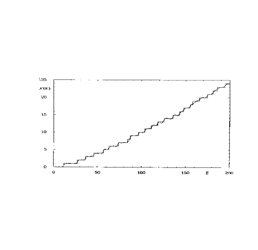
Figure 24: The spectral staircase ${\cal N}^{+}(E)$ and its semiclassical approximation ${\cal N}^{+}_{\rm sc}(E)$ for the hyperbolic billiard. ${\cal N}^{+}_{\rm sc}(E)$ was calculated using 101265 periodic orbits. (From Ref. [65].)

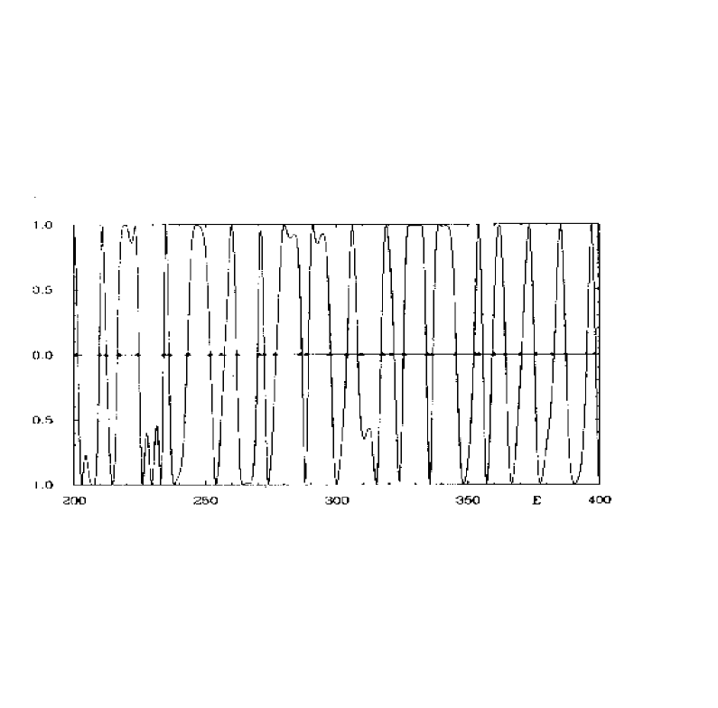
Figure 25: The function $\cos\{\pi{\cal N}^{+}_{\rm sc}(E)\}$ for the hyperbolic billiard. ${\cal N}^{+}_{\rm sc}(E)$ was evaluated as in Fig. 24. The triangles mark the positions of the true quantum mechanical energies. (From Ref. [65].)

For the even parity states of the hyperbola billiard the exact spectral staircase ${\cal N}^{+}(E)$ and the semiclassical approximation ${\cal N}^{+}_{\rm sc}(E)$ evaluated from 101265 periodic orbits are shown in Fig. 24. The function $\cos\left\{\pi{\cal N}^{+}_{\rm sc}(E)\right\}$ obtained from the smooth spectral staircase ${\cal N}^{+}_{\rm sc}(E)$ in Fig. 24 is presented in Fig. 25. According to the quantization condition (3.28) the zeros of this function are the semiclassical energies, and are in good agreement with the true quantum mechanical energies marked by triangles in Fig. 25. The quantization condition (3.28) was also successfully applied to the motion of a particle on various Riemann surfaces with constant negative curvature, e.g., Artin’s billiard or the Hadamard-Gutzwiller model [65, 66]. Another technique for bound and ergodic systems is to apply an approximate functional equation and generalize the Riemann-Siegel formula (3.14) to dynamical zeta functions [59, 60, 61]. The Riemann-Siegel look-alike formula has been applied, e.g., for the semiclassical quantization of the hyperbola billiard [123].

These quantization techniques cannot be applied to open systems. However, if a symbolic dynamics for the system exists, i.e., if the periodic orbits can be classified with the help of a complete symbolic code, the dynamical zeta function, given as an infinite Euler product over entries from classical periodic orbits, can be expanded in terms of the cycle length of the orbits [9, 58]. The cycle expansion series is rapidly convergent if the contributions of long orbits are approximately shadowed by contributions of short orbits. The cycle expansion technique has been applied, e.g., to the three disk scattering system [9, 10, 11] (see also Section 3.3), the three body Coulomb system [6, 124], and to the hydrogen atom in a magnetic field [20].

It turns out that the cycle expansion of dynamical zeta functions converges very slowly for bound systems. Therefore, a combination of the cycle expansion method with a functional equation has been developed by Tanner et al. [114, 125]. Applying a functional equation to the dynamical zeta function they conclude that the zeros of the real expression

$$D(E)=e^{-i\pi\bar{\cal N}(E)}Z(E)+e^{i\pi\bar{\cal N}(E)}Z^{\ast}(E)\;,$$ (3.29)

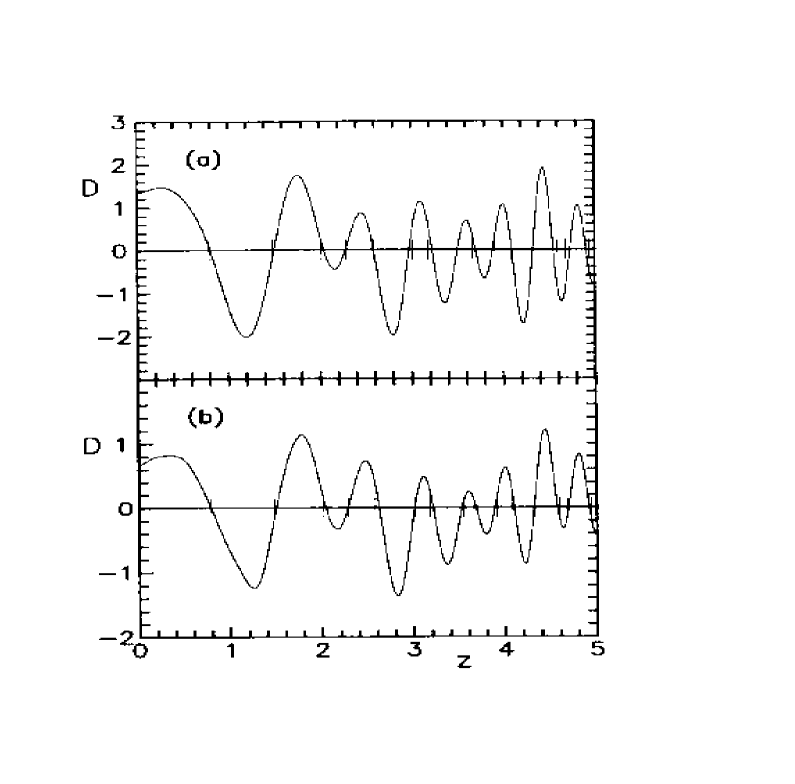
Figure 26: The cycle-expanded functional determinant for the $m^{\pi}=0^{+}$ subspace of the anisotropic Kepler problem. The quantum eigenvalues are marked with vertical bars on the real axis. (a) All orbits up to length 4 (8 in number) included. (b) All orbits up to length 8 (71) included. (From Ref. [114].)

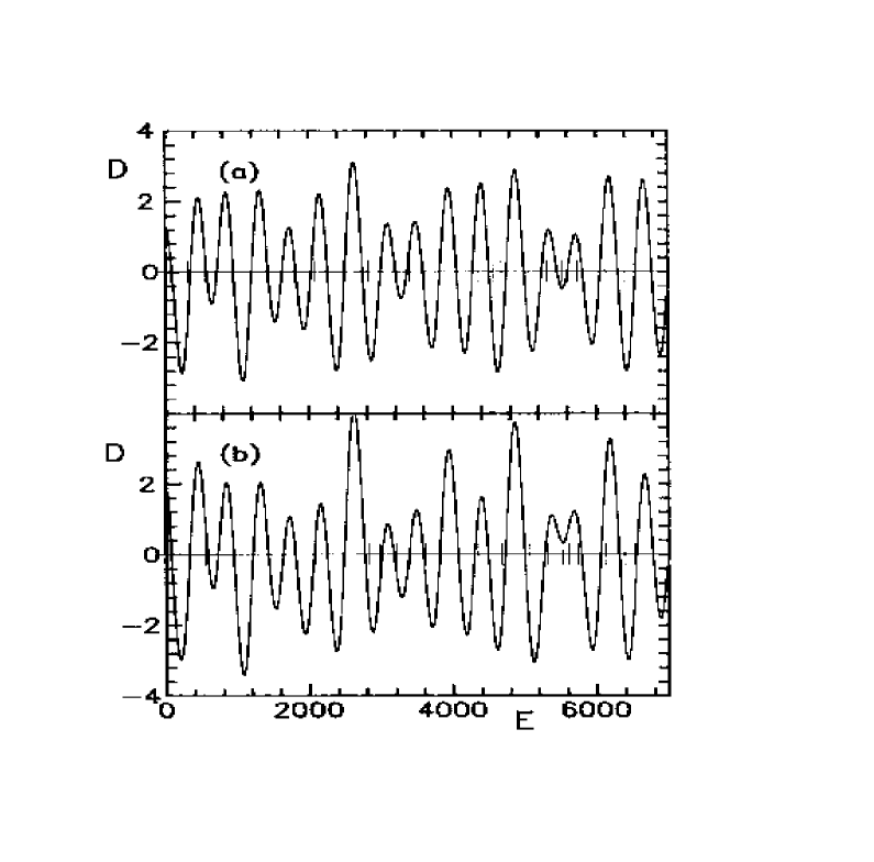
Figure 27: The cycle-expanded functional determinant for the closed three disk billiard (disk radius $R=1$). The vertical bars mark the exact quantum eigenvalues. (a) All orbits up to length 2 (3 in number) included. (b) All orbits up to length 3 (5) included. (From Ref. [114].)

with $\bar{\cal N}(E)$ the mean spectral staircase and $Z(E)$ the cycle expanded dynamical zeta function should be semiclassical approximations to the eigenvalues. The semiclassical functional determinant $D(E)$ is illustrated in Fig. 26 for the anisotropic Kepler problem [8] and in Fig. 27 for the closed three disk billiard, i.e., the system shown in Fig. 20 with touching disks. The vertical bars in Figs. 26 and 27 mark the exact eigenvalues.

The existence of a complete symbolic dynamics is more the exception than the rule, and therefore cycle expansion techniques cannot be applied, in particular, for systems with mixed regular-chaotic classical dynamics. In this section we apply the same technique that we used for the calculation of Riemann zeros to the calculation of semiclassical eigenenergies and resonances of physical systems by harmonic inversion of Gutzwiller’s periodic orbit sum for the propagator. The method only requires the knowledge of all orbits up to a sufficiently long but finite period and does neither rely on an approximate semiclassical functional equation, nor on the existence of a symbolic code for the orbits. The universality of the method will therefore allow the investigation of a large variety of systems with an underlying chaotic, regular, or even mixed classical dynamics. The derivation of an expression for the recurrence function to be harmonically inverted is analogous to that in Section 3.1.2.

3.2.1 Semiclassical density of states

Following Gutzwiller [7, 8] the semiclassical response function for chaotic systems is given by

$$g^{\rm sc}(E)=g^{\rm sc}_{0}(E)+\sum_{\rm po}{\cal A}_{\rm po}e^{iS_{\rm po}}\;,$$ (3.30)

where $g^{\rm sc}_{0}(E)$ is a smooth function and the $S_{\rm po}$ and ${\cal A}_{\rm po}$ are the classical actions and weights (including phase information given by the Maslov index) of periodic orbit contributions. Eq. (3.30) is also valid for integrable [25, 26] and near-integrable [27, 28] systems but with different expressions for the amplitudes ${\cal A}_{\rm po}$. It should also be possible to include complex “ghost” orbits [36, 37] and uniform semiclassical approximations [40, 44] close to bifurcations of periodic orbits in the semiclassical response function (3.30). The eigenenergies and resonances are the poles of the response function but, unfortunately, its semiclassical approximation (3.30) does not converge in the region of the poles, whence the problem is the analytic continuation of $g^{\rm sc}(E)$ to this region.

In the following we make the (weak) assumption that the classical system has a scaling property (see Section 2.1), i.e., the shape of periodic orbits does not depend on the scaling parameter, $w$, and the classical action scales as

$$S_{\rm po}=ws_{\rm po}\;.$$ (3.31)

Examples of scaling systems are billiards [9, 16], Hamiltonians with homogeneous potentials [126, 127], Coulomb systems [6], or the hydrogen atom in external magnetic and electric fields [47, 20]. Eq. 3.31 can even be applied for non-scaling, e.g., molecular systems if a generalized scaling parameter $w\equiv\hbar_{\rm eff}^{-1}$ is introduced as a new dynamical variable [94]. Quantization yields bound states or resonances, $w_{k}$, for the scaling parameter. In scaling systems the semiclassical response function $g^{\rm sc}(w)$ can be Fourier transformed easily to obtain the semiclassical trace of the propagator

$$C^{\rm sc}(s)={1\over 2\pi}\int_{-\infty}^{+\infty}g^{\rm sc}(w)e^{-isw}dw=\sum_{\rm po}{\cal A}_{\rm po}\delta\left(s-s_{\rm po}\right)\;.$$ (3.32)

The signal $C^{\rm sc}(s)$ has $\delta$-peaks at the positions of the classical periods (scaled actions) $s=s_{\rm po}$ of periodic orbits and with peak heights (recurrence strengths) ${\cal A}_{\rm po}$, i.e., $C^{\rm sc}(s)$ is Gutzwiller’s periodic orbit recurrence function. Consider now the quantum mechanical counterparts of $g^{\rm sc}(w)$ and $C^{\rm sc}(w)$ taken as the sums over the poles $w_{k}$ of the Green’s function,

$$g^{\rm qm}(w)=\sum_{k}{d_{k}\over w-w_{k}+i0}\;,$$ (3.33)

$$C^{\rm qm}(s)={1\over 2\pi}\int_{-\infty}^{+\infty}g^{\rm qm}(w)e^{-isw}dw=-i\sum_{k}d_{k}e^{-iw_{k}s}\;,$$ (3.34)

with $d_{k}$ being the multiplicities of resonances, i.e., $d_{k}=1$ for non-degenerate states. In analogy with the calculation of Riemann zeros from Eq. (3.18) the frequencies, $w_{k}$, and amplitudes, $d_{k}$, can be extracted by harmonic inversion of the signal $C^{\rm sc}(s)$ after convoluting it with a Gaussian function, i.e.,

$$C_{\sigma}^{\rm sc}(s)={1\over\sqrt{2\pi}\sigma}\sum_{\rm po}{\cal A}_{\rm po}e^{(s-s_{\rm po})^{2}/2\sigma^{2}}\;.$$ (3.35)

By adjusting $C_{\sigma}^{\rm sc}(s)$ to the functional form of Eq. 3.34, the frequencies, $w_{k}$, can be interpreted as the semiclassical approximation to the poles of the Green’s function in (3.33). Note that the harmonic inversion method described in Appendix A.1 allows studying signals with complex frequencies $w_{k}$ as well. For open systems the complex frequencies can be interpreted as semiclassical resonances. Note also that the $w_{k}$ in general differ from the exact quantum eigenvalues because Gutzwiller’s trace formula (3.30) is an approximation, correct only to the lowest order in $\hbar$. Therefore the diagonalization of small matrices (Eq. 1.7 in Appendix A.1) does not imply that the results of the periodic orbit quantization are more “quantum” in any sense than those obtained, e.g., from a cycle expansion [9, 58]. However, the harmonic inversion technique also allows the calculation of higher order $\hbar$ corrections to the periodic orbit sum, and we will return to this problem in Section 3.6.

3.2.2 Semiclassical matrix elements

The procedure described above can be generalized in a straightforward manner to the calculation of semiclassical diagonal matrix elements $\langle\psi_{k}|\hat{A}|\psi_{k}\rangle$ of a smooth Hermitian operator $\hat{A}$. In this case we start from the quantum mechanical trace formula

$$g_{A}^{\rm qm}(w)={\rm tr}\,G^{+}\hat{A}=\sum_{k}{\langle\psi_{k}|\hat{A}|\psi_{k}\rangle\over w-w_{k}+i0}\;,$$ (3.36)

which has the same functional form as (3.33), but with $d_{k}=\langle\psi_{k}|\hat{A}|\psi_{k}\rangle$ instead of $d_{k}=1$. For the quantum response function $g_{A}^{\rm qm}(w)$ (Eq. 3.36) a semiclassical approximation has been derived in [128, 129], which has the same form as Gutzwiller’s trace formula (3.30) but with amplitudes

$${\cal A}_{\rm po}=-i{A_{p}e^{-i{\pi\over 2}\mu_{\rm po}}\over\sqrt{|\det(M_{\rm po}-I)|}}$$ (3.37)

where $M_{\rm po}$ is the monodromy matrix and $\mu_{\rm po}$ the Maslov index of the periodic orbit, and

$$A_{p}=\int_{0}^{s_{p}}A({\bf q}(s),{\bf p}(s))ds$$ (3.38)

is the classical integral of the observable $A$ over one period $s_{p}$ of the primitive periodic orbit. Note that ${\bf q}(s)$ and ${\bf p}(s)$ are functions of the classical action instead of time for scaling systems [130]. Gutzwiller’s trace formula for the density of states is obtained with $\hat{A}$ being the identity operator, i.e., $A_{p}=s_{p}$. When the semiclassical signal $C^{\rm sc}(s)$ (Eq. 3.32) with amplitudes ${\cal A}_{\rm po}$ given by Eqs. 3.37 and 3.38 is analyzed with the method of harmonic inversion the frequencies and amplitudes obtained are the semiclassical approximations to the eigenvalues $w_{k}$ and matrix elements $d_{k}=\langle\psi_{k}|\hat{A}|\psi_{k}\rangle$, respectively.

3.3 The three disk scattering system

Let us consider the three disk scattering system which has served as a model for periodic orbit quantization by cycle expansion techniques [9, 10, 11, 12, 13, 14, 15]. For a brief introduction of the system, its symbolic dynamics and symmetries we refer the reader to Section 2.6.2. The starting point for the cycle expansion technique is to rewrite Gutzwiller’s trace formula as a dynamical zeta function [131]

$$1/\xi=\prod_{p}(1-t_{p})\;,$$ (3.39)

with $p$ indicating the primitive periodic orbits,

$$t_{p}\equiv{1\over\sqrt{\Lambda_{p}}}\,e^{i[s_{p}w-{\pi\over 2}\mu_{p}]}\;,$$ (3.40)

$\mu_{p}$ the Maslov index, and $\Lambda_{p}$ the largest eigenvalue of the monodromy matrix. [The dynamical zeta function, Eqs. 3.39 and 3.40, is based on an approximation. By contrast, the Gutzwiller-Voros zeta function [132, 133] is exactly equivalent to Gutzwiller’s trace formula. See Refs. [14, 15] for more details.] The semiclassical eigenvalues $w$ are obtained as zeros of the dynamical zeta function (3.39). However, the convergence problems of the infinite product (3.39) are similar to the convergence problems of Gutzwiller’s periodic orbit sum. The basic observation for the three disk system with sufficiently large distance $d$ was that the periodic orbit quantities of long orbits can be approximated by the periodic orbit quantities of short orbits, i.e., for two orbits with symbolic codes $p_{1}$ and $p_{2}$ we have

$$s_{p_{1}p_{2}} \approx s_{p_{1}}+s_{p_{2}}$$

$$\Lambda_{p_{1}p_{2}} \approx \Lambda_{p_{1}}\Lambda_{p_{2}}$$ (3.41)

$$\mu_{p_{1}p_{2}} = \mu_{p_{1}}+\mu_{p_{2}}\;,$$

and thus

$$t_{p_{1}p_{2}}\approx t_{p_{1}}t_{p_{2}}\;.$$ (3.42)

This implies that in the cycle expansion of the dynamical zeta function (3.39) the contributions of long periodic orbits are shadowed by the contributions of short orbits. E.g., for the three disk scattering system the cycle expansion up to cycle length $n=3$ reads

$$1/\xi=1-t_{0}-t_{1}-[t_{01}-t_{0}t_{1}]-[t_{001}-t_{0}t_{01}+t_{011}-t_{01}t_{1}]-\dots$$ (3.43)

The terms $t_{0}$ and $t_{1}$ are the fundamental contributions, while the terms in brackets are the curvature corrections, ordered by cycle length, and can rapidly decrease with increasing cycle length. With the cycle expansion (3.43) the dynamical zeta function (3.39) is analytically continued to the physically important region below the real axis, where the resonances are located. For $d=6$ semiclassical resonances were calculated by application of the cycle expansion technique including all (symmetry reduced) periodic orbits up to cycle length $n=13$ [11, 14, 15].

We now demonstrate the usefulness of the harmonic inversion technique for the semiclassical quantization of the three disk scattering system. In contrast to the cycle expansion we will not make use of the symbolic code of the periodic orbits and the approximate relations (3.3) between the periodic orbit quantities. As in the previously discussed examples for billiard systems the scaled action $s$ is given by the length $L$ of orbits $(s=L)$ and the quantized parameter is the absolute value of the wave vector $k=|{\bf k}|=\sqrt{2mE}/\hbar$. For the three disk system the periodic orbit signal $C(L)$ reads

$$C(L)=-i\sum_{p}\sum_{r=1}^{\infty}{\cal N}_{p}{L_{p}e^{-ir{\pi\over 2}\mu_{p}}\over\sqrt{|\det(M_{p}^{r}-I)|}}\,\delta(L-rL_{p})\;,$$ (3.44)

with $L_{p}$, $M_{p}$, and $\mu_{p}$ the geometrical length, monodromy matrix, and Maslov index of the symmetry reduced primitive periodic orbit $p$, respectively. The weight factors ${\cal N}_{p}$ depend on the irreducible subspace ($A_{1}$, $A_{2}$, and $E$), where resonances are calculated, and the symmetries of the orbits. Periodic orbits without symmetries, with rotational symmetry, and with symmetry under reflection are characterized by $e$, $C_{3},C_{3}^{2}$, and $\sigma_{v}$, respectively. The weight factors ${\cal N}_{p}$ are the same as for the cycle expansion, and are given in Table 7. For details of the symmetry decomposition see Ref. [134]. In the following we calculate resonances in the irreducible subspace $A_{1}$, i.e., ${\cal N}_{p}=1$ in (3.44) for all orbits. We first apply harmonic inversion to the case $R:d=1:6$ studied before. Fig. 28a shows the periodic orbit recurrence function, i.e., the trace of the semiclassical propagator $C^{\rm sc}(L)$. The groups with oscillating sign belong to periodic orbits with adjacent cycle lengths. To obtain a smooth function on an equidistant grid, which is required for the harmonic inversion method, the $\delta$-functions in (3.44) have been convoluted with a Gaussian function of width $\sigma=0.0015$. As explained in Section 3.1.2 this does not change the underlying spectrum. The results of the harmonic inversion analysis of this signal are presented in Fig. 28b. The crosses in Fig. 28b represent semiclassical poles, for which the amplitudes $d_{k}$ are very close to $1$, mostly within one percent. Because the amplitudes converge much slower than the frequencies these resonance positions can be assumed to be very accurate within the semiclassical approximation. For some broad resonances marked by diamonds in Fig. 28b the $d_{k}$ deviate strongly from $1$, within 5 to maximal 50 percent. It is not clear whether these strong deviations are due to numerical effects, such as convergence problems caused by too short a signal, or if they are a consequence of the semiclassical approximation. A direct comparison between the semiclassical resonances $k^{\rm hi}$ obtained by harmonic inversion of the periodic orbit sum, and results of Wirzba [14, 15, 113], i.e., the cycle expansion resonances $k^{\rm ce}$ calculated up to $12^{\rm th}$ order in the curvature expansion of the Gutzwiller-Voros zeta function, and the exact quantum resonances $k^{\rm qm}$ is given in Table 8 for resonances with ${\rm Re}~{}k<30$ and in Table 9 for $120<{\rm Re}~{}k<132$. Apart from a few resonances with large imaginary parts the differences $|k^{\rm hi}-k^{\rm ce}|$ between the semiclassical resonances obtained by harmonic inversion and cycle expansion are by several orders of magnitude smaller than the semiclassical error, i.e., the differences $|k^{\rm hi}-k^{\rm qm}|$.

To compare the efficiency of the harmonic inversion and the cycle expansion method we calculated the $A_{1}$ resonances of the three disk system with distance $d=6$ from a short signal $C(L)$ with $L\leq 24$, which includes the recurrences of all periodic orbits with cycle length $n\leq 5$. The resonances obtained by harmonic inversion of the short signal are presented as squares in Fig. 29. The resonances of the two bands closest to the real axis qualitatively agree with the correct semiclassical resonances (crosses in Fig. 29). The accuracy is similar to the accuracy obtained by the cycle expansion up to $3^{\rm rd}$ order in the curvature expansion [15], which includes all periodic orbits with cycle length $n\leq 4$. The reason for the somewhat higher efficiency of the cycle expansion compared to harmonic inversion is probably that the basic requirement (3.3) for the cycle expansion is a very good approximation at the large distance $d=6$ between the disks.

We now study the three disk scattering system with a short distance ratio $d/R=2.5$. The signal $C(L)$ is constructed from 356 periodic orbits with geometrical length $L\leq 7.5$ (see Fig. 30a). For large $L$ groups of orbits with the same cycle length of the symbolic code strongly overlap and cannot be recognized in Fig. 30a. Note that the signal contains complete sets of orbits up to topological length (cycle length) $n=9$ only. The resonances obtained by harmonic inversion of the signal $C(L)$ are presented in Fig. 30b. A comparison between the semiclassical resonances $k^{\rm hi}$ obtained by harmonic inversion, the cycle expansion resonances $k^{\rm ce}$ calculated up to $9^{\rm th}$ order in the curvature expansion of the Gutzwiller-Voros zeta function, and the exact quantum resonances $k^{\rm qm}$ is given in Table 10. The cycle expansion and exact quantum calculations have been performed by Wirzba [113]. The results of both semiclassical methods are in good agreement, although a detailed comparison reveals that for some resonances towards the end of Table 10 the values of the cycle expansion are somewhat closer to the exact quantum mechanical results than those values obtained by harmonic inversion.

3.4 Systems with mixed regular-chaotic dynamics

In Section 3.1 we have applied harmonic inversion for the calculation of zeros of Riemann’s zeta function as a mathematical model of a strongly chaotic bound system, and in Section 3.3 we have used harmonic inversion for the periodic orbit quantization of the three disk scattering system. Both systems have been solved with other especially designed methods, i.e., the Riemann zeta function with the help of the Riemann-Siegel formula and the three disk system by application of cycle expansion techniques. However, none of the special methods, which were designed to overcome the convergence problems of the semiclassical trace formula (see, e.g., Refs. [9, 61, 63, 65]), has succeeded so far in correctly describing generic dynamical systems with mixed regular-chaotic phase spaces. In this section we want to demonstrate the universality of periodic orbit quantization by harmonic inversion by investigating generic dynamical systems. It will be the objective to contribute to solving the longstanding problem of semiclassical quantization of nonintegrable systems in the mixed regular-chaotic regime.

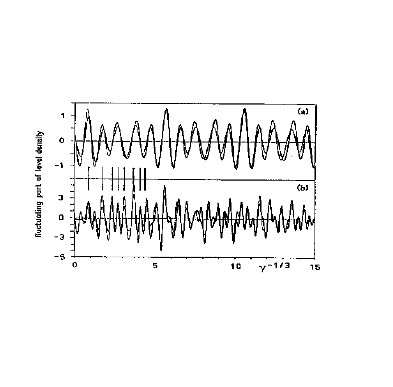
Figure 31: Smoothed fluctuating part of the density of states for the hydrogen atom in a magnetic field at scaled energy $\tilde{E}=-0.2$. The quantum results (thick lines) are smoothed over the first 100 eigenstates. Semiclassical results (thin lines) are obtained by including (a) two orbits (three contributions including repetitions) with scaled actions $s/2\pi<1.33$, and (b) 13 orbits (19 including repetitions) with $s/2\pi<3$. The lowest quantum eigenvalues are marked as vertical bars. (From Ref. [78].)

A first step towards the periodic orbit quantization of mixed systems has been done by Wintgen [78] on the hydrogen atom in a magnetic field. From Gutzwiller’s truncated periodic orbit sum he obtained the smoothed part of the density of states presented in Fig. 31 at scaled energy $\tilde{E}=-0.2$ which is in the mixed regular-chaotic regime. The resolution of the smoothed spectra depends on the cutoff value of the periodic orbit sum which is $s_{\rm max}/2\pi=1.33$ and $s_{\rm max}/2\pi=3.00$ in Fig. 31a and 31b, respectively. Nine approximate eigenvalues have been estimated from the low-resolution truncated periodic orbit sum in Fig. 31b (for comparison the exact quantum eigenvalues are marked by vertical bars in Fig. 31), but neither the accuracy nor the number of semiclassical eigenvalues could be improved by increasing the number of periodic orbits because of the non-convergence property of Gutzwiller’s trace formula. The results of Ref. [78] therefore clearly demonstrate that methods to overcome the convergence problems of the semiclassical periodic orbit sum are of crucial importance to obtain highly resolved semiclassical spectra in the mixed regime. Note also that Gutzwiller’s trace formula is not valid for non-isolated periodic orbits on invariant tori in the regular part of the phase space. This fact has not been considered in Ref. [78].

The limiting cases of mixed systems are strongly chaotic and integrable systems. As has been proven by Gutzwiller [8], for systems with complete chaotic (hyperbolic) classical dynamics the density of states can be expressed as an infinite sum over all (isolated) periodic orbits. On the other extreme of complete integrability, it is well known that the semiclassical energy values can be obtained by EBK torus quantization [1]. This requires the knowledge of all the constants of motion, which are not normally given in explicit form, and therefore practical EBK quantization based on the direct or indirect numerical construction of the constants of motion turns out to be a formidable task [135]. As an alternative, EBK quantization was recast as a sum over all periodic orbits of a given topology on respective tori by Berry and Tabor [25, 26]. The Berry-Tabor formula circumvents the numerical construction of the constants of motion but usually suffers from the convergence problems of the infinite periodic orbit sum.

The extension of the Berry-Tabor formula into the near-integrable (KAM) regime was outlined by Ozorio de Almeida [41] and elaborated, at different levels of refinement, by Tomsovic et al. [27] and Ullmo et al. [28]. These authors noted that in the near-integrable regime, according to the Poincaré-Birkhoff theorem, two periodic orbits survive the destruction of a rational torus with similar actions, one stable and one hyperbolic unstable, and worked out the ensuing modifications of the Berry-Tabor formula. In this section we go one step further by noting that, with increasing perturbation, the stable orbit turns into an inverse hyperbolic one representing, together with its unstable companion with similar action, a remnant torus. We include the contributions of these pairs of inverse hyperbolic and hyperbolic orbits in the Berry-Tabor formula and demonstrate for a system with mixed regular-chaotic dynamics that this procedure yields excellent results even in the deep mixed regular-chaotic regime. As in Ref. [78] we choose the hydrogen atom in a magnetic field, which is a real physical system and has served extensively as a prototype for the investigation of “quantum chaos” [29, 30, 31].

The fundamental obstacle bedeviling the semiclassical quantization of systems with mixed regular-chaotic dynamics is that the periodic orbits are neither sufficiently isolated, as is required for Gutzwiller’s trace formula [8], nor are they part of invariant tori, as is necessary for the Berry-Tabor formula [25, 26]. However, as will become clear below, it is the Berry-Tabor formula which lends itself in a natural way for an extension of periodic orbit quantization to mixed systems. As previously, we consider scaling systems where the classical action $S$ scales as $S=sw$ with $w=\hbar_{\rm eff}^{-1}$ the scaling parameter and $s$ the scaled action. For scaling systems with two degrees of freedom, which we will focus on, the Berry-Tabor formula for the fluctuating part of the level density reads

$$\varrho(w)={1\over\pi}\,{\rm Re}\,\sum_{\bf M}{w^{1/2}s_{\bf M}\over M_{2}^{3/2}|g^{\prime\prime}_{E}|^{1/2}}\,e^{i(s_{\bf M}w-{\pi\over 2}\eta_{\bf M}-{\pi\over 4})}\;,$$ (3.45)

with ${\bf M}=(M_{1},M_{2})$ pairs of integers specifying the individual periodic orbits on the tori (numbers of rotations per period, $M_{2}/M_{1}$ rational), and $s_{\bf M}$ and $\eta_{\bf M}$ the scaled action and Maslov index of the periodic orbit ${\bf M}$. The function $g_{E}$ in (3.45) is obtained by inverting the Hamiltonian, expressed in terms of the actions $(I_{1},I_{2})$ of the corresponding torus, with respect to $I_{2}$, viz. $H(I_{1},I_{2}=g_{E}(I_{1}))=E$ [136]. The calculation of $g^{\prime\prime}_{E}$ from the actions $(I_{1},I_{2})$ can be rather laborious even for integrable and near-integrable systems, and, by definition, becomes impossible for mixed systems in the chaotic part of the phase space. Here we will adopt the method of Refs. [27, 28] and calculate $g^{\prime\prime}_{E}$, for given ${\bf M}=(\mu_{1},\mu_{2})$, with $(\mu_{1},\mu_{2})$ coprime integers specifying the primitive periodic orbit, directly from the parameters of the two periodic orbits (stable (s) and hyperbolic unstable (h)) that survive the destruction of the rational torus $\bf M$, viz.

$$g^{\prime\prime}_{E}={2\over\pi\mu_{2}^{3}\Delta s}\left({1\over\sqrt{\det(M_{\rm s}-I)}}+{1\over\sqrt{-\det(M_{\rm h}-I)}}\right)^{-2}\,,$$ (3.46)

with

$$\Delta s={1\over 2}(s_{\rm h}-s_{\rm s})$$ (3.47)

the difference of the scaled actions, and $M_{\rm s}$ and $M_{\rm h}$ the monodromy matrices of the two orbits. The action $s_{\bf M}$ in (3.45) is to replaced with the mean action

$$\bar{s}={1\over 2}(s_{\rm h}+s_{\rm s})\;.$$ (3.48)

Eq. 3.46 is an approximation which becomes exact in the limit of an integrable system.

It is a characteristic feature of systems with mixed regular-chaotic dynamics that with increasing nonintegrability the stable orbits turn into inverse hyperbolic unstable orbits in the chaotic part of the phase space. These orbits, although embedded in the fully chaotic part of phase space, are remnants of broken tori. It is therefore natural to assume that Eqs. 3.45 and 3.46 can even be applied when these pairs of inverse hyperbolic and hyperbolic orbits are taken into account, i.e., more deeply in the mixed regular-chaotic regime.

It should be noted that the difference $\Delta s$ between the actions of the two orbits is normally still small, and it is therefore more appropriate to start from the Berry-Tabor formula for semiclassical quantization in that regime than from Gutzwiller’s trace formula, which assumes well-isolated periodic orbits. It is also important to note that the Berry-Tabor formula does not require an extensive numerical periodic orbit search. The periodic orbit parameters $s/M_{2}$ and $g^{\prime\prime}_{E}$ are smooth functions of the rotation number $M_{2}/M_{1}$, and can be obtained for arbitrary periodic orbits with coprime integers $(M_{1},M_{2})$ by interpolation between “simple” rational numbers $M_{2}/M_{1}$.

3.4.1 Hydrogen atom in a magnetic field

We now demonstrate the high quality of the extension of Eqs. 3.45 and 3.46 to pairs of inverse hyperbolic and hyperbolic periodic orbits for a physical system that undergoes a transition from regularity to chaos, namely the hydrogen atom in a magnetic field. This is a scaling system, with $w=\gamma^{-1/3}=\hbar_{\rm eff}^{-1}$ the scaling parameter and $\gamma=B/(2.35\times 10^{5}\,{\rm T})$ the magnetic field strength in atomic units. The classical Hamiltonian and the scaling procedure have been discussed in Section 2.1. At low scaled energies $\tilde{E}=E\gamma^{-2/3}<-0.6$ a Poincaré surface of section analysis [30] of the classical Hamiltonian (Eq. 2.11) exhibits two different torus structures related to a “rotator” and “vibrator” type motion. The separatrix between these tori is destroyed at a scaled energy of $\tilde{E}\approx-0.6$, and the chaotic region around the separatrix grows with increasing energy. At $\tilde{E}=-0.127$ the classical phase space becomes completely chaotic. We investigate the system at scaled energy $\tilde{E}=-0.4$, where about 40% of the classical phase space volume is chaotic (see inset in Fig. 32), i.e. well in the region of mixed dynamics. We use 8 pairs of periodic orbits to describe the rotator type motion in both the regular and chaotic region. The results for the periodic orbit parameters $s/2\pi M_{2}$ and $g^{\prime\prime}_{E}$ are presented as solid lines in Fig. 32. The squares on the solid lines mark parameters obtained by pairs of stable and unstable periodic orbits in the regular region of the phase space. The diamonds mark parameters obtained by pairs of two unstable (inverse hyperbolic and hyperbolic) periodic orbits in the chaotic region of phase space. The cutoff is related to the winding angle $\phi=1.278$ of the fixed point of the rotator type motion, i.e., the orbit perpendicular to the magnetic field axis, $(M_{2}/M_{1})_{\rm cutoff}=\pi/\phi=2.458$. The solid lines have been obtained by spline interpolation of the data points. In the same way the periodic orbit parameters for the vibrator type motion have been obtained from 11 pairs of periodic orbits (see the dashed lines in Fig. 32). The cutoff at $M_{2}/M_{1}=\pi/\phi=1.158$ is related to the winding angle $\phi=2.714$ of the fixed point of the vibrator type motion, i.e., the orbit parallel to the field axis.

With the data of Fig. 32 we have all the ingredients at hand to calculate the semiclassical density of states $\varrho(w)$ in Eq. 3.45. The periodic orbit sum includes for both the rotator and vibrator type motion the orbits with $M_{2}/M_{1}>(M_{2}/M_{1})_{\rm cutoff}$. For each orbit the action and the function $g^{\prime\prime}_{E}$ is obtained from the spline interpolations. The Maslov indices are $\eta_{\bf M}=4M_{2}-M_{1}$ for the rotator and $\eta_{\bf M}=4M_{2}+2M_{1}-1$ for the vibrator type orbits. However, the problem is to extract the semiclassical eigenenergies from Eq. 3.45 because the periodic orbit sum does not converge. We now adopt the method discussed in Section 3.2 and adjust the semiclassical recurrence signal, i.e., the Fourier transform of the weighted density of states $w^{-1/2}\varrho(w)$ (Eq. 3.45)

$$C^{\rm sc}(s)=\sum_{\bf M}{\cal A}_{\bf M}\delta(s-s_{\bf M})\;,$$ (3.49)

with the amplitudes being determined exclusively by periodic orbit quantities,

$${\cal A}_{\bf M}={s_{\bf M}\over M_{2}^{3/2}|g^{\prime\prime}_{E}|^{1/2}}\,e^{-i{\pi\over 2}\eta_{\bf M}}\;,$$ (3.50)

to the functional form of its quantum mechanical analogue

$$C^{\rm qm}(s)=-i\sum_{k}d_{k}e^{-iw_{k}s}\;,$$ (3.51)

where the $w_{k}$ are the quantum eigenvalues of the scaling parameter, and the $d_{k}$ are the multiplicities of the eigenvalues ($d_{k}=1$ for nondegenerate states). The frequencies obtained from this procedure are interpreted as the semiclassical eigenvalues $w_{k}$. The technique used to adjust Eq. (3.49) to the functional form of Eq. (3.51) is harmonic inversion [82, 83].

For the hydrogen atom in a magnetic field part of the semiclassical recurrence signal $C^{\rm sc}(s)$ at scaled energy $\tilde{E}=-0.4$ is presented in Fig. 33. The solid and dashed peaks mark the recurrencies of the rotator and vibrator type orbits, respectively. Note that $C^{\rm sc}(s)$ can be easily calculated even for long periods $s$ with the help of the spline interpolation functions in Fig. 32. By contrast, the construction of the recurrence signal for Gutzwiller’s trace formula usually requires an exponentially increasing effort for the numerical periodic orbit search with growing period.

We have analyzed $C^{\rm sc}(s)$ by the harmonic inversion technique in the region $0<s/2\pi<200$. The resulting semiclassical spectrum of the lowest 106 states with eigenvalues $w<20$ is shown in the upper part of Fig. 34a. For graphical purposes the spectrum is presented as a function of the squared scaling parameter $w^{2}$, which is equivalent to unfolding the spectrum to constant mean level spacing. For comparison the lower part of Fig. 34a shows the exact quantum spectrum. The semiclassical and quantum spectrum are seen to be in excellent agreement, and deviations are less than the stick widths for nearly all states. The distribution $P(d)$ of the semiclassical error with $d=(w_{\rm qm}-w_{\rm sc})/\Delta w_{\rm av}$ the error in units of the mean level spacing, $\Delta w_{\rm av}=1.937/w$, is presented in Fig. 34b. For most levels the semiclassical error is less than 4% of the mean level spacing, which is typical for a system with two degrees of freedom [110].

The accuracy of the results presented in Fig. 34 seems to be surprising for two reasons. First, we have not exploited the mean staircase function $\bar{\cal N}(w)$, i.e., the number of eigenvalues $w_{k}$ with $w_{k}<w$, which is a basic requirement of some other semiclassical quantization techniques for bound chaotic systems [65, 61]. Second, as mentioned before, Eq. 3.46 has been derived for near-integrable systems, and is only an approximation, in particular, for mixed systems. We have not taken into account any more refined extensions of the Berry-Tabor formula (3.45) as discussed, e.g., in Refs. [27, 28]. The answer to the second point is that the splitting of scaled actions of the periodic orbit pairs used in Fig. 32 does not exceed $\Delta s=0.022$, and therefore for states with $w<20$ the phase shift between the two periodic orbit contributions is $w\Delta s=0.44$, at most. For small phase shifts the extension of the Berry-Tabor formula to near-integrable systems results in a damping of the amplitudes of the periodic orbit recurrence signal in Fig. 33 but seems not to effect the frequencies, i.e., the semiclassical eigenvalues $w_{k}$ obtained by the harmonic inversion of the function $C^{\rm sc}(s)$.

To summarize, in this section we have presented a solution to the fundamental problem of semiclassical quantization of nonintegrable systems in the mixed regular-chaotic regime. We have demonstrated the excellent quality of our procedure for the hydrogen atom in a magnetic field at a scaled energy $\tilde{E}=-0.4$, where about 40% of the phase space volume is chaotic. The lowest 106 semiclassical and quantum eigenenergies have been shown to agree within a few percent of the mean level spacings. The same method can be applied straightforwardly to other systems with mixed dynamics.

3.5 Harmonic inversion of cross-correlated periodic orbit sums

In the previous sections we have introduced harmonic inversion of semiclassical signals as a powerful and universal technique for the problem of periodic orbit quantization in that it does not depend on special properties of the system such as being bound and ergodic, or the existence of a symbolic dynamics. The method only requires the knowledge of periodic orbits and their physical quantities up to a certain maximum period, which depends on the average local density of states. Unfortunately, this method is not free of the general drawback of most semiclassical approaches, which suffer from a rapid proliferation of periodic orbits with their period, which in turn requires an enormous number of orbits to be taken into account. As discussed in Section 3.1.4 the required signal length for harmonic inversion is at least two times the Heisenberg period. This is by a factor of four longer than the signal length required for the application of the Riemann-Siegel look-alike formula [59, 60, 61]. In chaotic systems, where the number of periodic orbits grows exponentially with the period, the reduction of the required signal length by a factor of four implies that, e.g., instead of one million periodic orbits a reduced set of about 32 orbits is sufficient for the semiclassical quantization. This example clearly illustrates that a shortening of the required signal length is highly desirable.

In this section we want to introduce harmonic inversion of cross-correlated periodic orbit sums as a method to reduce the required amount of periodic orbit data [85]. The idea is that the informational content of a $D\times D$ cross-correlated time signal is increased roughly by a factor of $D$ as compared to a $1\times 1$ signal. The cross-correlated signal is constructed by introducing a set of $D$ smooth and linearly independent operators. Numerically, the harmonic inversion of the cross-correlated periodic orbit sum is based on an extension of the filter-diagonalization method to the case of time cross-correlation functions [68, 137, 138]. This extended method provides highly resolved spectra even in situations of nearly degenerate states, as well as the diagonal matrix elements for the set of operators chosen. The power of the method will be demonstrated in Section 3.7 for the circle billiard, as an example of a completely integrable system.

Consider a quantum Hamiltonian $\hat{H}$ whose eigenvalues are $w_{n}$ and eigenstates $|n\rangle$. [As previously, we consider scaling systems with $w$ the scaling parameter, which is not necessarily the energy, and with linear scaling of the classical action, $S_{\rm po}=ws_{\rm po}$.] We introduce a cross-correlated response function $(\alpha,\beta=1,2,\dots,D)$

$$g_{\alpha\beta}(w)=\sum_{n}{b_{\alpha n}b_{\beta n}\over w-w_{n}+i0}\ ,$$ (3.52)

where $b_{\alpha n}$ and $b_{\beta n}$ are the diagonal matrix elements of two operators $\hat{A}_{\alpha}$ and $\hat{A}_{\beta}$, respectively, i.e.

$$b_{\alpha n}=\langle n|\hat{A}_{\alpha}|n\rangle\;.$$ (3.53)

Later we have to find a semiclassical approximation to Eq. 3.52. In this context it is important to note that $g_{\alpha\beta}(w)$ can only be written as a trace formula,

$$g_{\alpha\beta}(w)=\mbox{tr}\,\left\{\hat{A}_{\alpha}\hat{G}^{+}(w)\hat{A}_{\beta}\right\}$$

with the Green Function

$$\hat{G}^{+}(w)={1\over w-\hat{H}+i0}\;,$$

if either $\hat{A}_{\alpha}$ or $\hat{A}_{\beta}$ commutes with $\hat{H}$. The weighted density of states is given by

$$\varrho_{\alpha\beta}(w)=-{1\over\pi}\,{\rm Im}\,g_{\alpha\beta}(w)\ .$$ (3.54)

Let us assume that the semiclassical approximation $g_{\alpha\beta}^{\rm sc}(w)$ to the quantum expression (3.52) is given. The general procedure of harmonic inversion as described in Section 3.2 would then be to adjust the Fourier transform of $g_{\alpha\beta}^{\rm sc}(w)$ to the functional form of the quantum expression

$$C_{\alpha\beta}^{\rm qm}(s)={1\over 2\pi}\int_{-\infty}^{+\infty}g_{\alpha\beta}^{\rm qm}(w)e^{-isw}dw=-i\sum_{n}b_{\alpha n}b_{\beta n}e^{-iw_{n}s}\;.$$ (3.55)

The conventional harmonic inversion problem is formulated as a nonlinear fit of the signal $C(s)$ by the sum of sinusoidal terms (see Section 2.2 and Appendix A.1),

$$C(s)=\sum_{n}d_{n}e^{-iw_{n}s}\;,$$

with the set of, in general, complex variational parameters $\{w_{n},d_{n}=-ib_{\alpha n}b_{\beta n}\}$. As already discussed in Section 3.1.4, simple information theoretical considerations then yield an estimate for the required signal length, $s_{\rm max}\sim 4\pi\bar{\varrho}(w)$, for poles $w_{n}\leq w$ which can be extracted by this method. When a periodic orbit approximation of the quantum signal $C(s)$ is used, this estimate results sometimes in a very unfavorable scaling because of a rapid (exponential for chaotic systems) proliferation of periodic orbits with increasing period. Let us consider now a generalized harmonic inversion problem, which assumes that the whole $s$-dependent $D\times D$ signal $C_{\alpha\beta}(s)$ is adjusted simultaneously to the form of Eq. 3.55, with $b_{\alpha n}$ and $w_{n}$ being the variational parameters. The advantage of using the cross-correlation approach [68, 137, 138] is based on the simple argument that the total amount of independent information contained in the $D\times D$ signal is $D(D+1)$ multiplied by the length of the signal, while the total number of unknowns (here $b_{\alpha n}$ and $w_{n}$) is $(D+1)$ times the total number of poles $w_{n}$. Therefore the informational content of the $D\times D$ signal per unknown parameter is increased (compared to the case of Eq. 3.32) by a factor of $D$. [Of course, this scaling holds only approximately and for sufficiently small numbers $D$ of operators $\hat{A}_{\alpha}$ chosen.] Thus we have the result that, provided we are able to obtain a periodic orbit approximation for $C_{\alpha\beta}(s)$, with this procedure we can extract more information from the same set of periodic orbits.

We now have to find a semiclassical approximation for $C_{\alpha\beta}(s)$ in Eq. 3.55. The problem has been solved in the literature only for special cases, i.e., if one or both operators $\hat{A}_{\alpha}$ and $\hat{A}_{\beta}$ are the identity or, somewhat more general, if at least one of the operators commutes with the Hamiltonian $\hat{H}$. For the identity operator $\hat{A}_{1}=I$ the element $C_{11}^{\rm sc}(s)$ is the Fourier transform of Gutzwiller’s trace formula [7, 8] for chaotic systems, and of the Berry-Tabor formula [25, 26] for regular systems, i.e.

$$C_{11}^{\rm sc}(s)=\sum_{\rm po}{\cal A}_{\rm po}\delta\left(s-s_{\rm po}\right)\;,$$ (3.56)

where $s_{\rm po}$ are the periods of the orbits and ${\cal A}_{\rm po}$ the amplitudes (recurrence strengths) of the periodic orbit contributions including phase information. For $\hat{A}_{1}=I$ and an arbitrary smooth operator $\hat{A}_{\alpha}$ the elements $C_{\alpha 1}^{\rm sc}(s)$ are obtained from a semiclassical approximation to the generalized trace formula

$$g_{\alpha 1}(w)={\rm tr}\,\left\{\hat{G}^{+}(w)\hat{A}_{\alpha}\right\}\;,$$ (3.57)

which has been investigated in detail in Refs. [128, 129]. The result is that the amplitudes ${\cal A}_{\rm po}$ in (3.56) have to be multiplied by the classical average of the observable $A_{\alpha}$ along the periodic orbit,

$$a_{\alpha,{\rm po}}={1\over s_{\rm po}}\int_{0}^{s_{\rm po}}A_{\alpha}({\bf q}(s),{\bf p}(s))ds\;,$$ (3.58)

with $A_{\alpha}({\bf q},{\bf p})$ the Wigner transform of the operator $\hat{A}_{\alpha}$, i.e., the signal $C_{\alpha 1}^{\rm sc}(s)$ reads

$$C_{\alpha 1}^{\rm sc}(s)=\sum_{\rm po}a_{\alpha,{\rm po}}{\cal A}_{\rm po}\delta\left(s-s_{\rm po}\right)\;.$$ (3.59)

If at least one of the operators $\hat{A}_{\alpha}$ and $\hat{A}_{\beta}$ commutes with $\hat{H}$, Eq. 3.52 can still be written as a trace formula,

$$g_{\alpha\beta}(w)={\rm tr}\,\left\{\hat{A}_{\alpha}\hat{G}^{+}(w)\hat{A}_{\beta}\right\}={\rm tr}\,\left\{\hat{G}^{+}(w)\left(\hat{A}_{\alpha}\hat{A}_{\beta}\right)\right\}\;,$$

and Eq. 3.59 can be applied to the product $\hat{A}_{\alpha}\hat{A}_{\beta}$. However, we do not want to restrict the operators to those commuting with $\hat{H}$, which obviously would be a severe restriction especially for chaotic systems, and the problem is now to find a semiclassical approximation to Eq. 3.55 for the general case of two arbitrary smooth operators $\hat{A}_{\alpha}$ and $\hat{A}_{\beta}$. A reasonable assumption is that the amplitudes ${\cal A}_{\rm po}$ in (3.56) have to be multiplied by the product of the classical averages, $a_{\alpha,{\rm po}}a_{\beta,{\rm po}}$, of these two observables, i.e.

$$C_{\alpha\beta}^{\rm sc}(s)=\sum_{\rm po}a_{\alpha,{\rm po}}a_{\beta,{\rm po}}{\cal A}_{\rm po}\delta\left(s-s_{\rm po}\right)\;.$$ (3.60)

Although no rigorous mathematical proof of Eq. 3.60 will be given here, we have strong numerical evidence, from the high resolution analysis of quantum spectra, part of which will be given below, that the conjecture of Eq. 3.60 is correct. Details on semiclassical non-trace type formulae like Eq. 3.60 are given in Ref. [139]. Eq. 3.60 is the starting point for the following application of harmonic inversion of cross-correlation functions. Note that all quantities in (3.60) are obtained from the classical periodic orbits.

The idea of periodic orbit quantization by harmonic inversion of cross-correlated periodic orbit sums is to fit the semiclassical functions $C_{\alpha\beta}^{\rm sc}(s)$ given in a finite range $0<s<s_{\rm max}$ to the functional form of the quantum expression (3.55). As for the harmonic inversion of a one-dimensional signal (see Section 3.2) the frequencies of the harmonic inversion analysis are then identified with the semiclassical eigenvalues $w_{n}$. The amplitudes $b_{\alpha n}$ are identified with the semiclassical approximations to the diagonal matrix elements $\langle n|\hat{A}_{\alpha}|n\rangle$. Here we only give a brief description how the harmonic inversion method is extended to cross-correlation functions. The details of the numerical procedure of solving the generalized harmonic inversion problem (3.55) are presented in Refs. [68, 137, 138] and in Appendix A.2. As for the harmonic inversion of a single function the idea is to recast the nonlinear fit problem as a linear algebraic problem [68]. This is done by associating the signal $C_{\alpha\beta}(s)$ (to be inverted) with a time cross-correlation function between an initial state $\Phi_{\alpha}$ and a final state $\Phi_{\beta}$,

$$C_{\alpha\beta}(s)=\left(\Phi_{\beta},e^{-i\hat{\Omega}s}\Phi_{\alpha}\right)\;,$$ (3.61)

where the fictitious quantum dynamical system is described by an effective Hamiltonian $\hat{\Omega}$. The latter is defined implicitly by relating its spectrum to the set of unknown spectral parameters $w_{n}$ and $b_{\alpha n}$. Diagonalization of $\hat{\Omega}$ would yield the desired $w_{n}$ and $b_{\alpha n}$. This is done by introducing an appropriate basis set in which the matrix elements of $\hat{\Omega}$ are available only in terms of the known signals $C_{\alpha\beta}(s)$. The Hamiltonian $\hat{\Omega}$ is assumed to be complex symmetric even in the case of a bound system. This makes the harmonic inversion stable with respect to “noise” due to the imperfections of the semiclassical approximation. The most efficient numerical and practical implementation of the harmonic inversion method with all relevant formulae can be found in Refs. [137, 138] and Appendix A.2.

The method of harmonic inversion of cross-correlated periodic orbit sums will be applied in Section 3.7 to the circle billiard. As will be shown, for a given number of periodic orbits the accuracy of semiclassical spectra can be significantly improved with the help of the cross-correlation approach, or, alternatively, spectra with similar accuracy can be obtained from a periodic orbit cross-correlation signal with significantly reduced signal length.

3.6 $\hbar$ expansion for the periodic orbit quantization by harmonic inversion

Semiclassical spectra can be obtained for both regular and chaotic systems in terms of the periodic orbits of the system. For chaotic dynamics the semiclassical trace formula was derived by Gutzwiller [7, 8], and for integrable systems the Berry-Tabor formula [25, 26] is well known to be precisely equivalent to the EBK torus quantization [1, 2, 3]. However, as already has been discussed in Section 2.6, the semiclassical trace formulae are exact only in exceptional cases, e.g., the geodesic motion on the constant negative curvature surface. In general, they are just the leading order terms of an infinite series in powers of the Planck constant and the accuracy of semiclassical quantization is still an object of intense investigation [109, 110, 140]. Methods for the calculation of the higher order periodic orbit contributions were developed in Refs. [22, 23, 24]. In Section 2.6 we have demonstrated how the periodic orbit quantities of the $\hbar$ expanded trace formula can be extracted from the quantum and semiclassical spectra. It is an even more fundamental problem to obtain semiclassical eigenenergies beyond the Gutzwiller and Berry-Tabor approximation directly from the $\hbar$ expanded periodic orbit sum. Note that the $\hbar$ expansion of the periodic orbit sum does not solve the general problem of the construction of the analytic continuation of the trace formula, which is already a fundamental problem when only the leading order terms of the $\hbar$ expansion is considered. Up to now the $\hbar$ expansion for periodic orbit quantization is restricted to systems with known symbolic dynamics, like the three disk scattering problem, where cycle expansion techniques can be applied [23, 24], and semiclassical eigenenergies beyond the Gutzwiller and Berry-Tabor approximation cannot be calculated, e.g., for bound systems with the help of Riemann-Siegel type formulae [60, 61] or surface of section techniques [62, 63]. In this section we extend the method of periodic orbit quantization by harmonic inversion to the analysis of the $\hbar$ expansion of the periodic orbit sum. The accuracy of semiclassical eigenvalues can be improved by one to several orders of magnitude, as will be shown in Section 3.7 by way of example of the circle billiard.

As in Section 2.6 we consider systems with a scaling property, i.e., where the classical action scales as $S_{\rm po}=ws_{\rm po}$, and the scaling parameter $w\equiv\hbar_{\rm eff}^{-1}$ plays the role of an inverse effective Planck constant. The $\hbar$ expansion of the periodic orbit sum is given (see Eq. 2.65) as a power series in $w^{-1}$,

$$g(w)=\sum_{n=0}^{\infty}g_{n}(w)=\sum_{n=0}^{\infty}{1\over w^{n}}\sum_{\rm po}{\cal A}_{\rm po}^{(n)}e^{is_{\rm po}w}\;.$$ (3.62)

The complex amplitudes ${\cal A}_{\rm po}^{(n)}$ of the $n^{\rm th}$ order periodic orbit contributions include the phase information from the Maslov indices. For periodic orbit quantization the zeroth order contributions ${\cal A}_{\rm po}^{(0)}$ are usually considered only. The Fourier transform of the principal periodic orbit sum

$$C_{0}(s)={1\over 2\pi}\int_{-\infty}^{+\infty}g_{0}(w)e^{-isw}dw=\sum_{\rm po}{\cal A}_{\rm po}^{(0)}\delta(s-s_{\rm po})$$ (3.63)

is adjusted by application of the harmonic inversion technique (see Section 3.2) to the functional form of the exact quantum expression

$$C(s)={1\over 2\pi}\int_{-\infty}^{+\infty}\sum_{k}{d_{k}\over w-w_{k}+i0}e^{-iws}dw=-i\sum_{k}d_{k}e^{-iw_{k}s}\;,$$ (3.64)

with $\{w_{k},d_{k}\}$ the eigenvalues and multiplicities. The frequencies $w_{k,0}$ obtained by harmonic inversion of Eq. 3.63 are the zeroth order $\hbar$ approximation to the semiclassical eigenvalues. We will now demonstrate how the higher order correction terms to the semiclassical eigenvalues can be extracted from the periodic orbit sum (3.62). We first remark that the asymptotic expansion (3.62) of the semiclassical response function suffers, for $n\geq 1$, from the singularities at $w=0$, and it is therefore not appropriate to harmonically invert the Fourier transform of (3.62), although the Fourier transform formally exists. This means that the method of periodic orbit quantization by harmonic inversion cannot straightforwardly be extended to the $\hbar$ expansion of the periodic orbit sum. Instead we will calculate the correction terms to the semiclassical eigenvalues separately, order by order, as described in the following.

Let us assume that the $(n-1)^{\rm st}$ order approximations $w_{k,n-1}$ to the semiclassical eigenvalues are already obtained and the $w_{k,n}$ are to be calculated. The difference between the two subsequent approximations to the quantum mechanical response function reads [86]

$$g_{n}(w) = \sum_{k}\left({d_{k}\over w-w_{k,n}+i0}-{d_{k}\over w-w_{k,n-1}+i0}\right)$$ (3.65)

$$\approx \sum_{k}{d_{k}\Delta w_{k,n}\over(w-\bar{w}_{k,n}+i0)^{2}}\;,$$

with $\bar{w}_{k,n}=(w_{k,n}+w_{k,n-1})/2$ and $\Delta w_{k,n}=w_{k,n}-w_{k,n-1}$. Integration of Eq. 3.65 and multiplication by $w^{n}$ yields

$${\cal G}_{n}(w)=w^{n}\int g_{n}(w)dw=\sum_{k}{-d_{k}w^{n}\Delta w_{k,n}\over w-\bar{w}_{k,n}+i0}\;,$$ (3.66)

which has the functional form of a quantum mechanical response function but with residues proportional to the $n^{\rm th}$ order corrections $\Delta w_{k,n}$ to the semiclassical eigenvalues. The semiclassical approximation to Eq. 3.66 is obtained from the term $g_{n}(w)$ in the periodic orbit sum (3.62) by integration and multiplication by $w^{n}$, i.e.

$${\cal G}_{n}(w)=w^{n}\int g_{n}(w)dw=-i\sum_{\rm po}{1\over s_{\rm po}}{\cal A}_{\rm po}^{(n)}e^{iws_{\rm po}}+{\cal O}\left(1\over w\right)\;.$$ (3.67)

We can now Fourier transform both Eqs. 3.66 and 3.67, and obtain ($n\geq 1$)

$$C_{n}(s) \equiv {1\over 2\pi}\int_{-\infty}^{+\infty}{\cal G}_{n}(w)e^{-iws}dw=i\sum_{k}d_{k}(w_{k})^{n}\Delta w_{k,n}e^{-iw_{k}s}$$ (3.68)

$$\stackrel{{\scriptstyle\rm h.i.}}{{=}} -i\sum_{\rm po}{1\over s_{\rm po}}{\cal A}_{\rm po}^{(n)}\delta(s-s_{\rm po})\;.$$ (3.69)

Eqs. 3.68 and 3.69 are the main result of this section. They imply that the $\hbar$ expansion of the semiclassical eigenvalues can be obtained, order by order, by harmonic inversion (h.i.) of the periodic orbit signal in Eq. 3.69 to the functional form of Eq. 3.68. The frequencies of the periodic orbit signal (3.69) are the semiclassical eigenvalues $w_{k}$. Note that the accuracy of the semiclassical eigenvalues does not necessarily increase with increasing order $n$. We indicate this in Eq. 3.68 by omitting the index $n$ at the eigenvalues $w_{k}$. The corrections $\Delta w_{k,n}$ to the eigenvalues are obtained from the amplitudes, $d_{k}(w_{k})^{n}\Delta w_{k,n}$, of the periodic orbit signal.

The method requires as input the periodic orbits of the classical system up to a maximum period (scaled action), $s_{\rm max}$, determined by the average density of states [82, 83]. The amplitudes ${\cal A}_{\rm po}^{(0)}$ are obtained from Gutzwiller’s trace formula [7, 8] and the Berry-Tabor formula [25, 26] for chaotic and regular systems, respectively. For the next order correction ${\cal A}_{\rm po}^{(1)}$ explicit formulae were derived by Gaspard and Alonso for chaotic systems with smooth potentials [22] and in Refs. [23, 24] for billiards. With appropriate modifications [87, 88] the formulae can be used for regular systems as well. As an example we investigate the $\hbar$ expansion of the periodic orbit sum for the circle billiard in the next section.

3.7 The circle billiard

In Section 3.5 (see also [85]) we have introduced harmonic inversion of cross-correlated periodic orbit sums as a method to significantly reduce the required number of periodic orbits for semiclassical quantization, and in Section 3.6 (see also [86]) we have discussed the $\hbar$ expansion of the periodic orbit sum and the calculation of semiclassical eigenenergies beyond the Gutzwiller [8] and Berry-Tabor [25, 26] approximation. We now demonstrate both methods by way of example of the circle billiard. The circle billiard is a regular system and has been chosen here for the following reasons.

1. The nearest neighbor level statistics of integrable systems is a Poisson distribution, with a high probability for nearly degenerate states. The conventional method for periodic orbit quantization by harmonic inversion requires very long signals to resolve the nearly degenerate states. We will demonstrate the power of harmonic inversion of cross-correlated periodic orbit sums by fully resolving those nearly degenerate states with a significantly reduced set of orbits.

2. All relevant physical quantities, i.e., the quantum and semiclassical eigenenergies, the matrix elements of operators, the periodic orbits and their zeroth and first order amplitudes of the $\hbar$ expanded periodic orbit sum, and the periodic orbit averages of classical observables can easily be obtained.

3. The semiclassical quantization of the circle billiard as an example of an integrable system demonstrates the universality and wide applicability of periodic orbit quantization by harmonic inversion, i.e., the method is not restricted to systems with hyperbolic dynamics like, e.g., pinball scattering.

The circle billiard has already been introduced in Section 2.6.1. The exact quantum mechanical eigenvalues $E=\hbar^{2}k^{2}/2M$ are given as zeros of Bessel functions $J_{|m|}(kR)=0$, where $m$ is the angular momentum quantum number and $R$, the radius of the circle. In the following we choose $R=1$. The semiclassical eigenvalues are obtained from the EBK quantization condition, Eq. 2.71,

$$kR\sqrt{1-(m/kR)^{2}}-|m|\arccos{|m|\over kR}=\pi\left(n+{3\over 4}\right)\;,$$

and the $\hbar$ expansion of the periodic orbit sum reads (see Eq. 2.73)

$${1\over\sqrt{k}}g(k)={1\over\sqrt{k}}\sum_{n=0}^{\infty}g_{n}(k)=\sum_{n=0}^{\infty}{1\over k^{n}}\sum_{\rm po}{\cal A}_{\rm po}^{(n)}e^{i\ell_{\rm po}k}\;,$$

with (see Eqs. 2.74 and 2.75)

$${\cal A}_{\rm po}^{(0)} = \sqrt{\pi\over 2}{\ell_{\rm po}^{3/2}\over m_{r}^{2}}\,e^{-i({\pi\over 2}\mu_{\rm po}+{\pi\over 4})}\;,$$

$${\cal A}_{\rm po}^{(1)} = {1\over 2}\sqrt{\pi m_{r}}\,{5-2\sin^{2}\gamma\over 3\sin^{3/2}\gamma}\,e^{-i({\pi\over 2}\mu_{\rm po}-{\pi\over 4})}\;.$$

The angle $\gamma$ is defined as $\gamma\equiv\pi m_{\phi}/m_{r}$, with $m_{\phi}=1,2,\dots$ the number of turns of the periodic orbit around the origin, and $m_{r}=2m_{\phi},2m_{\phi}+1,\dots$ the number of reflections at the boundary of the circle. $\ell_{\rm po}=2m_{r}\sin\gamma$ and $\mu_{\rm po}=3m_{r}$ are the geometrical length and Maslov index of the orbits, respectively.

3.7.1 Harmonic inversion of the cross-correlated periodic orbit sum

We now calculate the semiclassical eigenenergies of the circle billiard by harmonic inversion of the cross-correlated periodic orbit sum (3.60) with ${\cal A}_{\rm po}={\cal A}_{\rm po}^{(0)}$ (Eq. 2.74) the amplitudes of the Berry-Tabor formula [25, 26], i.e., the lowest order $\hbar$ approximation. To construct the periodic orbit cross-correlation signal $C_{\alpha\beta}^{\rm sc}(\ell)$ we choose three different operators,

$$\hat{A}_{1}=I$$

the identity,

$$\hat{A}_{2}=r$$

the distance from the origin, and

$$\hat{A}_{3}=(L/k)^{2}$$

the square of the scaled angular momentum. For these operators the classical weights $a_{\alpha,{\rm po}}$ (Eq. 3.58) are obtained as

$$a_{1,{\rm po}} = 1$$

$$a_{2,{\rm po}} = {1\over 2}\left(1+{\cos\gamma\over\tan\gamma}{\rm arsinh}\,\tan\gamma\right)$$ (3.70)

$$a_{3,{\rm po}} = \cos^{2}\gamma\;.$$

Once all the ingredients of Eq. 3.60 for the circle billiard are available, the $3\times 3$ periodic orbit cross-correlation signal $C_{\alpha\beta}^{\rm sc}(\ell)$ can easily be constructed and inverted by the generalized filter-diagonalization method. Results obtained from the periodic orbits with maximum length $s_{\rm max}=100$ are presented in Fig. 35. Fig. 35a is part of the density of states, $\varrho(k)$, Figs. 35b and 35c are the density of states weighted with the diagonal matrix elements of the operators $\hat{A}=r$ and $\hat{A}=L^{2}$, respectively. The squares are the results from the harmonic inversion of the periodic orbit cross-correlation signals. For comparison the crosses mark the matrix elements obtained by exact quantum calculations at positions $k^{\rm EBK}$ obtained from the EBK quantization condition (2.71). In this section we do not compare with the exact zeros of the Bessel functions because Eq. 3.60 is correct only to first order in $\hbar$ and thus the harmonic inversion of $C_{\alpha\beta}^{\rm sc}(s)$ cannot provide the exact quantum mechanical eigenvalues. The calculation of eigenenergies beyond the Berry-Tabor approximation will be discussed in Section 3.7.2. However, the perfect agreement between the eigenvalues $k^{\rm HI}$ obtained by harmonic inversion and the EBK eigenvalues $k^{\rm EBK}$ is remarkable, and this is even true for nearly degenerate states marked by arrows in Fig. 35a. The eigenvalues of some nearly degenerate states are presented in Table 11. It is important to emphasize that these states with level splittings of, e.g., $\Delta k=6\times 10^{-4}$ cannot be resolved by the originally proposed method of periodic orbit quantization by harmonic inversion (see Section 3.2) with a periodic orbit signal length $s_{\rm max}=100$. To resolve the two levels at $k\approx 11.049$ (see Table 11) a signal length of at least $s_{\rm max}\approx 500$ is required if a single periodic orbit function $C^{\rm sc}(s)$ is used instead of a cross-correlation function. The method presented in Section 3.5 can therefore be used to significantly reduce the required signal length and thus the required number of periodic orbits for periodic orbit quantization by harmonic inversion. As such the part of the spectrum shown in Fig. 35 can even be resolved, apart from the splittings of the nearly degenerate states marked by the arrows, from a short cross-correlation signal with $s_{\rm max}=30$, which is about the Heisenberg period $s_{H}=2\pi\bar{\varrho}(k)$, i.e. half of the signal length required for the harmonic inversion of a $1\times 1$ signal. With five operators and a $5\times 5$ cross-correlation signal highly excited states around $k=130$ have even been obtained with a signal length $s_{\rm max}\approx 0.7s_{H}$ [87, 88], which is close to the signal length $s_{\rm max}\approx 0.5s_{H}$ required for the Riemann-Siegel type quantization [59, 60, 61]. The reduction of the signal length is especially important if the periodic orbit parameters are not given analytically, as in our example of the circle billiard, but must be obtained from a numerical periodic orbit search. How small can $s_{\rm max}$ get as one uses more and more operators in the method? It might be that half of the Heisenberg period is a fundamental barrier for bound systems with chaotic dynamics in analogy to the Riemann-Siegel formula [61] while for regular systems an even further reduction of the signal length should in principle be possible. However, further investigations are necessary to clarify this point.

3.7.2 Periodic orbit quantization beyond the Berry-Tabor approximation

The semiclassical eigenvalues obtained by harmonic inversion of a cross-correlated or a sufficiently long single signal are in excellent agreement with the results of the EBK torus quantization, Eq. 2.71. However, they deviate from the exact quantum mechanical eigenenergies, i.e., the zeros of the Bessel functions because the Berry-Tabor formula [25, 26] is only the lowest order $\hbar$ approximation of the periodic orbit sum. We now demonstrate the $\hbar$ expansion of the periodic orbit sum and apply the technique discussed in Section 3.6 to the circle billiard.

The first order corrections to the semiclassical eigenvalues, $\Delta k=k^{(1)}-k^{(0)}$ are obtained by harmonic inversion of the periodic orbit signal $C_{1}(\ell)$ (see Eq. 3.69),

$$C_{1}(\ell)=-i\sum_{\rm po}{1\over\ell_{\rm po}}{\cal A}_{\rm po}^{(1)}\delta(\ell-\ell_{\rm po})\stackrel{{\scriptstyle\rm h.i.}}{{=}}i\sum_{j}d_{j}k_{j}^{(0)}\left[k_{j}^{(1)}-k_{j}^{(0)}\right]\,e^{-ik_{j}\ell}\;,$$ (3.71)

with $d_{j}$ the multiplicities of states. The signal $C_{1}(\ell)$ in Eq. 3.71 can be inverted as a single function as has been done in Ref. [86], where the accuracy of the eigenenergies was improved by one to several orders of magnitude, apart from the nearly degenerate states marked by arrows in Fig. 35. Here we go one step further and use Eq. 3.71 as part of a $3\times 3$ cross-correlation signal. For the two other diagonal components of the cross-correlation matrix we use the identity operator, $\hat{A}_{1}=I$, and the distance from the origin, $\hat{A}_{2}=r$. By applying the cross-correlation technique of Section 3.5 we obtain both the zeroth and first order $\hbar$ expansion of the eigenenergies and the diagonal matrix elements of the chosen operators simultaneously from one and the same harmonic inversion procedure. Furthermore, we can now even resolve the nearly degenerate states. The spectrum of the integrated differences of the density of states $\int\Delta\varrho(k)dk$ obtained by harmonic inversion of the $3\times 3$ cross-correlation matrix with signal length $\ell_{\rm max}=150$ is shown in Fig. 36. The squares mark the spectrum for $\Delta\varrho(k)=\varrho^{\rm(1)}(k)-\varrho^{\rm(0)}(k)$ obtained from the harmonic inversion of the signal $C_{1}(s)$. For comparison the crosses present the same spectrum but for the difference $\Delta\varrho(k)=\varrho^{\rm ex}(k)-\varrho^{\rm EBK}(k)$ between the exact quantum mechanical and the EBK-spectrum. The deviations between the peak heights exhibit the contributions of terms of the $\hbar$ expansion series beyond the first order approximation. The peak heights of the levels in Fig. 36 (solid lines and crosses) are, up to a multiplicity factor for the degenerate states, the shifts $\Delta k$ between the zeroth and first order semiclassical approximations to the eigenvalues $k$. The zeroth and first order eigenvalues, $k^{(0)}$ and $k^{(1)}=k^{(0)}+\Delta k$ are presented in Table 12 for the 40 lowest eigenstates. The zeroth order eigenvalues, $k^{(0)}$, agree within the numerical accuracy with the results of the torus quantization, Eq. 2.71 (see eigenvalues $k^{\rm EBK}$ in Table 12). However, the semiclassical eigenvalues deviate significantly, especially for states with low radial quantum numbers $n$, from the exact quantum mechanical eigenvalues $k^{\rm ex}$ in Table 12. By contrast, the semiclassical error of the first order eigenvalues, $k^{(1)}$, is by orders of magnitude reduced compared to the lowest order approximation.

An appropriate measure for the accuracy of semiclassical eigenvalues is the deviation from the exact quantum eigenvalues in units of the average level spacings, $\langle\Delta k\rangle_{\rm av}=1/\bar{\varrho}(k)$. Fig. 37 presents the semiclassical error in units of the average level spacings $\langle\Delta k\rangle_{\rm av}\approx 4/k$ for the zeroth order (diamonds) and first order (crosses) approximations to the eigenvalues. In the zeroth order approximation the semiclassical error for the low lying states is about 3 to 10 percent of the mean level spacing. This error is reduced in the first order approximation by at least one order of magnitude for the least semiclassical states with radial quantum number $n=0$. The accuracy of states with $n\geq 1$ is improved by two or more orders of magnitude.

Finally, we want to note that the small splittings between the nearly degenerate states are extremely sensitive to the higher order $\hbar$ corrections. E.g., in the zeroth order approximation the splitting between the two states around $k\approx 11.05$ is $\Delta k^{(0)}=6\times 10^{-4}$. In the first order approximation the splitting between the same states is $\Delta k^{(1)}=0.0242$, which is very close to the exact splitting $\Delta k^{\rm ex}=0.0217$. The accuracy obtained here for the first order approximations to the nearly degenerate states goes beyond the results presented in Ref. [86], and is achieved by the combined application of the methods introduced in Sections 3.5 and 3.6, i.e., the harmonic inversion of cross-correlation functions and the analysis of the $\hbar$ expanded periodic orbit sum, respectively.

3.8 Semiclassical calculation of transition matrix elements for atoms in external fields

The interpretation of photoabsorption spectra of atoms in external fields is a fundamental problem of atomic physics. Although the “exact” quantum mechanics accurately describes the energies and transition strengths of individual levels it has completely failed to present a simple physical picture of the long ranged modulations which have been observed in early low resolution spectra of barium atoms in a magnetic field [141] and later in the Fourier transform recurrence spectra of the magnetized hydrogen atom [142, 71]. However, the long ranged modulations of the quantum photoabsorption spectra can be naturally interpreted in terms of the periods of classical closed orbits starting at and returning back to the nucleus where the initial state is localized. The link between the quantum spectra and classical trajectories is given by closed orbit theory [90, 91, 92, 93] which describes the photoabsorption cross section as the sum of a smooth part and the superposition of sinusoidal modulations. The frequencies, amplitudes, and phases of the modulations are directly obtained from the quantities of the closed orbits. When the photoabsorption spectra are Fourier transformed or analyzed with a high resolution method (see Sections 2.1 to 2.3) the sinusoidal modulations result in sharp peaks in the Fourier transform recurrence spectra, and closed orbit theory has been most successful to explain quantum mechanical recurrence spectra qualitatively and even quantitatively in terms of the closed orbits of the underlying classical system [46, 47, 48, 51].

However, up to now practical applications of closed orbit theory have always been restricted to the semiclassical calculation of low resolution photoabsorption spectra for the following two reasons. First, the closed orbit sum requires, in principle, the knowledge of all orbits up to infinite length, which are usually not available from a numerical closed orbit search, and second, the infinite closed orbit sum suffers from fundamental convergence problems [90, 91, 92, 93]. It is therefore commonly accepted that the calculation of individual transition matrix elements $\langle\phi_{i}|D|\psi_{f}\rangle$ of the dipole operator $D$, which describe the transition strengths from the initial state $|\phi_{i}\rangle$ to final states $|\psi_{f}\rangle$, is a problem beyond the applicability of the semiclassical closed orbit theory, i.e., is the domain of quantum mechanical methods.

In this section we disprove this common believe and demonstrate that individual eigenenergies and transition matrix elements can be directly extracted from the quantities of the classical closed orbits. To that end, we slightly generalize closed orbit theory to the semiclassical calculation of cross-correlated recurrence functions. We then adopt the cross-correlation approach introduced in Section 3.5 to harmonically invert the cross-correlated recurrence signal and to extract the semiclassical eigenenergies and transition matrix elements. Results will be presented for the photo excitation of the hydrogen atom in a magnetic field.

The oscillator strength $f$ for the photo excitation of atoms in external fields can be written as

$$f(E)=-{2\over\pi}(E-E_{i})\>{\rm Im}\,\langle\phi_{i}|DG_{E}^{+}D|\phi_{i}\rangle\;,$$ (3.72)

where $|\phi_{i}\rangle$ is the initial state at energy $E_{i}$, $D$ is the dipole operator, and $G_{E}^{+}$ the retarded Green’s function of the atomic system. The basic steps for the derivation of closed orbit theory are to replace the quantum mechanical Green’s function in (3.72) with its semiclassical Van Vleck-Gutzwiller approximation and to carry out the overlap integrals with the initial state $|\phi_{i}\rangle$. Here we go one step further by introducing a cross-correlation matrix

$$g_{\alpha\alpha^{\prime}}=\langle\phi_{\alpha}|DG_{E}^{+}D|\phi_{\alpha^{\prime}}\rangle$$ (3.73)

with $|\phi_{\alpha}\rangle$, $\alpha=1,2,\dots,L$ a set of independent initial states. As will be shown below the use of cross-correlation matrices can considerably improve the convergence properties of the semiclassical procedure. In the following we will concentrate on the hydrogen atom in a magnetic field with $\gamma=B/(2.35\times 10^{5}\,{\rm T})$ the magnetic field strength in atomic units. As discussed in Section 2.1 the system has a scaling property, i.e., the shape of periodic orbits does not depend on the scaling parameter, $w=\gamma^{-1/3}=\hbar_{\rm eff}^{-1}$, and the classical action scales as $S=sw$ with $s$ the scaled action. As, e.g., in Ref. [47] we consider scaled photoabsorption spectra at constant scaled energy $\tilde{E}=E\gamma^{-2/3}$ as a function of the scaling parameter $w$. We choose dipole transitions between states with magnetic quantum number $m=0$. Note that the following ideas can be applied in an analogous way to atoms in electric fields. Following the derivation of Refs. [91, 93] the semiclassical approximation to the fluctuating part of $g_{\alpha\alpha^{\prime}}$ in Eq. 3.73 reads

$$g_{\alpha\alpha^{\prime}}^{\rm sc}(w) = w^{-1/2}\sum_{{\rm co}}{-(2\pi)^{5/2}\over\sqrt{|m_{12}^{\rm co}|}}\sqrt{\sin\vartheta_{i}^{\rm co}\sin\vartheta_{f}^{\rm co}}$$ (3.74)

$$\times {\cal Y}_{\alpha}(\vartheta_{i}^{\rm co}){\cal Y}_{\alpha^{\prime}}(\vartheta_{f}^{\rm co})\,e^{i\left(s_{\rm co}w-{\pi\over 2}\mu_{\rm co}+{\pi\over 4}\right)}\;,$$

with $s_{\rm co}$ and $\mu_{\rm co}$ the scaled action and Maslov index of the closed orbit (co), $m_{12}^{\rm co}$ an element of the monodromy matrix, and $\vartheta_{i}^{\rm co}$ and $\vartheta_{f}^{\rm co}$ the initial and final angle of the trajectory with respect to the magnetic field axis. The angular functions ${\cal Y}_{\alpha}(\vartheta)$ depend on the states $|\phi_{\alpha}\rangle$ and the dipole operator $D$ and are given as a linear superposition of Legendre polynomials, ${\cal Y}_{\alpha}(\vartheta)=\sum_{l}{\cal B}_{l\alpha}P_{l}(\cos\vartheta)$ with usually only few nonzero coefficients ${\cal B}_{l\alpha}$ with low $l$. Explicit formulae for the calculation of the coefficients can be found in Refs. [91, 93] and in Appendix B. The problem is now to extract the semiclassical eigenenergies and transition matrix elements from Eq. 3.74 because the closed orbit sum does not converge. The Fourier transformation of $w^{1/2}g_{\alpha\alpha^{\prime}}^{\rm sc}(w)$ yields the cross-correlated recurrence signals

$$C_{\alpha\alpha^{\prime}}^{\rm sc}(s)=\sum_{{\rm co}}{\cal A}_{\alpha\alpha^{\prime}}^{\rm co}\delta(s-s_{\rm co})\;,$$ (3.75)

with the amplitudes

$${\cal A}_{\alpha\alpha^{\prime}}^{\rm co}={-(2\pi)^{5/2}\over\sqrt{|m_{12}^{\rm co}|}}\sqrt{\sin\vartheta_{i}^{\rm co}\sin\vartheta_{f}^{\rm co}}\,{\cal Y}_{\alpha}(\vartheta_{i}^{\rm co}){\cal Y}_{\alpha^{\prime}}(\vartheta_{f}^{\rm co})\,e^{i\left(-{\pi\over 2}\mu_{\rm co}+{\pi\over 4}\right)}$$ (3.76)

being determined exclusively by closed orbit quantities. The corresponding quantum mechanical cross-correlated recurrence functions, i.e., the Fourier transforms of $w^{1/2}g_{\alpha\alpha^{\prime}}^{\rm qm}(w)$ read

$$C^{\rm qm}_{\alpha\alpha^{\prime}}(s)=-i\sum_{k}b_{\alpha k}b_{\alpha^{\prime}k}\,e^{-iw_{k}s}\;,$$ (3.77)

with $w_{k}$ the eigenvalues of the scaling parameter, and

$$b_{\alpha k}=w_{k}^{1/4}\langle\phi_{\alpha}|D|\psi_{k}\rangle$$ (3.78)

proportional to the transition matrix element for the transition from the initial state $|\phi_{\alpha}\rangle$ to the final state $|\psi_{k}\rangle$.

The method to adjust Eq. (3.75) to the functional form of Eq. (3.77) for a set of initial states $|\phi_{\alpha}\rangle$, $\alpha=1,2,\dots,L$ is the harmonic inversion of cross-correlation functions as discussed in Section 3.5 and Appendix A.2. We now demonstrate the method of harmonic inversion of the cross-correlated closed orbit recurrence functions (3.75) for the example of the hydrogen atom in a magnetic field at constant scaled energy $\tilde{E}=-0.7$. This energy was also chosen for detailed experimental investigations on the helium atom [48]. We investigate dipole transitions from the initial state $|\phi_{1}\rangle=|2p0\rangle$ with light polarized parallel to the magnetic field axis to final states with magnetic quantum number $m=0$. For this transition the angular function in Eq. 3.76 reads (see Appendix B) ${\cal Y}_{1}(\vartheta)=(2\pi)^{-1/2}2^{7}e^{-4}(4\cos^{2}\vartheta-1)$. For the construction of a $2\times 2$ cross-correlated recurrence signal we use for simplicity as a second transition formally an outgoing $s$-wave, i.e., $D|\phi_{2}\rangle\propto Y_{0,0}$, and, thus, ${\cal Y}_{2}(\vartheta)=\mbox{const}$. A numerical closed orbit search yields 1395 primitive closed orbits (2397 orbits including repetitions) with scaled action $s/2\pi<100$. With the closed orbit quantities at hand it is straightforward to calculate the cross-correlated recurrence functions in (3.75). The real and imaginary parts of the complex functions $C_{11}^{\rm sc}(s)$, $C_{12}^{\rm sc}(s)$, and $C_{22}^{\rm sc}(s)$ with $s/2\pi<50$ are presented in Figs. 38 and 39, respectively. Note that for symmetry reasons $C_{21}^{\rm sc}(s)=C_{12}^{\rm sc}(s)$.

We have inverted the $2\times 2$ cross-correlated recurrence functions in the region $0<s/2\pi<100$. The resulting semiclassical photoabsorption spectrum is compared with the exact quantum spectrum in Fig. 40a for the region $16<w<21$ and in Fig. 40b for the region $34<w<40$. The upper and lower parts in Fig. 40 show the exact quantum spectrum and the semiclassical spectrum, respectively. Note that the region of the spectrum presented in Fig. 40b belongs well to the experimentally accessible regime with laboratory field strengths $B=6.0\,{\rm T}$ to $B=3.7\,{\rm T}$. The overall agreement between the quantum and semiclassical spectrum is impressive, even though a line by line comparison still reveals small differences for a few matrix elements. It is important to note that the high quality of the semiclassical spectrum could only be achieved by our application of the cross-correlation approach. For example, the two nearly degenerate states at $w=36.969$ and $w=36.982$ cannot be resolved and the very weak transition at $w=38.894$ with $\langle 2p0|D|\psi_{f}\rangle^{2}=0.028$ is not detected with a single $(1\times 1)$ recurrence signal of the same length. However, these hardly visible details are indeed present in the semiclassical spectrum in Fig. 40b obtained from the harmonic inversion of the $2\times 2$ cross-correlated recurrence functions.

To summarize, we have demonstrated that closed orbit theory is not restricted to describe long ranged modulations in quantum mechanical photoabsorption spectra of atoms in external fields but can well be applied to extract individual eigenenergies and transition matrix elements from the closed orbit quantities. This is achieved by the high resolution spectral analysis (harmonic inversion) of cross-correlated closed orbit recurrence signals. For the hydrogen atom in a magnetic field we have obtained individual transition matrix elements between low lying and highly excited Rydberg states solely from the classical closed orbit data.

4 Conclusion

In summary, we have shown that harmonic inversion is a powerful tool for the analysis of quantum spectra, and is the foundation for a novel and universal method for periodic orbit quantization of both regular and chaotic systems.

The high resolution analysis of finite range quantum spectra allows to circumvent the restrictions imposed by the uncertainty principle of the conventional Fourier transformation. Therefore physical phenomena can directly be revealed in the quantum spectra which previously were unattainable. Topical examples are the study of quantum manifestations of periodic orbit bifurcations and catastrophe theory, and the uncovering of symmetry breaking effects. The investigation of these phenomena provides a deeper understanding of the relation between quantum mechanics and the dynamics of the underlying classical system. The high resolution technique is demonstrated in this work for numerically calculated quantum spectra of, e.g., the hydrogen atom in external fields, three disk pinball scattering, and the circle billiard. Theoretical spectra are especially suited for the high resolution analysis because of the very high accuracy of most quantum computational methods. In principle, harmonic inversion may be applied to experimental spectra as well, e.g., to study atoms in external fields measured with the technique of scaled-energy spectroscopy [45, 46, 47, 48, 49, 50, 51, 52, 53, 54, 55]. However, the exact requirements on the precision of experimental data to achieve high resolution recurrence spectra beyond the limitations of the uncertainty principle are not yet known. It will certainly be a challenge for future experimental work to verify the quantum manifestations of bifurcations, which have been extracted here from theoretically computed spectra, using real systems in the laboratory.

We have also introduced harmonic inversion as a new and general tool for semiclassical periodic orbit quantization. Here we briefly recall the highlights of our technique. The method requires the complete set of periodic orbits up to a given maximum period as input but does not depend on special properties of the orbits, as, e.g., the existence of a symbolic code or a functional equation. The universality and wide applicability has been demonstrated by applying it to systems with completely different properties, namely the zeros of the Riemann zeta function, the three disk scattering problem, and the circle billiard. These systems have been treated before by separate efficient methods, which, however, are restricted to bound ergodic systems, systems with a complete symbolic dynamics, or integrable systems. The harmonic inversion technique allows to solve all these problems with one and the same method. The method has furthermore been successfully applied to the hydrogen atom in a magnetic field as a prototype example of a system with mixed regular-chaotic dynamics. The efficiency of the method can be improved if additional semiclassical information obtained from a set of linearly independent observables is used to construct a cross-correlated periodic orbit sum, which can then be inverted with a generalized harmonic inversion technique. The cross-correlated periodic orbit sum allows the calculation of semiclassical eigenenergies from a significantly reduced set of orbits. Eigenenergies beyond the Gutzwiller and Berry-Tabor approximation are obtained by the harmonic inversion of the $\hbar$ expansion of the periodic orbit sum. When applied, e.g., to the circle billiard the semiclassical accuracy is improved by at least one to several orders of magnitude. The combination of closed orbit theory with the cross-correlation approach and the harmonic inversion technique also allows the semiclassical calculation of individual quantum transition strengths for atoms in external fields.

Periodic orbit quantization by harmonic inversion has been applied in this work to systems with scaling properties, i.e., systems where the classical actions of periodic orbits depend linearly on a scaling parameter, $w$. However, the method can even be used for the semiclassical quantization of systems with non-homogeneous potentials such as the potential surfaces of molecules. The basic idea is to introduce a generalized scaling technique with the inverse Planck constant $w\equiv 1/\hbar$ as the new formal scaling parameter. The generalized scaling technique can be applied, e.g., to the analysis of the rovibrational dynamics of the HO₂ molecule [94]. By varying the energy of the system, the harmonic inversion method yields the semiclassical eigenenergies in the $(E,w)$ plane. For non-scaling systems the semiclassical spectra can then be compared along the line with the true physical Planck constant, $w=1/\hbar=1$, with experimental measurements in the laboratory.

Appendix A Harmonic inversion by filter-diagonalization

In the following we give details about the numerical method of harmonic inversion by filter-diagonalization. We begin with the harmonic inversion of a single function and then extend the method to the harmonic inversion of cross-correlation functions.

A.1 Harmonic inversion of a single function

The harmonic inversion problem can be formulated as a nonlinear fit (see, e.g., Ref. [67]) of the signal $C(s)$ defined on an equidistant grid,

$$c_{n}\equiv C(n\tau)=\sum_{k}d_{k}e^{-in\tau w_{k}}\ ,\ \ n=0,1,2,\dots N,$$ (1.1)

with the set of generally complex variational parameters $\{w_{k},d_{k}\}$. (In this context the Discrete Fourier Transform scheme would correspond to a linear fit with $N$ amplitudes $d_{k}$ and fixed real frequencies $w_{k}=2\pi k/N\tau,\ k=1,2,\dots N$. The latter implies the so called “uncertainty principle”, i.e., the resolution, defined by the Fourier grid spacing, $\Delta w$, is inversely proportional to the length, $s_{\rm max}=N\tau$, of the signal C(s).) The “high resolution” property associated with Eq. 1.1 is due to the fact that there is no restriction for the closeness of the frequencies $w_{k}$ as they are variational parameters. In Ref. [68] it was shown how this nonlinear fitting problem can be recast as a linear algebraic one using the filter-diagonalization procedure. The essential idea is to associate the signal $c_{n}$ with an autocorrelation function of a suitable dynamical system,

$$c_{n}=\left(\Phi_{0},\hat{U}^{n}\Phi_{0}\right),$$ (1.2)

where $(\ \cdot\ ,\ \cdot\ )$ defines a complex symmetric inner product (i.e., no complex conjugation). The evolution operator can be defined implicitly by

$$\hat{U}\equiv e^{-i\tau\hat{\Omega}}=\sum_{k=1}^{K}e^{-i\tau w_{k}}|\Upsilon_{k})(\Upsilon_{k}|\;,$$ (1.3)

where the set of eigenvectors $\{\Upsilon_{k}\}$ is associated with an arbitrary orthonormal basis set and the eigenvalues of $\hat{U}$ are $u_{k}\equiv e^{-i\tau w_{k}}$ (or equivalently the eigenvalues of $\hat{\Omega}$ are $w_{k}$). Inserting Eq. 1.3 into Eq. 1.2 we obtain Eq. 1.1 with

$$d_{k}=(\Upsilon_{k},\Phi_{0})^{2},$$ (1.4)

which also implicitly defines the “initial state” $\Phi_{0}$. This construction establishes an equivalence between the problem of extracting spectral information from the signal with the one of diagonalizing the evolution operator $\hat{U}=e^{-i\tau\hat{\Omega}}$ (or the Hamiltonian $\hat{\Omega}$) of the fictitious underlying dynamical system. The filter-diagonalization method is then used for extracting the eigenvalues of the Hamiltonian $\hat{\Omega}$ in any chosen small energy window. Operationally this is done by solving a small generalized eigenvalue problem whose eigenvalues yield the frequencies in a chosen window. The knowledge of the operator $\hat{\Omega}$ itself is not required, as for a properly chosen basis the matrix elements of $\hat{\Omega}$ can be expressed only in terms of $c_{n}$. The advantage of the filter-diagonalization procedure is its numerical stability with respect to both the length and complexity (the number and density of the contributing frequencies) of the signal. Here we apply the method of Refs. [69, 70] which is an improvement of the filter-diagonalization method of Ref. [68] in that it allows to significantly reduce the required length of the signal by implementing a different Fourier-type basis with an efficient rectangular filter. Such a basis is defined by choosing a small set of values $\varphi_{j}$ in the frequency interval of interest, $\tau w_{min}<\varphi_{j}<\tau w_{max},\ j=1,2,...,J$, and the maximum order, $M$, of the Krylov vectors, $\Phi_{n}=e^{-in\tau\hat{\Omega}}\Phi_{0}$, used in the Fourier series,

$$\Psi_{j}\equiv\Psi(\varphi_{j})=\sum_{n=0}^{M}e^{in\varphi_{j}}\Phi_{n}\equiv\sum_{n=0}^{M}e^{in(\varphi_{j}-\tau\hat{\Omega})}\Phi_{0}.$$ (1.5)

It is convenient to introduce the notations,

$$U^{(p)}_{jj^{\prime}}\equiv U^{(p)}(\varphi_{j},\varphi_{j^{\prime}})=\left(\Psi(\varphi_{j}),e^{-ip\tau\hat{\Omega}}\Psi(\varphi_{j^{\prime}})\right),$$ (1.6)

for the matrix elements of the operator $e^{-ip\tau\hat{\Omega}}$, and $\mbox{\bf U}^{(p)}$, for the corresponding small $J\times J$ complex symmetric matrix. As such $\mbox{\bf U}^{(1)}$ denotes the matrix representation of the operator $\hat{U}$ itself and $\mbox{\bf U}^{(0)}$, the overlap matrix with elements $(\Psi(\varphi_{j}),\Psi(\varphi_{j^{\prime}}))$, which is required as the vectors $\Psi(\varphi_{j})$ are not generally orthonormal. Now using these definitions we can set up a generalized eigenvalue problem,

$$\mbox{\bf U}^{(p)}\mbox{\bf B}_{k}=e^{-ip\tau w_{k}}\mbox{\bf U}^{(0)}\mbox{\bf B}_{k},$$ (1.7)

for the eigenvalues $e^{-ip\tau w_{k}}$ of the operator $e^{-ip\tau\hat{\Omega}}$. The column vectors $\mbox{\bf B}_{k}$ with elements $B_{jk}$ define the eigenvectors $\Upsilon_{k}$ in terms of the basis functions $\Psi_{j}$ as

$$\Upsilon_{k}=\sum_{j=1}^{J}B_{jk}\Psi_{j},$$ (1.8)

assuming that the $\Psi_{j}$’s form a locally complete basis.

The matrix elements (1.6) can be expressed in terms of the signal $c_{n}$, the explicit knowledge of the auxiliary objects $\hat{\Omega}$, $\Upsilon_{k}$ or $\Phi_{0}$ is not needed. Indeed, insertion of Eq. 1.5 into Eq. 1.6, use of the symmetry property, $(\Psi,\hat{U}\Phi)=(\hat{U}\Psi,\Phi)$, and the definition of $c_{n}$, Eq. 1.2, gives after some arithmetics

$$U^{(p)}(\varphi,\varphi^{\prime}) = \big{(}e^{-i\varphi}-e^{-i\varphi^{\prime}}\big{)}^{-1}\Big{[}e^{-i\varphi}\sum_{n=0}^{M}e^{in\varphi^{\prime}}c_{n+p}$$

$$- e^{-i\varphi^{\prime}}\sum_{n=0}^{M}e^{in\varphi}c_{n+p}-e^{iM\varphi}\sum_{n=M+1}^{2M}e^{i(n-M-1)\varphi^{\prime}}c_{n+p}$$

$$+ e^{iM\varphi^{\prime}}\sum_{n=M+1}^{2M}e^{i(n-M-1)\varphi}c_{n+p}\Big{]},\ \varphi\neq\varphi^{\prime}\ ,$$

$$U^{(p)}(\varphi,\varphi) = \sum_{n=0}^{2M}(M-|M-n|+1)e^{in\varphi}c_{n+p}.$$

(Note that the evaluation of U^(p) requires the knowledge of $c_{n}$ for $n=p,p+1,\dots,N=2M+p$.)

The generalized eigenvalue problem (1.7) can be solved by a singular value decomposition of the matrix U⁽⁰⁾, or more accurately by application of the QZ algorithm [143], which is implemented, e.g., in the NAG library. Each value of $p$ yields a set of frequencies $w_{k}$ and, due to Eqs. 1.4, 1.5 and 1.8, amplitudes,

$$d_{k}=\left(\sum_{j=1}^{J}B_{jk}\sum_{n=0}^{M}c_{n}e^{in\varphi_{j}}\right)^{2}.$$ (1.10)

Note that Eq. 1.10 is a functional of the half signal $c_{n},n=1,2,\dots,M$. An even better expression for the coefficients $d_{k}$ (see Ref. [70]) reads

$$d_{k} = \left[{1\over M+1}\sum_{j=1}^{J}B_{jk}{\Big{(}}\Psi(\varphi_{j}),\Psi(w_{k}){\Big{)}}\right]^{2}$$ (1.11)

$$\equiv \left[{1\over M+1}\sum_{j=1}^{J}B_{jk}U^{(0)}(\varphi_{j},w_{k})\right]^{2}\;,$$

with $U^{(0)}(\varphi_{j},w_{k})$ defined by Eq. A.1. Eq. 1.11 is a functional of the whole available signal $c_{n}$, $n=0,1,\dots,2M$ and therefore sometimes provides more precise results than Eq. 1.10.

The converged $w_{k}$ and $d_{k}$ should not depend on $p$. This condition allows us to identify spurious or non-converged frequencies by comparing the results with different values of $p$ (e.g., with $p=1$ and $p=2$). We can define the simplest error estimate $\varepsilon$ as the difference between the frequencies $w_{k}$ obtained from diagonalizations with $p=1$ and $p=2$, i.e.

$$\varepsilon=|w_{k}^{(p=1)}-w_{k}^{(p=2)}|\;.$$ (1.12)

A.2 Harmonic inversion of cross-correlation functions

We now consider a cross-correlation signal, i.e., a $D\times D$ matrix of signals defined on an equidistant grid $(\alpha,\alpha^{\prime}=1,2,\dots,D)$:

$$c_{\alpha\alpha^{\prime}}(n)\equiv C_{\alpha\alpha^{\prime}}(n\tau)=\sum_{k}b_{\alpha,k}b_{\alpha^{\prime},k}e^{-in\tau w_{k}}\;,\quad n=0,1,2,\dots,N\;.$$ (1.13)

[We choose $\tau=1$ for simplicity in what follows.] Each component of the signal $c_{\alpha\alpha^{\prime}}(n)$ contains the same set of frequencies $w_{k}$, and the amplitudes belonging to each frequency are correlated, i.e., $d_{\alpha\alpha^{\prime},k}=b_{\alpha,k}b_{\alpha^{\prime},k}$ with only $D$ (instead of $D^{2}$) independent parameters $b_{\alpha,k}$. As for the harmonic inversion of a single function the nonlinear problem of adjusting the parameters $\{w_{k},b_{\alpha,k}\}$ can be recast as a linear algebra one using the filter-diagonalization procedure [68, 137, 138]. The cross-correlation signal (1.13) is associated with the cross-correlation function of a suitable dynamical system,

$$c_{\alpha\alpha^{\prime},n}=\left(\Phi_{\alpha},\hat{U}^{n}\Phi_{\alpha^{\prime}}\right)\;,$$ (1.14)

with the same complex symmetric inner product as in Eq. 1.2, and the evolution operator $\hat{U}$ defined implicitly by Eq. 1.3. The extension from Eq. 1.2 to Eq. 1.14 is that the autocorrelation function $(\Phi_{0},\hat{U}^{n}\Phi_{0})$ built of a single state $\Phi_{0}$ is replaced with the cross-correlation function $(\Phi_{\alpha},\hat{U}^{n}\Phi_{\alpha^{\prime}})$ built of a set of $D$ different states $\Phi_{\alpha}$. Inserting (1.3) into Eq. (1.14) we obtain Eq. (1.13) with

$$b_{\alpha,k}=(\Upsilon_{k},\Phi_{\alpha})\;,$$ (1.15)

which now implicitly defines the states $\Phi_{\alpha}$. After choosing a basis set in analogy to Eq. 1.5,

$$\Psi_{\alpha j}=\Psi_{\alpha}(\varphi_{j})=\sum_{n=0}^{M}e^{in(\varphi_{j}-\hat{\Omega})}\Phi_{\alpha}\;,$$ (1.16)

and introducing the notations

$$\mbox{\bf U}^{(p)}\equiv U^{(p)}_{\alpha j,\alpha^{\prime}j^{\prime}}=U_{\alpha\alpha^{\prime}}^{(p)}(\varphi_{j},\varphi_{j^{\prime}})=\left(\Psi_{\alpha}(\varphi_{j}),e^{-ip\hat{\Omega}}\Psi_{\alpha^{\prime}}(\varphi_{j^{\prime}})\right)\;,$$ (1.17)

for the small matrix of the operator $e^{-ip\hat{\Omega}}$ in the basis set (1.16), we can set up a generalized eigenvalue problem,

$$\mbox{\bf U}^{(p)}\mbox{\bf B}_{k}=e^{-ipw_{k}}\mbox{\bf U}^{(0)}\mbox{\bf B}_{k}\;,$$

for the eigenvalues $e^{-ipw_{k}}$ of the operator $e^{-ip\hat{\Omega}}$, which is formally identical with Eq. 1.7. The matrix elements (1.17) can be expressed in terms of the signal $c_{\alpha\alpha^{\prime},n}$. The following expression for the matrix elements of $\mbox{\bf U}^{(p)}$ is derived in complete analogy with Refs. [69, 70] with the additional indices $\alpha,\alpha^{\prime}$ being the only difference,

$$U^{(p)}_{\alpha\alpha^{\prime}}(\varphi,\varphi^{\prime}) = \big{(}e^{-i\varphi}-e^{-i\varphi^{\prime}}\big{)}^{-1}\Big{[}e^{-i\varphi}\sum_{n=0}^{M}e^{in\varphi^{\prime}}c_{\alpha\alpha^{\prime}}(n+p)$$ (1.18)

$$-e^{-i\varphi^{\prime}}\sum_{n=0}^{M}e^{in\varphi}c_{\alpha\alpha^{\prime}}(n+p)$$

$$-e^{iM\varphi}\sum_{n=M+1}^{2M}e^{i(n-M-1)\varphi^{\prime}}c_{\alpha\alpha^{\prime}}(n+p)$$

$$+e^{iM\varphi^{\prime}}\sum_{n=M+1}^{2M}e^{i(n-M-1)\varphi}c_{\alpha\alpha^{\prime}}(n+p)\Big{]}\;,\;\varphi\neq\varphi^{\prime}\;,$$

$$U^{(p)}_{\alpha\alpha^{\prime}},(\varphi,\varphi) = \sum_{n=0}^{2M}(M-|M-n|+1)e^{in\varphi}c_{\alpha\alpha^{\prime}}(n+p)\;.$$ (1.19)

Given the cross-correlation signal $c_{\alpha\alpha^{\prime}}(n)$, the solution of the generalized eigenvalue problem (1.7) yields the eigenfrequencies $w_{k}$ and the eigenvectors $\mbox{\bf B}_{k}$. The latter can be used to compute the amplitudes,

$$b_{\alpha k}={1-e^{-\gamma}\over 1-e^{-(M+1)\gamma}}\sum_{j=1}^{J}\sum_{\alpha^{\prime}=1}^{D}B_{\alpha^{\prime}j,k}U^{(0)}_{\alpha\alpha^{\prime}}(\varphi_{j},w_{k}+i\gamma)\;,$$ (1.20)

where the adjusting parameter $\gamma$ is chosen so that $U^{(0)}(\varphi_{j},w_{k}+i\gamma)$ is numerically stable [138]. One correct choice is $\gamma=-\mbox{Im}\ w_{k}$ for $\mbox{Im}\ w_{k}<0$ and $\gamma=0$ for $\mbox{Im}\ w_{k}>0$.

Appendix B Angular function ${\cal Y}_{m}(\vartheta)$

In Section 2.4.2 we have presented Eq. 2.36 as the final result of closed orbit theory for the semiclassical photoabsorption spectrum of the hydrogen atom in a magnetic field. Here we define explicitly the angular function ${\cal Y}_{m}(\vartheta)$ in Eq. 2.36.

The angular function ${\cal Y}_{m}(\vartheta)$ solely depends on the initial state $\psi_{i}$ and the dipole operator $D$ and is a linear superposition of spherical harmonics:

$${\cal Y}_{m}(\vartheta)=\sum_{\ell=|m|}^{\infty}(-1)^{\ell}{\cal B}_{\ell m}Y_{\ell m}(\vartheta,0)\;.$$ (2.21)

The coefficients ${\cal B}_{\ell m}$ are defined by the overlap integrals

$${\cal B}_{\ell m}=\int d^{3}x(D\psi_{i})({\bf x})\sqrt{2/r}\,{\rm J}_{2\ell+1}\left(\sqrt{8r}\right)Y_{\ell m}^{\ast}(\vartheta,\varphi)$$ (2.22)

(with ${\rm J}_{\nu}(x)$ the Bessel functions) and can be calculated analytically [93]. For excitations of the ground state $\psi_{i}=|1s0\rangle$ with $\pi$-polarized light (i.e. dipole operator $D=z$) the explicit result is

$${\cal Y}_{0}(\vartheta)=-\pi^{-1/2}2^{3}e^{-2}\cos\vartheta\;,$$ (2.23)

and for $\psi_{i}=|2p0\rangle$, i.e., the initial state in many spectroscopic measurements on hydrogen [45, 46, 47] we obtain

$${\cal Y}_{0}(\vartheta)=(2\pi)^{-1/2}2^{7}e^{-4}\left(4\cos^{2}\vartheta-1\right)\;.$$ (2.24)

Appendix C Catastrophe diffraction integrals

Here we give some technical details about the numerical calculation and the asymptotic expansion of catastrophe diffraction integrals for the hyperbolic umbilic and the butterfly catastrophe.

C.1 The hyperbolic umbilic catastrophe

The catastrophe diffraction integral of the hyperbolic umbilic (Eq. 2.28) reads

$$\Psi(x,y)=\int_{-\infty}^{+\infty}dp\int_{-\infty}^{+\infty}dqe^{i[p^{3}+q^{3}+y(p+q)^{2}+x(p+q)]}\;.$$ (3.25)

By substituting

$$p = s_{1}-{y\over 3}$$

$$q = s_{2}-{y\over 3}$$

we obtain

$$\Psi(x,y)=e^{i\left[{2\over 3}y\left({5\over 9}y^{2}-x\right)\right]}\Phi\left(x-y^{2},2y\right)\;,$$ (3.26)

with

$$\Phi(\xi,\eta)=\int_{-\infty}^{+\infty}ds_{1}\int_{-\infty}^{+\infty}ds_{2}e^{i[s_{1}^{3}+s_{2}^{3}+\xi(s_{1}+s_{2})+\eta s_{1}s_{2}]}\;.$$ (3.27)

The integral $\Phi(\xi,\eta)$ can be expanded into a Taylor series around $\eta=0$. Using

$${\partial^{n}\Phi(\xi,\eta)\over\partial\eta^{n}}\bigg{|}_{\eta=0} = \int_{-\infty}^{+\infty}ds_{1}\int_{-\infty}^{+\infty}ds_{2}i^{n}(s_{1}s_{2})^{n}e^{i[s_{1}^{3}+s_{2}^{3}+\xi(s_{1}+s_{2})]}$$ (3.28)

$$= i^{n}\left(\int_{-\infty}^{+\infty}ds\,s^{n}e^{i(s^{3}+\xi s)}\right)^{2}\;,$$

and solving the one-dimensional integrals [144]

$$\int_{-\infty}^{+\infty}dss^{n}e^{i(s^{3}+\xi s)}$$ (3.29)

$$= {1\over 3}\sum_{k=0}^{\infty}{(-\xi)^{k}\over k!}\Gamma\left({k+n+1\over 3}\right)\left[e^{i(n+1-2k)\pi/6}+(-1)^{n}e^{-i(n+1-2k)\pi/6}\right]\;,$$

we finally obtain

$$\Phi(\xi,\eta) = {1\over 9}\sum_{n=0}^{\infty}{(i\eta)^{n}\over n!}\Bigg{\{}\sum_{k=0}^{\infty}{(-\xi)^{k}\over k!}\Gamma\left({k+n+1\over 3}\right)$$ (3.30)

$$\times \left[e^{i(n+1-2k)\pi/6}+(-1)^{n}e^{-i(n+1-2k)\pi/6}\right]\Bigg{\}}^{2}\,,$$

which is a convergent series for all $\xi$ and $\eta$.

C.2 The butterfly catastrophe

The uniform phase integral $\Psi(x,y)$ of the butterfly catastrophe is expanded in a two-parametric Taylor series around $x=y=0$:

$$\Psi(x,y) \equiv \int_{-\infty}^{+\infty}\exp{\left[-i(xt^{2}+yt^{4}+t^{6})\right]}dt$$ (3.31)

$$= \sum_{n=0}^{\infty}\sum_{m=0}^{\infty}{1\over{i^{n+m}}}{x^{n}y^{m}\over n!\,m!}\int_{-\infty}^{+\infty}t^{2n+4m}\exp{\left[-it^{6}\right]}dt\;.$$

With the substitution $z=t^{2n+4m+1}$ we obtain [144]

$$\int_{-\infty}^{+\infty}t^{2n+4m}\exp{\left[-it^{6}\right]}dt$$

$$= {2\over{2n+4m+1}}\int_{0}^{\infty}\exp{\left[-iz^{6/(2n+4m+1)}\right]}dz$$

$$= {1\over 3}\exp{\left[-i{2n+4m+1\over 12}\pi\right]}~{}\Gamma\left({2n+4m+1\over 6}\right)\;,$$

and finally

$$\Psi(x,y) = {1\over 3}\exp{\left[-i{\pi\over 12}\right]}\sum_{n=0}^{\infty}\sum_{m=0}^{\infty}{1\over n!\,m!}\Gamma\left({2n+4m+1\over 6}\right)$$ (3.32)

$$\times \left(x\exp{\left[-i{2\over 3}\pi\right]}\right)^{n}\left(y\exp{\left[-i{5\over 6}\pi\right]}\right)^{m}\;,$$

which is a convergent series for all $x$ and $y$.

The asymptotic behavior of $\Psi(x,y)$ for $x\to\pm\infty$ is obtained in a stationary phase approximation to Eq. (3.31) with the stationary points $t_{0}$ being defined by

$$t_{0}(6t_{0}^{4}+4yt_{0}^{2}+2x)=0\;.$$ (3.33)

a) $x\to-\infty$:

There are three real stationary points given by

$$t_{0}=0~{}~{}{\rm and}~{}~{}t_{0}^{2}=-{1\over 3}y+\sqrt{{1\over 9}y^{2}-{1\over 3}x}$$

and we obtain

$$\Psi(x,y) \stackrel{{\scriptstyle x\to-\infty}}{{\longrightarrow}} \int_{-\infty}^{+\infty}\exp{\left[-ixt^{2}\right]}dt+2\exp{\left[-i(xt_{0}^{2}+yt_{0}^{4}+t_{0}^{6})\right]}$$ (3.34)

$$\times \int_{-\infty}^{+\infty}\exp{\left[-i(x+6yt_{0}^{2}+15t_{0}^{4})\,t^{2}\right]}dt$$

$$= \sqrt{\pi\over-x}\exp{\left[i{\pi\over 4}\right]}+\sqrt{\pi\over{-x+{1\over 3}y^{2}-y\sqrt{{1\over 9}y^{2}-{1\over 3}x}}}$$

$$\times \exp{\left\{i\left[2\left({1\over 9}y^{2}-{1\over 3}x\right)^{3/2}-{1\over 3}y\left({2\over 9}y^{2}-x\right)-{\pi\over 4}\right]\right\}}\;.$$

b) $x\to+\infty$:

The only real solution of (3.33) is $t_{0}=0$ and $\Psi(x,y)$ is approximated as

$$\Psi(x,y)\stackrel{{\scriptstyle x\to+\infty}}{{\longrightarrow}}\int_{-\infty}^{+\infty}\exp{\left[-ixt^{2}\right]}dt=\sqrt{\pi\over x}\,\exp{\left[-i{\pi\over 4}\right]}\;.$$ (3.35)

In the case of $y<0$ and $x\stackrel{{\scriptstyle>}}{{\sim}}{1\over 3}y^{2}$ the complex zeros

$$t_{0}=\pm\sqrt{-{1\over 3}y\pm i\sqrt{{1\over 3}x-{1\over 9}y^{2}}}$$

of Eq. (3.33) are situated close to the real axis. When one considers these complex zeros in a stationary phase approximation Eq. (3.35) is modified by an additional term exponentially damped for large $x$:

$$\Psi(x,y) \stackrel{{\scriptstyle x\to+\infty}}{{\longrightarrow}} \sqrt{\pi\over x}\exp{\left[-i{\pi\over 4}\right]}+\sqrt{\pi\over{x-{1\over 3}y^{2}-iy\sqrt{{1\over 3}x-{1\over 9}y^{2}}}}$$

$$\times \exp{\left\{-2\left({1\over 3}x-{1\over 9}y^{2}\right)^{3/2}\right\}}\exp{\left\{-i\left[{1\over 3}y\left({2\over 9}y^{2}-x\right)-{\pi\over 4}\right]\right\}}\;.$$

Appendix E Figures

Figure 4: Recurrence spectrum (Fourier transform) for the density of states of the hydrogen atom in a magnetic field at scaled energy $\tilde{E}=E\gamma^{-2/3}=-0.1$.

Figure 5: (a) Recurrence spectrum for the density of states of the hydrogen atom in a magnetic field at scaled energy $\tilde{E}=E\gamma^{-2/3}=-0.1$. Smooth line: Conventional Fourier transform. Solid stick spectrum: High resolution quantum recurrence spectrum. Dashed sticks (hardly visible under solid sticks): Recurrence spectrum from semiclassical periodic orbit theory. (b) Complex actions. Crosses and squares are the quantum and classical results, respectively.

Figure 6: Recurrence spectrum for the density of states of the hydrogen atom in a magnetic field at scaled energy $\tilde{E}=E\gamma^{-2/3}=-0.1$. Smooth line: Conventional Fourier transform. Solid stick spectrum and crosses: High resolution quantum recurrence spectrum. Dashed sticks (hardly visible under solid sticks) and squares: Recurrence spectrum from semiclassical periodic orbit theory. The recurrence peaks are identified by periodic orbits drawn in semiparabolical coordinates $\mu=(r+z)^{1/2}$, $\nu=(r-z)^{1/2}$. (From Ref. [79].)

Figure 8: Difference $\Delta s$ between the classical action of the four periodic orbits involved in the bifurcations. Dashed lines: Analytical fits related to the hyperbolic umbilic catastrophe. Inset: Graphs of periodic orbits 0-+-- and its time reversal 0---+ (solid line), 00+- (dashed line), and +++--- (dash-dotted line) drawn in semiparabolical coordinates $\mu=(r+z)^{1/2}$, $\nu=(r-z)^{1/2}$. (From Ref. [44].)

Figure 9: Same as Fig. 8 but for the determinant $\det(M-I)$ of the periodic orbits. (From Ref. [44].)

Figure 10: Semiclassical amplitudes (absolute values) for magnetic field strength (a) $\gamma=10^{-7}$, (b) $\gamma=10^{-8}$, and (c) $\gamma=10^{-9}$ in units of the time period $T_{0}$. Dashed line: Amplitudes of the standard semiclassical trace formula. Dash-dotted line: Ghost orbit contribution. Solid line: Uniform approximation of the hyperbolic umbilic catastrophe. (From Ref. [44].)

Figure 11: High resolution recurrence spectra at scaled energy $\tilde{E}=-0.1$. Solid peaks: Part of the quantum recurrence spectra. Dash-dotted peak: Classical ghost orbit contribution. Dashed peaks: Uniform approximation of the hyperbolic umbilic catastrophe. (From Ref. [44].)

Figure 12: $(a)$ Real and imaginary part of starting angle $\vartheta_{i}$ for closed orbits related to the bifurcating scenario of the (period doubled) perpendicular orbit $R_{2}$. $(b)$ Difference $\Delta s/2\pi$ between the classical action of the (period doubled) perpendicular orbit $R_{2}$ and real and ghost orbits bifurcating from it. $(c)$ Monodromy matrix element $\tilde{m}_{12}$ of the perpendicular orbit $R_{2}$ and orbits bifurcating from it. Dashed lines: Analytical fits (see text). (From Ref. [37].)

Figure 13: $(a)$ Butterfly catastrophe of returning orbits (in rotated semiparabolic coordinates) related to the bifurcation of the perpendicular orbit at $\tilde{E}_{b}=-0.31618537$. $(b)$ Magnification of the marked region close to the nucleus. There are one, three, or five orbits returning to each point $(\xi,\eta)$ in coordinate space. (From Ref. [37].)

Figure 14: (a) Recurrence spectrum for the photoabsorption cross section of the hydrogen atom in a magnetic field at scaled energy $\tilde{E}=E\gamma^{-2/3}=-0.35$. Transition $|2p0\rangle\to|m^{\pi_{z}}=0^{+}\rangle$. Smooth line: Conventional Fourier transform. Solid stick spectrum and crosses: High resolution quantum recurrence spectrum. Dashed sticks and squares: Recurrence spectrum from semiclassical closed orbit theory. The two strongest recurrence peaks are identified by a real and complex ghost orbit which are presented as insets. The solid and dashed lines in the insets are the real and imaginary part in semiparabolical coordinates $\mu=(r+z)^{1/2}$, $\nu=(r-z)^{1/2}$. (b) Complex actions. Crosses and squares are the quantum and classical results, respectively. (From Ref. [79].)

Figure 17: Recurrence spectrum for the photoabsorption cross section of the hydrogen atom in crossed magnetic and electric fields at scaled energy $\tilde{E}=E\gamma^{-2/3}=-0.5$ and field strength $f=F\gamma^{-4/3}=0.02$. Transition $|2p0\rangle\to|\pi_{z}=+1\rangle$. Smooth line: Conventional Fourier transform. Solid stick spectrum and crosses: High resolution quantum recurrence spectrum. Dashed sticks and squares: Recurrence spectrum from semiclassical closed orbit theory. The two recurrence peaks around $s/2\pi=0.87$ are identified by closed orbits in the $(x,y)$ plane presented as insets in the figure. (From Ref. [79].)

Figure 18: Part of the difference spectrum $\Delta\varrho(k)=\varrho^{\bf qm}(k)-\varrho^{\rm sc}(k)$ between the quantum and the semiclassical density of states for the circle billiard with radius $R=1$.

Figure 19: First order $\hbar$ correction terms of the semiclassical periodic orbit sum for the circle billiard. Solid line: Semiclassical Theory. Crosses: Harmonic inversion analysis of the difference spectrum $k^{1/2}[\varrho^{\rm qm}(k)-\varrho^{\rm sc}(k)]$. The periodic orbits are marked by the numbers $(m_{\phi},m_{r})$.

Figure 21: Spectra of the three disk scattering system ($A_{1}$ subspace) with radius $R=1$ and distance $d=6$ between the disks. (a) Fluctuating part of the quantum mechanical density of states. (b) Difference spectrum $k[\varrho^{\rm qm}(k)-\varrho^{\rm sc}(k)]$ between the quantum and semiclassical density of states. (c) Quantum $(+)$ and semiclassical $(\times)$ $A_{1}$ resonances of the Green’s function.

Figure 22: “Recurrence” function $-iC_{\sigma}(s)$ for the Riemann zeros which has been analyzed by harmonic inversion. (a) Range $0\leq s\leq 6$, (b) short range around $s=13$. The $\delta$-functions have been convoluted by a Gaussian function with width $\sigma=0.0003$. Dashed line: Smooth background $\bar{C}(s)=ie^{s/2}$ resulting from the pole of the zeta function at $w=i/2$. (From Ref. [83].)

Figure 23: Estimated number of converged zeros of the Riemann zeta function, which can be obtained by harmonic inversion for given number of primes $p$. (From Ref. [83].)

Figure 28: Three disk scattering system ($A_{1}$ subspace) with $R=1$, $d=6$. (a) Periodic orbit recurrence function, $C(L)$. The signal has been convoluted with a Gaussian function of width $\sigma=0.0015$. (b) Semiclassical resonances. (From Ref. [82].)

Figure 29: Three disk scattering system ($A_{1}$ subspace) with $R=1$, $d=6$. Semiclassical resonances obtained by harmonic inversion of the periodic orbit recurrence function $C(L)$ with $L\leq 24$ (squares) and $L\leq 50$ (crosses).

Figure 30: Three disk scattering system ($A_{1}$ subspace) with $R=1$, $d=2.5$. (a) Periodic orbit recurrence function, $C(L)$. The signal has been convoluted with a Gaussian function of width $\sigma=0.0003$. (b) Semiclassical resonances. (From Ref. [82].)

Figure 32: (a) Action $s/2\pi M_{2}$ and (b) second derivative $g^{\prime\prime}_{E}$ as a function of the frequency ratio $M_{2}/M_{1}$ for the rotator (solid lines) and vibrator (dashed lines) type motion of the hydrogen atom in a magnetic field at scaled energy $\tilde{E}=-0.4$. Inset: Poincaré surface of section in semiparabolical coordinates $(\mu,p_{\mu};\nu=0)$. (From Ref. [84].)

Figure 33: Semiclassical recurrence signal $C^{\rm sc}(s)$ for the hydrogen atom in a magnetic field at scaled energy $\tilde{E}=-0.4$. Solid and dashed sticks: Signal from the rotator and vibrator type motion, respectively. (From Ref. [84].)

Figure 34: (a) Semiclassical and quantum mechanical spectrum of the hydrogen atom in a magnetic field at scaled energy $\tilde{E}=-0.4$. (b) Distribution $P(d)$ of the semiclassical error in units of the mean level spacing, $d=(w_{\rm qm}-w_{\rm sc})/\Delta w_{\rm av}$ for the lowest 106 eigenvalues. (From Ref. [84].)

Figure 35: Density of states weighted with the diagonal matrix elements of the operators (a) $\hat{A}=I$, (b) $\hat{A}=r$, (c) $\hat{A}=L^{2}$ for the circle billiard with radius $R=1$. Crosses: EBK eigenvalues and quantum matrix elements. Squares: Eigenvalues and matrix elements obtained by harmonic inversion of cross-correlated periodic orbit sums. Three nearly degenerate states are marked by arrows. (From Ref. [85].)

Figure 36: Integrated difference of the density of states, $\int\Delta\varrho(k)dk$, for the circle billiard with radius $R=1$. Crosses: $\Delta\varrho(k)=\varrho^{\rm ex}(k)-\varrho^{\rm EBK}(k)$. Squares: $\Delta\varrho(k)=\varrho^{(1)}(k)-\varrho^{(0)}(k)$ obtained from the $\hbar$ expansion of the periodic orbit signal.

Figure 37: Semiclassical error $|k^{\rm(0)}-k^{\rm ex}|$ (diamonds) and $|k^{\rm(1)}-k^{\rm ex}|$ (crosses) in units of the average level spacing $\langle\Delta k\rangle_{\rm av}\approx 4/k$.

Figure 38: Real parts of the cross-correlated recurrence functions for the hydrogen atom in a magnetic field at constant scaled energy $\tilde{E}=-0.7$. (From Ref. [89].)

Figure 39: Same as Fig. 38 but for the imaginary parts of the cross-correlated recurrence functions.

Figure 40: Quantum (upper part) and semiclassical (lower part) photoabsorption spectra of the hydrogen atom in a magnetic field at scaled energy $\tilde{E}=-0.7$. Transition matrix elements $\langle 2p0|D|\psi_{f}\rangle^{2}$ for dipole transitions with light polarized parallel to the magnetic field axis. (From Ref. [89].)

Appendix F Tables

Table 1: Hydrogen atom in a magnetic field at scaled energy $\tilde{E}=-0.1$. $s_{\rm po}^{\rm qm}$ and $|A^{\rm qm}|$: Actions and absolute values of amplitudes obtained by harmonic inversion of the quantum spectrum. $s_{\rm po}^{\rm cl}$ and $|A^{\rm cl}|$: Actions and absolute values of amplitudes obtained by periodic orbit theory.

${\rm Re}~{}s_{\rm po}^{\rm qm}/2\pi$	${\rm Im}~{}s_{\rm po}^{\rm qm}/2\pi$	$|A^{\rm qm}|$	$s_{\rm po}^{\rm cl}/2\pi$	$|A^{\rm cl}|$
0.67746349	0.00000000	0.29925998	0.67746283	0.29929657
1.09456040	0.00003414	1.07896385	1.09457049	1.14785331
1.11461451	-0.00000723	0.51757197	1.11457036	0.51991351
1.35492782	0.00000089	0.28203634	1.35492566	0.28236677
1.56500143	0.00000054	0.42062528	1.56499821	0.42053218
1.69802779	-0.00000017	0.39860976	1.69802585	0.39857924
1.79106306	0.00000075	0.34636062	1.79106067	0.34672899
1.87643070	0.00000051	0.34352848	1.87642962	0.34375997
1.93352314	0.00000177	0.31816675	1.93352213	0.31888913
1.99328138	0.00000352	0.32173573	1.99328294	0.32238331
2.03199050	-0.00017651	0.31129071	2.03194819	0.30888967
2.07515409	0.00002170	0.31251061	2.07517790	0.31598033
2.10239191	0.00003926	0.30768786	2.10234679	0.30947859
2.13389568	0.00007623	0.33987795	2.13380984	0.31999751
2.15304246	0.00035849	0.34510366	2.15300805	0.31929721
2.17505591	-0.00021399	0.24582893	2.17556880	0.33461616
2.18921873	0.00034303	0.79129103	2.18914098	0.84694565
2.20287712	-0.00045692	0.35778573	2.20439817	0.36428325
2.30616383	-0.00000277	0.47937694	2.30615714	0.47918792
2.40955313	0.00000007	0.35374810	2.40954609	0.35398381
2.58910596	-0.00002565	0.57871391	2.58913149	0.57621849
2.60055850	-0.00002093	0.94842381	2.60051951	0.94785988
2.62069577	-0.00001446	0.39565368	2.62066666	0.39496450
2.70985681	-0.00000436	0.09049970	2.70985132	0.09040051
2.76685370	-0.00008167	0.70094383	ghost orbit
2.84036264	-0.01311947	0.00065741	ghost orbit
2.87476026	-0.00973465	0.00390219	ghost orbit
2.95857109	-0.00000045	0.31520915	2.95857293	0.31514488

Table 2: Hydrogen atom in a magnetic field at scaled energy $\tilde{E}=-0.1$. Relative deviations between the quantum mechanical and classical actions and amplitudes of the three recurrence peaks around $s/2\pi\approx 2.6$.

$s^{\rm cl}/2\pi$	$|s^{\rm qm}-s^{\rm cl}|/s^{\rm cl}$	$|A^{\rm qm}-A^{\rm cl}|/|A^{\rm cl}|$
2.589131	$9.86\times 10^{-6}$	$0.00433$
2.600520	$1.50\times 10^{-5}$	$0.00060$
2.620667	$1.11\times 10^{-5}$	$0.00174$

Table 3: Periodic orbit quantities for the three disk scattering system with $R=1$, $d=6$. $P$: symbolic code; $L_{P}$ and ${\cal A}^{(1)}/{\cal A}^{(0)}$: Periods and ratio of zeroth and first order amplitudes obtained by harmonic inversion of spectra (hi) and by the classical calculations (cl) of Alonso and Gaspard in Ref. [23].

$P$	$L_{P}^{\rm hi}$	$L_{P}^{\rm cl}$	$|{\cal A}^{(1)}/{\cal A}^{(0)}|^{\rm hi}$	$|{\cal A}^{(1)}/{\cal A}^{(0)}|^{\rm cl}$
0	4.000498	4.000000	0.3135	0.31250
1	4.268069	4.267949	0.5554	0.56216
01	8.316597	8.316529	1.0172	1.01990
001	12.321782	12.321747	1.3465	1.35493
011	12.580837	12.580808	1.5558	1.55617
0001	16.322308	16.322276	1.6584	1.67009
0011	16.585261	16.585243	1.8514
0111	16.849133	16.849072	2.1172	2.12219
00001	20.322343	20.322330	1.9961
00011	20.585725	20.585690	2.1682
00101	20.638284	20.638238	2.4061
00111	20.853593	20.853572	2.4387	2.45127
01011	20.897413	20.897369	2.6127
01111	21.117009	21.116994	2.6764

Table 4: Non-trivial zeros $w_{k}$, multiplicities $d_{k}$, and error estimate $\varepsilon$ for the Riemann zeta function.

$k$	${\rm Re}~{}w_{k}$	${\rm Im}~{}w_{k}$	${\rm Re}~{}d_{k}$	${\rm Im}~{}d_{k}$	$\varepsilon$
1	14.13472514	4.05E-12	1.00000011	-5.07E-08	3.90E-13
2	21.02203964	-2.23E-12	1.00000014	1.62E-07	9.80E-13
3	25.01085758	1.66E-11	0.99999975	-2.64E-07	5.20E-12
4	30.42487613	-6.88E-11	0.99999981	-1.65E-07	1.90E-12
5	32.93506159	7.62E-11	1.00000020	5.94E-08	7.10E-13
6	37.58617816	1.46E-10	1.00000034	5.13E-07	1.00E-12
7	40.91871901	-3.14E-10	0.99999856	1.60E-06	4.90E-11
8	43.32707328	1.67E-11	1.00000008	3.29E-07	1.90E-12
9	48.00515088	4.35E-11	0.99999975	-1.35E-07	1.40E-12
10	49.77383248	7.02E-11	1.00000254	-4.59E-07	1.10E-10
11	52.97032148	1.92E-10	1.00000122	7.31E-07	6.00E-11
12	56.44624770	-1.30E-10	0.99999993	4.51E-07	5.50E-12
13	59.34704400	5.40E-11	0.99999954	2.34E-06	2.30E-10
14	60.83177852	-3.94E-10	1.00000014	1.11E-06	3.00E-11
15	65.11254406	-4.98E-09	0.99998010	-8.30E-06	2.70E-08
16	67.07981053	-2.05E-10	0.99999892	-8.04E-07	5.30E-11
17	69.54640171	2.51E-11	0.99999951	9.45E-07	6.80E-12
18	72.06715767	-5.74E-10	0.99999974	8.63E-06	4.30E-10
19	75.70469070	3.93E-10	1.00000082	1.07E-06	3.20E-11
20	77.14484007	-2.70E-12	0.99999979	1.25E-06	1.30E-11
21	79.33737502	-3.58E-11	1.00000086	3.03E-07	9.20E-12
22	82.91038085	1.56E-10	0.99999912	-8.58E-07	1.60E-11
23	84.73549298	3.34E-10	0.99999940	-7.09E-07	2.50E-11
24	87.42527461	1.20E-09	0.99999866	1.39E-06	6.70E-11
25	88.80911121	-9.42E-10	1.00000101	1.49E-06	4.80E-11
26	92.49189927	-4.11E-09	0.99999761	-1.93E-06	1.50E-10
27	94.65134404	-7.11E-09	1.00000520	-1.27E-06	6.80E-10
28	95.87063426	8.06E-09	0.99999001	-1.15E-05	5.20E-09
29	98.83119422	-1.78E-11	0.99999936	5.70E-07	3.10E-12
30	101.31785101	4.22E-11	0.99999969	-4.73E-07	4.50E-12

Table 5: Non-trivial zeros $w_{k}$, multiplicities $d_{k}$, and error estimate $\varepsilon$ for the Riemann zeta function.

$k$	${\rm Re}~{}w_{k}$	${\rm Im}~{}w_{k}$	${\rm Re}~{}d_{k}$	${\rm Im}~{}d_{k}$	$\varepsilon$
2532	3063.43508648	-1.64E-09	0.99999901	1.34E-06	5.50E-11
2533	3065.28655558	1.15E-09	1.00000107	-3.63E-07	2.40E-11
2534	3066.32025039	-1.66E-10	1.00000231	1.00E-06	1.20E-10
2535	3067.07132023	3.68E-09	1.00000334	2.73E-07	2.20E-10
2536	3068.01350133	-1.51E-09	1.00000291	1.46E-06	2.10E-10
2537	3068.98426618	-5.92E-09	1.00000205	2.94E-06	2.60E-10
2538	3069.78290477	-4.40E-09	1.00000237	2.51E-06	2.40E-10
2539	3070.54262154	-7.71E-10	1.00000169	9.57E-07	7.90E-11
2540	3072.00099337	-6.44E-11	0.99999908	2.17E-07	2.00E-11
2541	3073.18523777	9.17E-11	0.99999942	-1.07E-06	3.00E-11
2542	3074.52349428	6.73E-09	1.00000391	-6.51E-07	3.50E-10
2543	3075.03387288	-1.22E-08	1.00000117	-5.69E-06	7.30E-10
2544	3075.83347924	-3.13E-09	1.00000013	-3.86E-06	3.10E-10
2545	3077.42747330	5.76E-10	1.00000561	4.69E-06	1.10E-09
2546	3078.28622690	1.34E-08	1.00001283	1.10E-06	3.80E-09
2547	3078.89737915	1.61E-09	1.00000487	-8.04E-06	2.10E-09
2548	3079.87139464	1.70E-09	1.00000275	-2.32E-06	3.00E-10
2549	3080.85638233	8.67E-10	1.00000159	-4.12E-07	5.90E-11
2550	3082.16316375	-5.88E-10	1.00000013	8.44E-07	1.70E-11
2551	3083.36135798	8.43E-10	0.99999923	3.45E-07	1.50E-11
2552	3084.83845150	2.72E-09	1.00000057	-2.86E-06	1.80E-10
2553	3085.37726898	-1.37E-08	0.99999576	-2.88E-06	5.50E-10
2554	3085.96552225	6.39E-09	0.99999667	1.50E-06	2.80E-10
2555	3087.01881535	3.46E-11	0.99999845	-3.63E-07	5.20E-11
2556	3088.08343703	-3.89E-10	0.99999931	-8.44E-07	2.40E-11
2557	3089.22230894	-3.31E-10	1.00000017	-9.21E-07	1.80E-11
2558	3090.28219490	2.97E-10	1.00000069	-7.17E-07	2.10E-11
2559	3091.15446969	1.10E-09	1.00000052	-6.59E-07	1.50E-11
2560	3092.68766704	2.25E-09	1.00000033	1.45E-06	5.20E-11
2561	3093.18544571	-2.33E-09	1.00000168	-1.50E-07	6.40E-11

Table 6: Trivial zeros and pole of the Riemann zeta function.

${\rm Re}~{}w_{k}$	${\rm Im}~{}w_{k}$	${\rm Re}~{}d_{k}$	${\rm Im}~{}d_{k}$	$\varepsilon$
0.00000000	0.50000000	-1.00000002	-4.26E-08	1.80E-14
-0.00000060	-2.49999941	0.99992487	-3.66E-05	1.80E-07
-0.00129915	-4.49987911	1.00069939	-3.25E-03	4.40E-05
-0.09761173	-6.53286064	1.07141445	-1.49E-01	1.70E-03

Table 7: Weight factors ${\cal N}_{p}$ for the symmetry decomposition of the three disk scattering system.

$C_{3v}$	$A_{1}$	$A_{2}$	$E$
$e$	1	1	2
$C_{3},C_{3}^{2}$	1	1	-1
$\sigma_{v}$	1	-1	0

Table 8: Semiclassical and exact quantum mechanical resonances for the three disk scattering problem ($A_{1}$ subspace) with $R=1$, $d=6$. Resonances $k^{\rm hi}$ have been obtained by harmonic inversion of the periodic orbit sum, resonances $k^{\rm ce}$ (cycle expansion) and the exact quantum resonances $k^{\rm qm}$ have been calculated by Wirzba.

${\rm Re}~{}k^{\rm hi}$	${\rm Im}~{}k^{\rm hi}$	${\rm Re}~{}k^{\rm ce}$	${\rm Im}~{}k^{\rm ce}$	${\rm Re}~{}k^{\rm qm}$	${\rm Im}~{}k^{\rm qm}$
0.7583139	-0.1228222	0.7583139	-0.1228222	0.6979958	-0.0750137
2.2742786	-0.1330587	2.2742786	-0.1330587	2.2396014	-0.1187664
3.7878768	-0.1541274	3.7878768	-0.1541274	3.7626868	-0.1475455
4.1456898	-0.6585397	4.1474774	-0.6604761	4.1316606	-0.6170418
5.2960678	-0.1867873	5.2960678	-0.1867873	5.2756666	-0.1832203
5.6814976	-0.5713721	5.6820274	-0.5715543	5.6694976	-0.5534079
6.7936365	-0.2299221	6.7936365	-0.2299221	6.7760661	-0.2275078
7.2240580	-0.4954243	7.2242175	-0.4954066	7.2152706	-0.4856243
8.2763906	-0.2770805	8.2763906	-0.2770805	8.2611376	-0.2749083
8.7792134	-0.4302561	8.7791917	-0.4302718	8.7724709	-0.4241019
9.7476329	-0.3208170	9.7476329	-0.3208170	9.7345075	-0.3188052
10.3442257	-0.3781988	10.3442254	-0.3781988	10.3381881	-0.3737056
11.2134778	-0.3599639	11.2134779	-0.3599639	11.2021099	-0.3582265
11.9134496	-0.3357346	11.9134496	-0.3357346	11.9075971	-0.3322326
12.6775319	-0.3961154	12.6775320	-0.3961159	12.6675941	-0.3946675
13.4826489	-0.2969478	13.4826489	-0.2969477	13.4769269	-0.2941108
14.1424136	-0.4300604	14.1424117	-0.4300584	14.1337039	-0.4288264
15.0473050	-0.2578357	15.0473050	-0.2578357	15.0416935	-0.2555072
15.6114431	-0.4603838	15.6113293	-0.4604377	15.6037211	-0.4592793
16.6025598	-0.2188731	16.6025599	-0.2188731	16.5970551	-0.2170025
17.0875557	-0.4826796	17.0876372	-0.4827914	17.0809957	-0.4815364
18.1465009	-0.1842319	18.1465009	-0.1842319	18.1411380	-0.1827959
18.5733904	-0.4913642	18.5731865	-0.4914087	18.5673580	-0.4899438
19.6808375	-0.1575927	19.6808375	-0.1575927	19.6756560	-0.1565422
20.0679755	-0.4814959	20.0685648	-0.4842307	20.0633947	-0.4825586
21.2080634	-0.1403086	21.2080634	-0.1403086	21.2030727	-0.1395793
21.5736413	-0.4643351	21.5736471	-0.4643077	21.5689872	-0.4625282
22.7296581	-0.1323433	22.7296581	-0.1323433	22.7248396	-0.1318732
23.0872357	-0.4363434	23.0872405	-0.4363396	23.0829816	-0.4345679
24.2458779	-0.1331136	24.2458779	-0.1331136	24.2411967	-0.1328421
24.6079881	-0.4038977	24.6079949	-0.4038962	24.6040788	-0.4022114
25.7560497	-0.1415265	25.7560497	-0.1415265	25.7514701	-0.1413856
26.1353684	-0.3694453	26.1353709	-0.3694420	26.1317670	-0.3679001
27.2592433	-0.1556272	27.2592433	-0.1556272	27.2547515	-0.1555416
27.6694386	-0.3353429	27.6694384	-0.3353414	27.6661128	-0.3339924
28.7553526	-0.1727506	28.7553526	-0.1727506	28.7509680	-0.1726604
29.2098235	-0.3041527	29.2098230	-0.3041533	29.2067213	-0.3030272

Table 9: Same as Table 8 but for resonances with $120<{\rm Re}~{}k<132$.

${\rm Re}~{}k^{\rm hi}$	${\rm Im}~{}k^{\rm hi}$	${\rm Re}~{}k^{\rm ce}$	${\rm Im}~{}k^{\rm ce}$	${\rm Re}~{}k^{\rm qm}$	${\rm Im}~{}k^{\rm qm}$
120.0966075	-0.1313240	120.0966093	-0.1313207	120.0956703	-0.1313419
120.3615795	-0.4242281	120.3624892	-0.4246464	120.3617516	-0.4244457
120.8941439	-0.5145734	120.8959933	-0.5143028	120.8949118	-0.5143053
121.2644970	-0.4017485	121.2643338	-0.4018042	121.2633401	-0.4017384
121.6158735	-0.1451572	121.6158734	-0.1451572	121.6149357	-0.1452113
121.9157839	-0.3979469	121.9158422	-0.3978279	121.9151103	-0.3976081
122.3933221	-0.5441615	122.3962246	-0.5427722	122.3951716	-0.5427575
122.7533968	-0.3809547	122.7533176	-0.3809838	122.7523307	-0.3809219
123.1345930	-0.1656546	123.1345929	-0.1656547	123.1336504	-0.1657315
123.4680089	-0.3672776	123.4679489	-0.3672571	123.4672237	-0.3670296
123.8916697	-0.5717434	123.8969484	-0.5675655	123.8959339	-0.5675273
124.2423970	-0.3593830	124.2423480	-0.3593825	124.2413639	-0.3593262
124.6520739	-0.1905948	124.6520738	-0.1905950	124.6511239	-0.1906812
125.0191421	-0.3358345	125.0191284	-0.3358584	125.0184111	-0.3356413
125.3924617	-0.5950322	125.4000681	-0.5858492	125.3990978	-0.5857818
125.7306095	-0.3386874	125.7305801	-0.3386762	125.7295973	-0.3386268
126.1681278	-0.2172657	126.1681277	-0.2172664	126.1671733	-0.2173496
126.5700003	-0.3071799	126.5700090	-0.3071895	126.5692997	-0.3069994
126.8986333	-0.6105834	126.9067485	-0.5956839	126.9058213	-0.5955889
127.2175968	-0.3201029	127.2175825	-0.3200895	127.2166018	-0.3200477
127.6830865	-0.2434140	127.6830866	-0.2434159	127.6821330	-0.2434894
128.1211609	-0.2838964	128.1211675	-0.2838934	128.1204656	-0.2837384
128.4113722	-0.6157741	128.4171380	-0.5966404	128.4162452	-0.5965218
128.7033407	-0.3044266	128.7033374	-0.3044145	128.7023607	-0.3043815
129.1973295	-0.2678886	129.1973310	-0.2678924	129.1963819	-0.2679547
129.6731970	-0.2671784	129.6731961	-0.2671733	129.6725028	-0.2670549
129.9292721	-0.6091832	129.9304559	-0.5891942	129.9295889	-0.5890492
130.1879622	-0.2922354	130.1879664	-0.2922273	130.1869953	-0.2922052
130.7109808	-0.2904524	130.7109850	-0.2904576	130.7100422	-0.2905099
131.2271782	-0.2573647	131.2271733	-0.2573650	131.2264935	-0.2572819
131.4488921	-0.5905439	131.4451877	-0.5734808	131.4443391	-0.5733029
131.6713958	-0.2842971	131.6714040	-0.2842951	131.6704389	-0.2842886

Table 10: Semiclassical and exact quantum mechanical resonances for the three disk scattering problem ($A_{1}$ subspace) with $R=1$, $d=2.5$. Resonances $k^{\rm hi}$ have been obtained by harmonic inversion of the periodic orbit sum, resonances $k^{\rm ce}$ (cycle expansion) and the exact quantum resonances $k^{\rm qm}$ have been calculated by Wirzba.

${\rm Re}~{}k^{\rm hi}$	${\rm Im}~{}k^{\rm hi}$	${\rm Re}~{}k^{\rm ce}$	${\rm Im}~{}k^{\rm ce}$	${\rm Re}~{}k^{\rm qm}$	${\rm Im}~{}k^{\rm qm}$
4.5811788	-0.0899874	4.5811768	-0.0899911	4.4692836	-0.0015711
7.1436576	-0.8112421	7.1441170	-0.8107256	7.0917132	-0.7207876
13.0000861	-0.6516382	13.0000510	-0.6516077	12.9503201	-0.6282388
17.5688087	-0.6848798	17.5699350	-0.6845598	17.5042296	-0.6352583
18.9210923	-0.7860616	18.9266454	-0.7836853	18.9254527	-0.7662881
26.6126422	-1.8066664	26.5430240	-1.8607912	26.5316680	-1.8273425
27.8887512	-0.5431988	27.8881874	-0.5431833	27.8577850	-0.5499256
30.3885091	-0.1134324	30.3884554	-0.1134504	30.3528872	-0.1056653
32.0961916	-0.6218604	32.0966982	-0.6223710	32.0693735	-0.6077432
33.7905462	-1.9974557	33.9721550	-2.0780146	33.9323425	-2.0379172
36.5066867	-0.3845559	36.5066384	-0.3846400	36.4822805	-0.3839172
39.8138808	-0.3582253	39.8139242	-0.3580251	39.7859698	-0.3508678
42.6585345	-0.3514612	42.6556455	-0.3492807	42.6312420	-0.3403609
44.3271565	-0.3596874	44.2457223	-0.4072838	44.2295828	-0.4015643
45.1114372	-0.4173349	45.0602989	-0.3453843	45.0400958	-0.3421851
48.8432026	-0.5925064	48.8417782	-0.5913485	48.8203073	-0.5853389
51.9171049	-0.6951700	51.9146021	-0.6791551	51.8983106	-0.6721309
53.3788306	-0.1062924	53.3766455	-0.1005604	53.3584390	-0.1005951
60.5907039	-0.8405420	60.6204084	-0.8126455	60.6075221	-0.8098089
62.2000118	-0.2161506	62.2004010	-0.2137105	62.1832903	-0.2111191
64.8371533	-2.1940372	64.1528609	-1.6713984	64.1457569	-1.6638733
65.6804780	-0.2791339	65.6804671	-0.2737728	65.6638670	-0.2725830
67.8612092	-0.2865945	67.8688350	-0.2881904	67.8515132	-0.2865564
69.3238832	-0.2988268	69.3443564	-0.3123706	69.3334558	-0.3092481
71.1163719	-0.5635882	71.0822786	-0.5381921	71.0672666	-0.5353411
74.8566924	-0.3058255	74.8552672	-0.3022484	74.8405304	-0.2994128
77.3118119	-0.3223758	77.3193218	-0.3129301	77.3088118	-0.3107104
78.5807841	-0.9179862	78.9236428	-0.9433778	78.9042646	-0.9416087
80.3395505	-0.3052621	80.4173794	-0.3670163	80.4002169	-0.3628903
83.9450649	-0.4910890	83.8740934	-0.5035157	83.8631132	-0.5005356
85.8041790	-0.3988778	85.8000989	-0.4147646	85.7918872	-0.4152898
88.5979364	-0.6089526	88.4703014	-0.6739426	88.4561398	-0.6778186
93.2377427	-0.1707857	93.0234303	-0.1231810	93.0113364	-0.1220480
94.4188748	-0.5644403	94.4284207	-0.5013008	94.4351896	-0.5267138
97.5331975	-0.4015302	97.5576754	-0.4167467	97.5478240	-0.4181066

Table 11: Nearly degenerate semiclassical states of the circle billiard. $k^{\rm EBK}$: Results from EBK-quantization. $k^{\rm HI}$: Eigenvalues obtained by harmonic inversion of cross-correlated periodic orbit sums. States are labeled by the radial and angular momentum quantum numbers $(n,m)$.

$n$	$m$	$k^{\rm EBK}$	$k^{\rm HI}$
1	4	11.048664	11.048569
0	7	11.049268	11.049239
3	1	13.314197	13.314216
0	9	13.315852	13.315869
3	2	14.787105	14.787036
1	7	14.805435	14.805345
1	11	19.599795	19.599863
5	1	19.609451	19.608981
1	15	24.252501	24.252721
6	2	24.264873	24.264887

Table 12: The 40 lowest eigenstates of the circle billiard with radius $R=1$. $n,m$: Radial and angular momentum quantum numbers; $k^{\rm EBK}$: Results from EBK-quantization; $k^{\rm(0)}$ and $k^{\rm(1)}$: Zeroth and first order semiclassical eigenvalues obtained by harmonic inversion of the periodic orbit signal; $k^{\rm ex}$: Exact eigenvalues, i.e., zeros of the Bessel functions $J_{m}(kR)=0$.

$n$	$m$	$k^{\rm EBK}$	$k^{\rm(0)}$	$k^{\rm(1)}$	$k^{\rm ex}$
0	0	2.356194	2.356230	2.409288	2.404826
0	1	3.794440	3.794440	3.834267	3.831706
0	2	5.100386	5.100382	5.138118	5.135622
1	0	5.497787	5.497816	5.520550	5.520078
0	3	6.345186	6.345182	6.382709	6.380162
1	1	6.997002	6.997006	7.015881	7.015587
0	4	7.553060	7.553055	7.590990	7.588342
1	2	8.400144	8.400145	8.417503	8.417244
2	0	8.639380	8.639394	8.653878	8.653728
0	5	8.735670	8.735672	8.774213	8.771484
1	3	9.744628	9.744627	9.761274	9.761023
0	6	9.899671	9.899660	9.938954	9.936110
2	1	10.160928	10.160949	10.173568	10.173468
1	4	11.048664	11.048635	11.063791	11.064709
0	7	11.049268	11.049228	11.087943	11.086370
2	2	11.608251	11.608254	11.619919	11.619841
3	0	11.780972	11.780993	11.791599	11.791534
0	8	12.187316	12.187302	12.228037	12.225092
1	5	12.322723	12.322721	12.338847	12.338604
2	3	13.004166	13.004167	13.015272	13.015201
3	1	13.314197	13.314192	13.323418	13.323692
0	9	13.315852	13.315782	13.356645	13.354300
1	6	13.573465	13.573464	13.589544	13.589290
2	4	14.361846	14.361846	14.372606	14.372537
0	10	14.436391	14.436375	14.478531	14.475501
3	2	14.787105	14.787091	14.795970	14.795952
1	7	14.805435	14.805457	14.821595	14.821269
4	0	14.922565	14.922572	14.930938	14.930918
0	11	15.550089	15.550084	15.593060	15.589848
2	5	15.689703	15.689701	15.700239	15.700174
1	8	16.021889	16.021888	16.038034	16.037774
3	3	16.215041	16.215047	16.223499	16.223466
4	1	16.462981	16.462982	16.470648	16.470630
0	12	16.657857	16.657846	16.701442	16.698250
2	6	16.993489	16.993486	17.003884	17.003820
1	9	17.225257	17.225252	17.241482	17.241220
3	4	17.607830	17.607831	17.615994	17.615966
0	13	17.760424	17.760386	17.804708	17.801435
4	2	17.952638	17.952662	17.959859	17.959819
5	0	18.064158	18.064201	18.071125	18.071064

References

- [1] A. Einstein, Verh. Dtsch. Phys. Ges. (Berlin) 19, 82 (1917).
- [2] L. Brillouin, J. Phys. Radium 7, 353 (1926).
- [3] J. B. Keller, Ann. Phys. (New York) 4, 180 (1958).
- [4] H. G. Schuster, Deterministic Chaos, an Introduction, (VHC Verlagsgesellschaft, Weinheim, 1988).
- [5] A. J. Lichtenberg and M. A. Lieberman, Regular and Stochastic Motion, (Springer Verlag, New York, 1983).
- [6] D. Wintgen, K. Richter, and G. Tanner, Chaos 2, 19 (1992).
- [7] M. C. Gutzwiller, J. Math. Phys. 8, 1979 (1967); 12, 343 (1971).
- [8] M. C. Gutzwiller, Chaos in Classical and Quantum Mechanics (Springer, New York, 1990).
- [9] P. Cvitanović and B. Eckhardt, Phys. Rev. Lett. 63, 823 (1989).
- [10] B. Eckhardt and G. Russberg, Phys. Rev. E 47, 1578 (1993).
- [11] B. Eckhardt, P. Cvitanović, P. Rosenqvist, G. Russberg, and P. Scherer, in Quantum Chaos, Eds. G. Casati and B. V. Chirikov, (Cambridge University Press 1995), p. 405.
- [12] A. Wirzba, Chaos 2, 77 (1992).
- [13] A. Wirzba, Nucl. Phys. A 560, 136 (1993).
- [14] P. Cvitanović, G. Vattay, and A. Wirzba, Quantum Fluids and Classical Determinants, in Classical, Semiclassical and Quantum Dynamics in Atoms edited by B. Eckhardt and H. Friedrich (Lecture Notes in Physics 485) (Springer, Berlin, 1997), p. 29 – 62.
- [15] A. Wirzba, Physics Reports 309, 1 (1999).
- [16] E. J. Heller, Phys. Rev. Lett. 53, 1515 (1984).
- [17] S. Tomsovic and E. J. Heller, Phys. Rev. Lett. 70, 1405 (1993).
- [18] G. Tanner, J. Phys. A 30, 2863 (1997).
- [19] K. T. Hansen, Phys. Rev. E 51, 1838 (1995).
- [20] G. Tanner, K. T. Hansen, and J. Main, Nonlinearity 9, 1641 (1996).
- [21] S. Schneider, diploma thesis, Ruhr-Universität Bochum (1997), unpublished.
- [22] P. Gaspard and D. Alonso, Phys. Rev. A 47, R3468 (1993).
- [23] D. Alonso and P. Gaspard, Chaos 3, 601 (1993).
- [24] G. Vattay, Phys. Rev. Lett. 76, 335 (1996).
- [25] M. V. Berry and M. Tabor, Proc. R. Soc. London A 349, 101 (1976).
- [26] M. V. Berry and M. Tabor, J. Phys. A 10, 371 (1977).
- [27] S. Tomsovic, M. Grinberg, and D. Ullmo, Phys. Rev. Lett. 75, 4346 (1995).
- [28] D. Ullmo, M. Grinberg, and S. Tomsovic, Phys. Rev. E 54, 136 (1996).
- [29] H. Friedrich and D. Wintgen, Phys. Rep. 183, 37 (1989).
- [30] H. Hasegawa, M. Robnik, and G. Wunner, Prog. Theor. Phys. Suppl. 98, 198 (1989).
- [31] S. Watanabe, in Review of Fundamental Processes and Applications of Atoms and Ions, edited by C. D. Lin (World Scientific, Singapore, 1993).
- [32] K. R. Meyer, Trans. Am. Math. Soc. 149, 95 (1970) and 154, 273 (1971).
- [33] J. M. Mao and J. B. Delos, Phys. Rev. A 45, 1746 (1992).
- [34] D. A. Sadovskií, J. A. Shaw, and J. B. Delos, Phys. Rev. Lett. 75, 2120 (1995).
- [35] D. A. Sadovskií and J. B. Delos, Phys. Rev. E 54, 2033 (1996).
- [36] M. Kuś, F. Haake, and D. Delande, Phys. Rev. Lett. 71, 2167 (1993).
- [37] J. Main and G. Wunner, Phys. Rev. A 55, 1743 (1997).
- [38] T. Poston and I. N. Steward, Catastrophe theory and its applications (Pitman, London, 1978).
- [39] M. V. Berry and C. Upstill, in Progress in Optics, edited by E. Wolf (North-Holland, Amsterdam, 1980), Vol. 18, p. 257–346.
- [40] A. M. Ozorio de Almeida and J. H. Hannay, J. Phys. A 20, 5873 (1987).
- [41] A. M. Ozorio de Almeida, Hamiltonian Systems: Chaos and Quantization (Cambridge University Press, 1988).
- [42] H. Schomerus and F. Haake, Phys. Rev. Lett. 79, 1022 (1997).
- [43] H. Schomerus, Europhys. Lett. 38, 423 (1997).
- [44] J. Main and G. Wunner, Phys. Rev. E 57, 7325 (1998).
- [45] A. Holle, J. Main, G. Wiebusch, H. Rottke, and K. H. Welge, Phys. Rev. Lett. 61, 161 (1988).
- [46] J. Main, G. Wiebusch, and K. H. Welge, Comm. At. Mol. Phys. 25, 233 (1991).
- [47] J. Main, G. Wiebusch, K. H. Welge, J. Shaw, and J. B. Delos, Phys. Rev. A 49, 847 (1994).
- [48] T. van der Veldt, W. Vassen, and W. Hogervorst, Europhys. Lett. 21, 903 (1993).
- [49] D. Delande, K. T. Taylor, M. H. Halley, T. van der Veldt, W. Vassen, and W. Hogervorst, J. Phys. B 27, 2771 (1994).
- [50] G. Raithel, H. Held, L. Marmet, and H. Walther, J. Phys. B 27, 2849 (1994).
- [51] M. Courtney, H. Jiao, N. Spellmeyer and D. Kleppner, Phys. Rev. Lett. 73, 1340 (1994).
- [52] M. Courtney, H. Jiao, N. Spellmeyer, and D. Kleppner, J. Gao, and J. B. Delos, Phys. Rev. Lett. 74, 1538 (1995).
- [53] M. Courtney, N. Spellmeyer, H. Jiao and D. Kleppner, Phys. Rev. A 51, 3604 (1995).
- [54] C. Neumann, R. Ubert, S. Freund, E. Flöthmann, B. Sheehy, K. H. Welge, M. R. Haggerty, and J. B. Delos, Phys. Rev. Lett. 78, 4705 (1997).
- [55] N. Spellmeyer, D. Kleppner, M. R. Haggerty, V. Kondratovich, J. B. Delos, and J. Gao, Phys. Rev. Lett. 79, 1650 (1997).
- [56] M. R. Haggerty, N. Spellmeyer, D. Kleppner, and J. B. Delos, Phys. Rev. Lett. 81, 1592 (1998).
- [57] P. Cvitanović, Phys. Rev. Lett. 61, 2729 (1988).
- [58] R. Artuso, E. Aurell, and P. Cvitanović, Nonlinearity 3, 325 and 361 (1990).
- [59] M. V. Berry and J. P. Keating, J. Phys. A 23, 4839 (1990).
- [60] J. Keating, Chaos 2, 15 (1992).
- [61] M. V. Berry and J. P. Keating, Proc. Roy. Soc. Lond. A 437, 151 (1992).
- [62] E. B. Bogomolny, Chaos 2, 5 (1992).
- [63] E. B. Bogomolny, Nonlinearity 5, 805 (1992).
- [64] M. Sieber, and F. Steiner, Phys. Rev. Lett. 67, 1941 (1991).
- [65] R. Aurich, C. Matthies, M. Sieber, and F. Steiner, Phys. Rev. Lett. 68, 1629 (1992).
- [66] R. Aurich and J. Bolte, Mod. Phys. Lett. B 6, 1691 (1992).
- [67] S. Marple, Jr., Digital Spectral Analysis with Applications, Prentice-Hall, Englewood Cliffs, 1987.
- [68] M. R. Wall and D. Neuhauser, J. Chem. Phys. 102, 8011 (1995).
- [69] V. A. Mandelshtam and H. S. Taylor, Phys. Rev. Lett. 78, 3274 (1997).
- [70] V. A. Mandelshtam and H. S. Taylor, J. Chem. Phys. 107, 6756 (1997).
- [71] J. Main, G. Wiebusch, A. Holle, and K. H. Welge, Phys. Rev. Lett. 57, 2789 (1986).
- [72] D. Wintgen and H. Friedrich, Phys. Rev. Lett. 57, 571 (1986).
- [73] D. Wintgen, Phys. Rev. Lett. 58, 1589 (1987).
- [74] D. Wintgen and H. Friedrich, Phys. Rev. A 36, 131 (1987).
- [75] P. A. Dando, T. S. Monteiro, D. Delande, and K. T. Taylor, Phys. Rev. Lett. 74, 1099 (1995).
- [76] B. Hüpper, J. Main, and G. Wunner, Phys. Rev. Lett. 74, 2650 (1995) and Phys. Rev. A 53, 744 (1996).
- [77] K. Weibert, J. Main, and G. Wunner, Annals of Physics 268, 172 (1998).
- [78] D. Wintgen, Phys. Rev. Lett. 61, 1803 (1988).
- [79] J. Main, V. A. Mandelshtam, and H. S. Taylor, Phys. Rev. Lett. 78, 4351 (1997).
- [80] K. Wilmesmeyer, diploma thesis, Ruhr-Universität Bochum (1997), unpublished.
- [81] J. Main, Semiclassical approaches to atoms in external fields, in Classical, Semiclassical and Quantum Dynamics in Atoms edited by B. Eckhardt and H. Friedrich (Lecture Notes in Physics 485) (Springer, Berlin, 1997), p. 248 – 273.
- [82] J. Main, V. A. Mandelshtam, and H. S. Taylor, Phys. Rev. Lett. 79, 825 (1997).
- [83] J. Main, V. A. Mandelshtam, G. Wunner, and H. S. Taylor, Nonlinearity 11, 1015 (1998).
- [84] J. Main and G. Wunner, Phys. Rev. Lett. (submitted).
- [85] J. Main, K. Weibert, V. A. Mandelshtam, and G. Wunner, Phys. Rev. E (submitted).
- [86] J. Main, K. Weibert, and G. Wunner, Phys. Rev. E 58, 4436 (1998).
- [87] K. Weibert, J. Main, and G. Wunner, in preparation.
- [88] K. Weibert, PhD thesis, Ruhr-Universität Bochum, in preparation.
- [89] J. Main and G. Wunner, Phys. Rev. A 59 (1999), at press.
- [90] M. L. Du and J. B. Delos, Phys. Rev. Lett. 58, 1731 (1987).
- [91] M. L. Du and J. B. Delos, Phys. Rev. A 38, 1896 and 1913 (1988).
- [92] E. B. Bogomolny, JETP Lett. 47, 526 (1988).
- [93] E. B. Bogomolny, Sov. Phys. JETP 69, 275 (1989).
- [94] J. Main, C. Jung, and H. S. Taylor, J. Chem. Phys. 107, 6577 (1997).
- [95] E. B. Bogomolny, Physica D 31, 169 (1988).
- [96] J. Main and G. Wunner, J. Phys. B 27, 2835 (1994).
- [97] R. Roy, G. Sumpter, G. A. Pfeffer, S. K. Gray, and D. W. Noid, Comp. Phys. Rep. 205, 109 (1991).
- [98] S. K. Gray, J. Chem. Phys. 96, 6543 (1992).
- [99] D. Neuhauser, J. Chem. Phys. 93, 2611 (1990).
- [100] D. Wintgen, J. Phys. B 20, L511 (1987).
- [101] H. Schomerus and M. Sieber, J. Phys. A 30, 4537 (1997).
- [102] B. Eckhardt and D. Wintgen, J. Phys. B 23, 355 (1990).
- [103] T. Uzer, J. T. Muckerman, and M. S. Child, Mol. Phys. 50, 1215 (1983).
- [104] S. C. Creagh, Annals of Physics 248, 60 (1996).
- [105] J. Main and G. Wunner, Phys. Rev. Lett. 69, 586 (1992).
- [106] T. Ericcson and A. Ruhe, Math. Comp. 35, 1251 (1980).
- [107] K. Spreckelsen, diploma thesis, Ruhr-Universität Bochum (1996), unpublished.
- [108] Handbook of Mathematical Functions, edited by M. Abramowitz and I. A. Stegun, (Dover, New York, 1965).
- [109] T. Prosen and M. Robnik, J. Phys. A 26, L37 (1993).
- [110] P. A. Boasman, Nonlinearity 7, 485 (1994).
- [111] P. Gaspard and S. A. Rice, J. Chem. Phys. 90 2225, 2242, and 2255 (1989).
- [112] K. T. Hansen, Nonlinearity 6, 753 (1993).
- [113] A. Wirzba, private communication.
- [114] G. Tanner, P. Scherer, E. B. Bogomolny, B. Eckhardt, and D. Wintgen, Phys. Rev. Lett. 67, 2410 (1991).
- [115] H. M. Edwards, Riemann’s Zeta function (Academic Press, New York, 1974).
- [116] E. C. Titchmarsh, The Theory of the Riemann Zeta-Function, OUP, 2nd ed. (1986).
- [117] M. V. Berry, Riemann’s zeta function: A model for quantum chaos? in Quantum Chaos and Statistical Nuclear Physics, edited by T. H. Seligman and H. Nishioka (Lecture Notes in Physics 263) (Springer, Berlin, 1986), p. 1 – 17.
- [118] A. M. Odlyzko, The th zero of the Riemann zeta function and 70 million of its neighbours, (AT&T Bell Laboratories, 1990).
- [119] O. Bohigas and M. J. Giannoni, Chaotic motion and random-matrix theories in Mathematical and Computational Methods in Nuclear Physics, edited by J. S. Dehesa, J. M. G. Gomez, and A. Polls (Lecture Notes in Physics 209) (Springer, Berlin, 1984), p. 1 – 99.
- [120] E. Bogomolny and J. Keating, Nonlinearity 8, 1115 (1995).
- [121] J. Delsarte, J. Anal. Math. (Jerusalem) 17, 419 (1966).
- [122] R. Aurich, M. Sieber, and F. Steiner, Phys. Rev. Lett. 61, 483 (1988).
- [123] J. P. Keating and M. Sieber, Proc. R. Soc. London A 447, 413 (1994).
- [124] G. S. Ezra, K. Richter, G. Tanner, and D. Wintgen, J. Phys. B 24, L413 (1991).
- [125] G. Tanner and D. Wintgen, Chaos 2, 53 (1992).
- [126] C. C. Martens, R. L. Waterland, and W. P. Reinhardt, J. Chem. Phys. 90, 2328 (1989).
- [127] S. Tomsovic, J. Phys. A 24, L733 (1991).
- [128] M. Wilkinson, J. Phys. A 21, 1173 (1988).
- [129] B. Eckhardt, S. Fishman, K. Müller, and D. Wintgen, Phys. Rev. A 45, 3531 (1992).
- [130] D. Boosé, J. Main, B. Mehlig, and K. Müller, Europhys. Lett. 32, 295 (1995).
- [131] D. Ruelle, Statistical Mechanics, Thermodynamical Formalism (Addison-Wesley, Reading Mass., 1987).
- [132] M. Gutzwiller, J. Phys. Chem. 92, 3154 (1988).
- [133] A. Voros, J. Phys. A 21, 685 (1988).
- [134] P. Cvitanović and B. Eckhardt, Nonlinearity 6, 277 (1993).
- [135] I. C. Percival, Adv. Chem. Phys. 36, 1 (1977).
- [136] O. Bohigas, S. Tomsovic, and D. Ullmo, Phys. Rep. 223, 43 (1993).
- [137] E. Narevicius, D. Neuhauser, H. J. Korsch, and N. Moiseyev, Chem. Phys. Lett. 276, 250 (1997).
- [138] V. A. Mandelshtam, J. Chem. Phys. 108, 9999 (1998).
- [139] J. Main and G. Wunner, Phys. Rev. E (submitted).
- [140] H. Primack and U. Smilansky, J. Phys. A 31, 6253 (1998).
- [141] W. R. S. Garton and F. S. Tomkins, Astrophys. J. 158, 839 (1969).
- [142] A. Holle, G. Wiebusch, J. Main, B. Hager, H. Rottke, and K. H. Welge, Phys. Rev. Lett. 56, 2594 (1986).
- [143] J. H. Wilkinson, Linear Algebra and Appl. 28, 285 (1979).
- [144] I. S. Gradshteyn and I. M. Ryzhik, Table of Integrals, Series, and Products, Academic Press (1965).