Advection-dispersion in symmetric field-flow fractionation channels

Abstract

We model the evolution of the concentration field of macromolecules in a symmetric field-flow fractionation (FFF) channel by a one-dimensional advection-diffusion equation. The coefficients are precisely determined from the fluid dynamics. This model gives quantitative predictions of the time of elution of the molecules and the width in time of the concentration pulse. The model is rigorously supported by centre manifold theory. Errors of the derived model are quantified for improved predictions if necessary. The advection-diffusion equation is used to find that the optimal condition in a symmetric FFF for the separation of two species of molecules with similar diffusivities involves a high rate of cross-flow.

1 Introduction

Consider the transport of some contaminant molecules in the fluid flow of a symmetric field-flow fractionation (FFF) channel as analysed by Giddings and others [5, 13, e.g.] and sketched in Figure1. The two horizontal parallel plates above and below the channel are not permeable to the contaminant molecules but allow for the cross-flow of fluid. This cross-flow distributes the contaminant preferentially to the lower side of the channel as shown in Figure 2. It is this cross-flow and asymmetric distribution of contaminant concentration $c(x,y,t)$ that creates a differential advection of different molecular species and renders the problem interesting.

Using techniques based upon centre manifold theory [10], from the continuum equations (Section 2) we deduce that a model for the contaminant distribution in the channel is the advection-diffusion equation

$$\frac{\partial C}{\partial t}=-U\frac{\partial C}{\partial x}+D\frac{\partial^{2}C}{\partial x^{2}}\,,$$ (1)

where $t$ denotes time, $x$ measures distance downstream along the channel, and $C(x,t)=c(x,0,t)$ is the concentration of the contaminant measured along the lower plate (the so called accumulating wall). We derive expressions for the effective advection velocity $U$ as it predominantly determines the time of efflux of the contaminant out across the end of the channel, and the effective diffusivity $D$ as it determines how wide the contaminant spreads by the time it reaches the end of the channel: in a useful parameter regime (Section 4)

$$U\approx\frac{6\bar{u}\kappa}{v_{0}b}\,,\quad D\approx\frac{72\bar{u}^{2}\kappa^{3}}{v_{0}^{4}b^{2}}\,,$$ (2)

where $\kappa$ is the molecular diffusivity, $\bar{u}$ is the mean along-channel velocity, $b$ is the channel height, and $v_{0}$ is the cross-flow velocity. The term $D\frac{\partial^{2}C}{\partial x^{2}}$ models the so called “zone broadening effects” discussed by Litzen and others [7, 13]. We also quantify the two sources of errors in the model by

• estimating the time it takes for initial transients to die out and the model to become valid (Section 3);

• determining higher-order corrections to the advection-diffusion model (Section 4).

This model and its errors may be rigorously justified as discussed in other applications of centre manifold theory to shear dispersion by Mercer, Roberts and Watt [10, 8, 9, 15, 16].

Field-flow fractionation channels are used to separate species of contaminant molecules with different diffusivities. In Section 5 we use model (1) to identify that FFF separates molecular species most efficiently for relatively high cross-flow: up to

$$v_{0}\approx 6^{3/4}\sqrt{\frac{\bar{u}\kappa}{b}}\,.$$ (3)

Consequently, in describing the governing equations in Section 2 we introduce a non-dimensionalisation appropriate for such high cross-flow rates.

Figure 1: Side view of symmetric field-flow fractionation (FFF) channel.

Further research in field-flow fractionation could model the dynamics of contaminant molecules in tubular channels [14], trapezoidal channels [7], or in asymmetric FFF channels [6], as well as the dynamics of non-neutrally buoyant particles [13].

2 Governing equations for symmetric FFF

Consider a symmetric FFF channel as discussed by Giddings and others [5, 13, 17] and depicted schematically in Figure 1. The dynamics takes place between two flat plates located at $y=0$ and $y=b$. The fluid flow between the plates is driven predominantly by a pressure gradient $p_{x}$ parallel to the plates. Being that of a Newtonian fluid with kinematic viscosity $\nu$ and density $\rho$, the velocity field is essentially that of parabolic Poiseuille flow except that there is a cross-flow, of velocity $-v_{0}$, from the upper plate to the lower (if $v_{0}$ is positive). The plates are permeable to the fluid in order for this cross-flow to occur; but they are impermeable to the contaminant molecules. Within the fluid the contaminant, of concentration $c(x,y,t)$, is advected by the flow and diffuses with coefficient $\kappa$. In this section we non-dimensionalise the governing differential equations, and also deduce the advecting fluid velocity field and confirm that it is nearly parabolic.

For order of magnitude estimates of quantities we use the geometry of Wahlund & Giddings [14]: the channel width is $b\approx 0.05\,\mbox{cm}$; the density of the fluid, water, is $\rho=1\,\mbox{gm}/\mbox{cm}^{3}$; and the kinematic viscosity $\nu\approx 0.01\,\mbox{cm}^{2}/\mbox{s}$. The fluid moves so that on average it takes about 5–15 minutes to traverse about $50\,\mbox{cm}$ so a typical fluid velocity is ${\bar{u}}\approx 0.1\,\mbox{cm}/\mbox{s}$ and the driving pressure gradient must be roughly $p_{x}\approx 5\,\mbox{gm}/\mbox{cm}^{2}/\mbox{s}^{2}$. The cross-flow is driven at rates $v_{0}$ of order $5\times 10^{-4}\,\mbox{cm}/\mbox{s}$. When the contaminant molecules are the Cow Pea Mosaic Virus [6, p464], this configuration gives parameters as listed in Table 1. We base our analysis on this set being typical of parameters of interest.

Table 1: Typical set of physical parameters for FFF and the consequent parameters (in the second part) appearing in the analysis. The data is for the Cow Pea Mosaic Virus [6, p464] in the FFF channel of [14].

Parameter		Value
Channel width	$b$	$0.05\,\mbox{cm}$
Kinematic viscosity	$\nu$	$0.01\,\mbox{cm}^{2}/\mbox{s}$
Mean longitudinal velocity	${\bar{u}}$	$0.1\,\mbox{cm}/\mbox{s}$
Cross-flow velocity	$v_{0}$	5$\times 10^{-4}\,\mbox{cm}/\mbox{s}$
Molecular diffusivity	$\kappa$	$2\times 10^{-7}\,\mbox{cm}^{2}/\mbox{s}$
Boundary layer (BL) thickness	$\eta$	$4\times 10^{-4}\,\mbox{cm}$
Cross-BL diffusion time	$\tau$	$0.8\,\mbox{s}$
Longitudinal velocity in the BL	$u_{0}$	$5\times 10^{-3}\,\mbox{cm}/\mbox{s}$
Downstream advection distance	$\xi$	$4\times 10^{-3}\,\mbox{cm}$
Prandtl number	$\sigma$	$5\times 10^{4}$
Cross-channel Peclet number	${\cal V}$	$125$
Downstream Peclet number	${\cal U}$	$2.5\times 10^{4}$
Velocity ratio	${\cal K}$	$0.1$

The equations governing the fluid motion are the Navier-Stokes and continuity equations

$$\frac{\partial{\bf q}}{\partial t}+{\bf q}\cdot\nabla{\bf q}=-\frac{1}{\rho}\nabla p+\nu\nabla^{2}{\bf q}\,,$$ (4)

$$\nabla\cdot{\bf q}=0$$ (5)

for the incompressible velocity field ${\bf q}=u{\bf i}+v{\bf j}$ and for the pressure $p$. The contaminant evolves according to the advection–diffusion equation

$$\frac{\partial c}{\partial t}+{\bf q}\cdot\nabla c=\kappa\nabla^{2}c$$ (6)

for the concentration field $c$. Herein we assume the molecules are neutrally buoyant, though sedimentation effects [13] could be included in further work by modifying this equation. Note that although we are concerned with the dynamics of the concentration field $c$, we only seek the steady and $x$-independent fluid flow governed by the Navier-Stokes and continuity equations. The boundary conditions on the plates are those of no longitudinal flow,

$$u=0\,,\quad v=-v_{0}\,,\quad\mbox{on $y=0$ and $y=b$}\,,$$ (7)

and no flux of the contaminant through the plates,

$$v_{0}c+\kappa\frac{\partial c}{\partial y}=0\,,\quad\mbox{on $y=0$ and $y=b$}\,.$$ (8)

The above equations fully specify the dynamics of the fluid and the contaminant molecules in the channel.

The non-dimensionalisation we adopt is chosen to reflect the fact that for the regime of most effective separation of species (see Section 5) the contaminant is concentrated near the lower plate due to the cross-flow. Introduce the following non-dimensional variables denoted by stars:

$$x^{*}=\frac{x}{\xi}\,,\quad y^{*}=\frac{y}{\eta}\,,\quad t^{*}=\frac{t}{\tau}\,,\quad u^{*}=\frac{u}{u_{0}}\,,\quad v^{*}=\frac{v}{v_{0}}\,,\quad p^{*}=\frac{p}{\rho v_{0}^{2}}\,,$$ (9)

where $\eta=\kappa/v_{0}$ is the characteristic thickness of the distribution of contaminant in a boundary layer near the lower plate, $\tau=\eta/v_{0}=\eta^{2}/\kappa=\kappa/v_{0}^{2}$ is the cross-boundary layer advection ($\eta/v_{0}$) or equivalently the cross-boundary layer diffusion ($\eta^{2}/\kappa$) time,

$$u_{0}=-\frac{1}{2}\frac{\partial p}{\partial x}\frac{b\eta}{\rho\nu}=\frac{6{{\bar{u}}}}{{\cal V}},$$ (10)

is the characteristic downstream velocity in the boundary layer, ${{\bar{u}}}=-\frac{1}{12}\frac{\partial p}{\partial x}\frac{b^{2}}{\rho\nu}$ is the mean speed of the Poiseuille flow in absence of the cross-flow, $\xi=u_{0}\tau$ is the downstream advection distance for the material in the boundary layer in a cross-boundary layer diffusion time, and where

$$\sigma=\frac{\nu}{\kappa}\quad\mbox{and}\quad{\cal V}=\frac{v_{0}b}{\kappa}$$ (11)

are Prandtl and cross-channel Peclet numbers, respectively. Typical values of all these quantities are recorded in Table 1. In essence this scaling is that of the distribution of contaminant molecules which typically are swept to be near the lower plate with the upper plate “far away” at $y={\cal V}$. Substitute these scalings into the equations and omit the distinguishing stars hereafter.

The steady fluid flow is straightforward to determine. The $y$-momentum equation determines that $v=-1$ everywhere. The $x$-momentum equation for the steady velocity field $u(y)$ becomes

$$\frac{{\cal V}}{2}\left[\frac{1}{\sigma}\frac{\partial u}{\partial y}+\frac{\partial^{2}u}{\partial y^{2}}\right]+1=0$$ (12)

with boundary conditions $u(0)=u({\cal V})=0$. The exact solution for this velocity component is

$$u(y) = \frac{2\sigma}{{\cal V}}\left[{\cal V}\frac{1-e^{-y/\sigma}}{1-e^{-{\cal V}/\sigma}}-y\right]$$ (13)

$$= \left(y-\frac{y^{2}}{{\cal V}}\right)+\frac{y}{\sigma}\left(\frac{{\cal V}}{6}-\frac{y}{2}+\frac{y^{2}}{3{\cal V}}\right)+{\cal O}\left(\frac{{\cal V}^{2}}{\sigma^{2}}\right)\,.$$ (14)

Observe, as used in earlier analyses [14, e.g.], the downstream advection is nearly parabolic; because the Prandtl number $\sigma$ is so large the correction of ${\cal O}\left({\cal V}/\sigma\right)$ is usually negligible.

The dynamics of the contaminant remains nontrivial. Under our nondimensionalisation the advection-diffusion equation becomes

$$\frac{\partial c}{\partial t}+u\frac{\partial c}{\partial x}-\frac{\partial c}{\partial y}=\frac{\partial^{2}c}{\partial y^{2}}+{\cal K}^{2}\frac{\partial^{2}c}{\partial x^{2}}\,,$$ (15)

where

$${\cal K}=\frac{v_{0}}{u_{0}}=\frac{{\cal V}}{6}\frac{v_{0}}{{\bar{u}}}=\frac{{\cal V}^{2}}{6{\cal U}}\quad\mbox{and}\quad{\cal U}=\frac{{\bar{u}}b}{\kappa}$$ (16)

are respectively the velocity ratio and the downstream Peclet number based on the mean longitudinal speed, see Table 1. The non-dimensional boundary conditions for the contaminant are

$$c+\frac{\partial c}{\partial y}=0\quad\mbox{at $y=0$ and $y={\cal V}$}\,.$$ (17)

We analyse the dynamics described by this non-dimensional equation in this paper. The main non-dimensional parameter ${\cal V}$, appearing as the non-dimensional width of the channel, is typically large, ${\cal O}\left(10^{2}\right)$, as we expect cross-flow advection to keep the contaminant close to the bottom plate.

3 The dynamics approach a centre manifold

We justify the basis of model (1) using centre manifold theory [1] as adapted [10, 8] to the long thin geometry of the FFF channel. Under the action of the cross-flow balanced by diffusion the contaminant distribution across the channel relaxes quickly to an exponential distribution, $c=C\exp(-y)$. The shear velocity, different at different $y$, will smear this contaminant cloud out along the channel, while cross-flow and diffusion continue to act to push the cross-channel distribution towards the exponential distribution. The net effect is that the cloud has a concentration that is slowly varying along the channel and is approximately exponential across it. Thus, after the quick decay of cross-stream transients, we justify the relatively slow long-term evolution of a contaminant cloud for which $x$ derivatives of $C$, $\partial^{n}C/\partial x^{n}$, are small.

An initial “linear” picture of the dynamics is established by assuming that there are no downstream variations. When downstream gradients are ignored, the relaxation across the channel of the contaminant obeys the dynamics

$$\frac{\partial c}{\partial t}-\frac{\partial c}{\partial y}=\frac{\partial^{2}c}{\partial y^{2}}\,,\quad\mbox{s.t.}\quad c+\frac{\partial c}{\partial y}=0\mbox{ on $y=0$ and $y={\cal V}$}\,.$$ (18)

The neutral solution already mentioned is the exponential $c_{0}=C\exp(-y)$. The other solutions, all decaying, are

$$c_{n}=C_{n}\left[\sin\left(\frac{n\pi}{{\cal V}}y\right)-\frac{2n\pi}{{\cal V}}\cos\left(\frac{n\pi}{{\cal V}}y\right)\right]\exp\left(-\frac{y}{2}+\lambda_{n}t\right)\,,$$ (19)

for $n=1,2,\ldots$, where $C_{n}$ are constant coefficients determined by the initial condition such that

$$c(y,0)=\sum_{n=0}^{\infty}c_{n}(y,0)$$ (20)

and the decay rate is

$$\lambda_{n}=-\frac{1}{4}-\frac{n^{2}\pi^{2}}{{\cal V}^{2}}\,.$$ (21)

The slowest rate of decay to the centre manifold will be due to the $n=1$ mode, although in many cases the second term in (21) is negligibly small as ${\cal V}$ is of order $10^{2}$. As an example, assume an initially uniform distribution of contaminant across the channel, then from (20) expect that $C_{1}\propto\exp({\cal V}/2)$. The relaxation process is then dominated by the exponential decay of $\exp({\cal V}/2+\lambda_{1}t)$ which effectively leads to a relaxation time of roughly $t_{\mbox{\scriptsize rel}}=-{\cal V}/(2\lambda_{1})$. In dimensional form this cross-channel relaxation time

$$t_{\mbox{\scriptsize rel}}\approx 2{\cal V}\tau=200\,\mbox{s}\,,$$

which agrees with the experimental observations of several minutes for macromolecules given, for example, in [14, Eqn (30)]. Thus expect the decay to a low-dimensional centre manifold to occur on this time scale.

The presence of downstream $x$-variations perturbs the contaminant pulse and results in its non-trivial long-time evolution. Centre manifold theory provides a powerful rationale for modelling such evolution where the long-term behaviour is separated from rapidly decaying transients. This was recognised by Coullet & Spiegel [4] and Carr & Muncaster [2, 3]; see the draft review by Roberts [11] for an extensive discussion. The application of the theory to dispersion in channels and pipes has been developed by Roberts, Mercer and Watt [10, 8, 9, 16, 15]. Using the same techniques here, we seek a solution to the governing equations in the form

$$c=h(C,y)\quad\mbox{such that}\quad\frac{\partial C}{\partial t}=g(C)\,.$$ (22)

Here the function $h$, $C\exp(-y)$ to leading approximation, describes the details of the contaminant field throughout space and time in terms of the concentration $C$ of contaminant at the lower plate. Such a solution forms a model of the dynamics for two reasons. First, the low-dimensional set of states described by $h(C)$ are exponentially attractive because of the action of cross-stream advection and diffusion as seen above. Secondly, the associated function $g$ models the effective advection and diffusion of the contaminant in the horizontal by describing the evolution of $C$.

We find approximations to these functions by assuming that the concentration field is slowly varying in the horizontal, that is, $\partial/\partial x$ is a small operator. Rigorously, one would expand in the downstream wavenumber as introduced by Roberts [10]. Formally we express $h$ and $g$ in the following asymptotic series

$$g\sim\sum_{n=1}^{\infty}g_{n}\frac{\partial^{n}C}{\partial x^{n}}\quad\mbox{and}\quad h\sim\sum_{n=0}^{\infty}h_{n}(y)\frac{\partial^{n}C}{\partial x^{n}}\,,$$ (23)

where for example $h_{0}=\exp(-y)$ is the leading order approximation to the contaminant field, $-g_{1}=U$ is the effective advection velocity, and $g_{2}=D$ is an effective horizontal diffusion coefficient. The advection-diffusion model (1) is obtained from just the first two terms in the expansion for $g$. In dispersion problems, the asymptotic series in (23) typically converge in a sense discussed by Mercer, Roberts and Watt [8, 9, 16].

To find the asymptotic expansions (23) we implement an iterative algorithm (see [12]) in computer algebra (see Appendix A). The results are assured to be accurate by the approximation theorem of centre manifolds. Assume that some approximate solution of the contaminant advection-diffusion equation (15) with boundary conditions (17) is found in the centre manifold form (22); for example, the iteration is initiated with the approximation $c=C\exp(-y)$ and $g=0$. We wish to refine such an approximation by finding a correction $h^{\prime}$ to the shape of the centre manifold and a correction $g^{\prime}$ to the evolution thereon. As established by Roberts [12] the corrections are found by solving

$$\frac{\partial^{2}h^{\prime}}{\partial y^{2}}+\frac{\partial h^{\prime}}{\partial y}={\sf R}+g^{\prime}\exp(-y)\,,$$ (24)

where ${\sf R}$ is the residual of (15), with boundary conditions

$$h^{\prime}+\frac{\partial h^{\prime}}{\partial y}=0\quad\mbox{at $y=0$ and $y={\cal V}$,}\quad\mbox{and}\quad h^{\prime}=0\quad\mbox{at $y=0$.}$$ (25)

This last boundary condition reflects that we seek a solution parameterized by the concentration at the lower plate: $C(x,t)=c|_{y=0}$. The correction to the evolution $g^{\prime}$ is chosen to satisfy the solvability condition

$$\int_{0}^{\cal V}{\sf R}+g^{\prime}\exp(-y)\,dy=0$$ (26)

in order to satisfy boundary conditions (25). Then the differential equation (24) is solved to find $h^{\prime}$. The iterations continue until the desired terms are found in the asymptotic approximation to the centre manifold (23). Computer algebra, such as the program listed in Appendix A, easily performs all the algebraic details.

4 The detailed centre manifold model

Since all the algebraic machinations are handled by the computer algebra of Appendix A, here we just record and discuss the results. General results simplify considerably in the typical case of large ${\cal V}$ when the contaminant is held near the lower plate. Then higher order corrections are readily found.

From the computer algebra results, the concentration field (the centre manifold) is to low order

$$c = Ce^{-y}$$ (27)

$${}-\frac{\partial C}{\partial x}\left(1-\frac{1}{\sigma}\right)\left[2me^{-{\cal V}}-e^{-y}\left(2me^{-{\cal V}}(y+1)-\frac{y^{2}}{2}+\frac{y^{2}}{{\cal V}}+\frac{y^{3}}{3{\cal V}}\right)\right]$$

$${}-\frac{1}{12\sigma}\frac{\partial C}{\partial x}\frac{e^{-y}y^{2}}{{\cal V}}({\cal V}-y)^{2}+{\cal O}\left(\frac{\partial^{2}C}{\partial x^{2}},\frac{{\cal V}^{2}}{\sigma^{2}}\right)\,,$$

where the evolution of the contaminant concentration along the bottom plate is described to leading order by

$$\frac{\partial C}{\partial t}=\frac{\partial C}{\partial x}\left[\left(1-\frac{1}{\sigma}\right)\left(1-2m+\frac{2}{{\cal V}}\right)-\frac{{\cal V}}{6\sigma}\right]+{\cal O}\left(\frac{\partial^{2}C}{\partial x^{2}},\frac{{\cal V}^{2}}{\sigma^{2}}\right)\,,$$ (28)

where

$$m=\left(1-e^{-{\cal V}}\right)^{-1}\sim\left\{\begin{array}[]{ll}1&\mbox{as ${\cal V}\to\infty$}\\ 1/{\cal V}+1/2&\mbox{as ${\cal V}\to 0$}\end{array}\right.\,.$$ (29)

The order of error notation ${\cal O}\left(\alpha,\beta\right)$ is used to denote errors ${\cal O}\left(\alpha\right)+{\cal O}\left(\beta\right)$.

Since the typical cross-channel Peclet number ${\cal V}$ is of order $10^{2}$ we take $m=1$ in presenting further detailed results (for completeness we present results for weak and moderate cross-flows in Appendix B). The dominant error in this approximation is ${\cal O}\left(e^{-{\cal V}}\right)$ and so expect it to be acceptable for ${\cal V}$ greater than about $6$. Then (27) simplifies to

$$c = Ce^{-y}+\frac{\partial C}{\partial x}y^{2}\left[\left(1-\frac{1}{\sigma}\right)\left(\frac{3+y}{3{\cal V}}-\frac{1}{2}\right)-\frac{({\cal V}-y)^{2}}{12{\cal V}\sigma}\right]e^{-y}$$ (30)

$${}+{\cal O}\left(\frac{\partial^{2}C}{\partial x^{2}},\frac{{\cal V}^{2}}{\sigma^{2}},e^{-{\cal V}}\right)\,.$$

This shows the predominantly exponential distribution of the contaminant as advection towards the lower plate by the cross-flow is counter balanced by diffusion. The exponential distribution is modified by the interaction of the shear flow and the along-channel spatial gradients of the contaminant as given by the second term in (30) and shown in Figure 2. The above expressions give the details of the concentration field parameterized by its value $C(x,t)=c|_{y=0}$ at the lower plate.

Figure 2: Velocity field and an instantaneous concentration field near the accumulating lower plate (a) when the concentration along the wall is given by the Gaussian (b). Fields correspond to the parameters given in Table 1.

The associated advection-diffusion equation is (1) with coefficients

$$U = \left(1-\frac{2}{{\cal V}}\right)+\frac{1}{\sigma}\left(\frac{{\cal V}}{6}-1+\frac{2}{{\cal V}}\right)+{\cal O}\left(\frac{{\cal V}^{2}}{\sigma^{2}},e^{-{\cal V}}\right)\,,$$ (31)

$$D = \left({\cal K}^{2}+2-\frac{20}{{\cal V}}+\frac{56}{{\cal V}^{2}}\right)+\frac{2({\cal V}-8)}{3\sigma}\left(1-\frac{12}{{\cal V}}+\frac{42}{{\cal V}^{2}}\right)$$ (32)

$${}+{\cal O}\left(\frac{{\cal V}^{2}}{\sigma^{2}},e^{-{\cal V}}\right)$$

giving the effective advection speed and dispersion coefficient. The crudest approximation, but useful over a reasonable parameter regime, is that $U\approx 1$ and $D\approx 2$ leading to the dimensional expressions given in the Introduction.

Running the computer algebra program to higher order in spatial gradients we find that the dynamics of the dispersion is governed by the extended evolution equation

$$\frac{\partial C}{\partial t}=-U\frac{\partial C}{\partial x}+D\frac{\partial^{2}C}{\partial x^{2}}+E\frac{\partial^{3}C}{\partial x^{3}}+F\frac{\partial^{4}C}{\partial x^{4}}+{\cal O}\left(\frac{\partial^{5}C}{\partial x^{5}}\right)\,,$$ (33)

where the coefficients of the third and fourth order derivatives are:

$$E = -4\left(5-\frac{102}{{\cal V}}+\frac{744}{{\cal V}^{2}}-\frac{1936}{{\cal V}^{3}}\right)$$

$${}-\frac{2}{\sigma}\left(5{\cal V}-170+\frac{2220}{{\cal V}}-\frac{13408}{{\cal V}^{2}}+\frac{31856}{{\cal V}^{3}3}\right)+{\cal O}\left(\frac{{\cal V}^{2}}{\sigma^{2}},e^{-{\cal V}}\right)\,,$$

$$F = 16\left(22-\frac{725}{{\cal V}}+\frac{9480}{{\cal V}^{2}}-\frac{58292}{{\cal V}^{3}}++\frac{142168}{{\cal V}^{4}}\right)$$ (35)

$${}+\frac{16}{3\sigma}\left(44{\cal V}-2175+\frac{44145}{{\cal V}}-\frac{464560}{{\cal V}^{2}}+\frac{2549556}{{\cal V}^{3}}-\frac{5856960}{{\cal V}^{4}}\right)$$

$${}+{\cal O}\left(\frac{{\cal V}^{2}}{\sigma^{2}},e^{-{\cal V}}\right)\,.$$

The $\partial^{3}_{x}$ term in (33) with coefficient $E$ governs the skewness of the predictions of the model by modifying the effective advection speed of various spatial modes. The $\partial^{4}_{x}$ term with coefficient $F$ affects the decay of the spatial modes. Note that $F$ is positive for at least large enough ${\cal V}$ and $\sigma$—a fourth order model may thus be unstable for short enough spatial modes: approximately the fourth order model is unstable for along channel non-dimensional wavenumbers $|k|>1/(4\sqrt{11})$. Thus although the third-order term may be used to improve predictions of the advection-diffusion model, the fourth-order term should be limited to helping estimate errors in the predictions.

5 Species separate best at high cross-flow

The aim of field-flow fractionation is to separate as far as possible two or more different species of contaminant molecules. Different contaminants are characterised by different diffusivities, $\kappa_{j}$ say. A contaminant with lower diffusivity will be pushed closer to the lower plate by the cross-flow. Consequently, its effective advection speed along the channel will be lower. Thus one collects a contaminant with higher diffusivity at the exit before a contaminant with lower diffusivity. Here we identify the operating regime when the separation is most effective between two species of nearly the same diffusivity.

Consider the advection-diffusion predicted by model (1) with different species identified by the subscript $j$. In the non-dimensional analysis this leads to different characteristic scales:

$$\tau_{j}=\frac{\kappa_{j}}{v_{0}^{2}}\,,\quad\xi_{j}=u_{0j}\tau_{j}=\frac{6\bar{u}\kappa_{j}^{2}}{v_{0}^{3}b}\,,\quad{\cal V}_{j}=\frac{v_{0}b}{\kappa_{j}}\,,\quad\sigma_{j}=\frac{\nu}{\kappa_{j}}\,.$$ (36)

Thus the advection-diffusion model (1) for the $j$th species has dimensional coefficients

$$U_{j}=u_{0j}U({\cal V}_{j})\,,\quad D_{j}=\frac{\xi_{j}^{2}}{\tau_{j}}D({\cal V}_{j})\,,$$ (37)

from the leading term in each of (31)–(32) upon neglecting terms of order ${\cal V}_{j}/\sigma_{j}$. In a channel of fixed length $L$ the approximate times of efflux are

$$T_{j}=\frac{L}{U_{j}}=\frac{L}{u_{0j}U({\cal V}_{j})}=\frac{L}{6{{\bar{u}}}}\frac{{\cal V}_{j}}{U({\cal V}_{j})}\,.$$ (38)

Then the time interval between the moments when the two contaminant pulses with diffusivities $\kappa_{1}=\kappa-\Delta\kappa/2$ and $\kappa_{2}=\kappa+\Delta\kappa/2$, injected simultaneously at the beginning of the channel, exit the channel is

$$\Delta T\approx\left|\frac{\partial T}{\partial\kappa}\Delta\kappa\right|=\frac{P}{6}\frac{L}{{{\bar{u}}}}\frac{|U({\cal V})-{\cal V}U^{\prime}({\cal V})|}{U^{2}({\cal V})}\frac{\Delta\kappa}{\kappa}\,.$$ (39)

The width of the contaminant pulse at the time of efflux is proportional to $\sqrt{DT}$, and hence the time taken for a contaminant pulse to pass the end is proportional to $\delta$ where

$$\delta^{2}=\frac{DT}{U^{2}}=L\frac{\tau^{2}}{\xi}\frac{D({\cal V})}{U^{3}({\cal V})}=\frac{1}{6}\frac{L}{{{\bar{u}}}}\frac{b^{2}}{\kappa{\cal V}}\frac{D({\cal V})}{U^{3}({\cal V})}\,.$$ (40)

To maximise separation of two species with close values of diffusion coefficients $\kappa_{j}$ we need to maximise the difference in the time of efflux relative to the width in time of the pulses at the efflux. Thus for a given small change in diffusivity, $\Delta\kappa>0$, we wish to maximise

$$\frac{\Delta T}{\delta}=\left|\frac{\partial T}{\partial{\cal V}}\frac{\partial{\cal V}}{\partial\kappa}\right|\frac{\Delta\kappa}{\delta}=\frac{{\cal V}}{\delta}\left|\frac{\partial T}{\partial{\cal V}}\right|\frac{\Delta\kappa}{\kappa}=\sqrt{\frac{L}{6b{\cal U}}}\frac{{\cal V}^{3/2}|U({\cal V})-{\cal V}U^{\prime}({\cal V})|}{\sqrt{D({\cal V})U({\cal V})}}\frac{\Delta\kappa}{\kappa}\,.$$ (41)

Expect the existence of an optimum cross-flow from the following physical arguments. Increasing the cross-flow significantly increases the difference in efflux times. On other hand, an extremely strong cross-flow would keep both contaminants close to the plate in a very slow flow for long enough so that longitudinal molecular diffusion becomes significant. Thus resolution will decrease for an excessively strong cross-flow. The optimal separation of species with given diffusivities in a channel of fixed geometry with a fixed fluid flux through it is accomplished when

$$R({\cal V}) = \frac{{\cal V}^{3/2}|U({\cal V})-{\cal V}U^{\prime}({\cal V})|}{\sqrt{D({\cal V})U({\cal V})}}$$ (42)

$$= \frac{6{\cal U}{\cal V}^{2}({\cal V}-4)}{\sqrt{({\cal V}-2)\left({\cal V}^{6}+36{\cal U}^{2}(2{\cal V}^{2}-20{\cal V}+56)\right)}}$$

is maximised. From $dR/d{\cal V}=0$ we obtain

$${\cal V}^{6}\left({\cal V}^{2}-12{\cal V}+16\right)=72{\cal U}^{2}\left(3{\cal V}^{4}+52{\cal V}^{3}-336{\cal V}^{2}+912{\cal V}-896\right)$$ (43)

with a solution for optimal ${\cal V}$ of

$${\cal V}_{0}=6^{3/4}\sqrt{{\cal U}}+\frac{22}{3}-\frac{353}{27}\frac{6^{1/4}}{\sqrt{{\cal U}}}+{\cal O}\left(\frac{1}{{\cal U}}\right)\,.$$ (44)

The leading term of this optimum gives the optimum $v_{0}$ mentioned in the Introduction. As seen from Figure 3, for the parameter values listed in Table 1 this optimum occurs at ${\cal V}_{0}\approx 613$ which corresponds to the relatively high cross-flow velocity $v_{0}\approx 2.5\times 10^{-3}\mbox{cm}/\mbox{s}$.

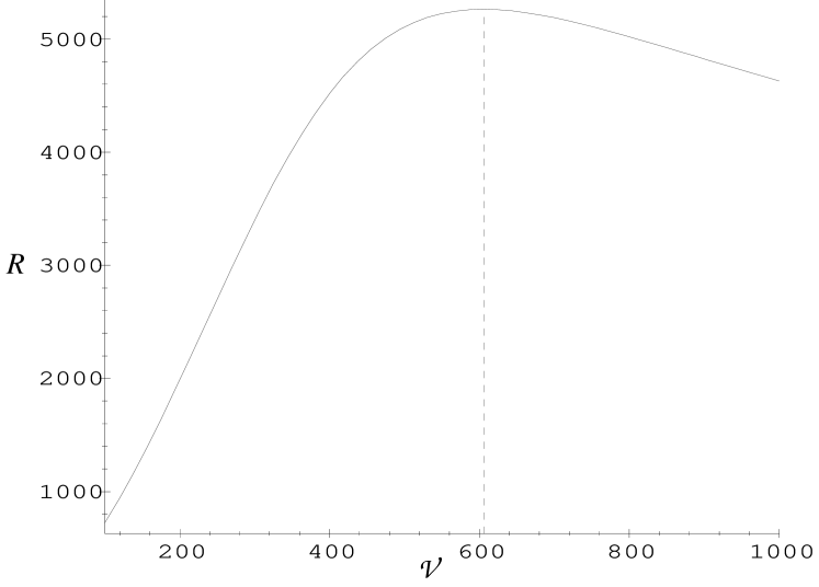
Figure 3: Function $R({\cal V})$ characterising effectiveness of separation of two different contaminants for parameters given in Table 1.

Then the optimal regime of two species separation gives

$$\frac{\Delta T}{\delta} = \frac{6^{1/8}}{2}\sqrt{\frac{3L}{b}}\frac{\Delta\kappa}{\kappa}{\cal U}^{1/4}$$ (45)

$${}\times\left[1-6^{1/4}\frac{7}{24}{\cal U}^{-1/2}-\frac{1997}{384}\sqrt{\frac{2}{3}}{\cal U}^{-1}+{\cal O}\left({\cal U}^{-3/2}\right)\right]\,.$$

For the geometry of the channel considered in [14] and parameters given in Table 1 the maximum resolution is thus

$$\frac{\Delta T}{\delta}\approx 430\frac{\Delta\kappa}{\kappa}\,,$$ (46)

where $\delta\approx 1$ min. For the regime considered the time necessary for the contaminant to travel a distance $L=50\,\mbox{cm}$ is $T\approx 14.2$ hours—probably too long to be practical. A suggestion is to reduce the channel length or increase the longitudinal flow speed, while increasing the cross-flow velocity to be closer to the optimum.

Acknowledgement

We thank the Australian Research Council for a grant supporting this research, and Dr Bob Anderssen of CSIRO for introducing us to this problem.

Appendix A Computer algebra handles all the details

Just one of the virtues of this centre manifold approach to modelling is that it is systematic. This enables relatively straightforward computer programs to be written to find the centre manifold and the evolution thereon [12, e.g.].

For this problem the iterative algorithm is implemented by a computer algebra program written in reduce Although there are many details in the program, the correctness of the results are only determined by driving to zero (line 48) the residual of the governing differential equation, evaluated on line 41, to the error specified on line 38 and with boundary and amplitude conditions checked on lines 50–52. The other details only affect the rate of convergence to the ultimate answer.

COMMENT Use iteration to form the centre manifold model of shear
dispersion in a channel with a constant cross-flow of velocity -v.
Flow between y=0 and y=V where V=(b v)/k, rsig=k/nu, A=(v/u*)^2,
u*=-1/2 dp/dx (b k)/(rho nu v).  The centre manifold is parameterized
with c(x,0,t) such that the corrections satisfy c'(x,0,t)=0,
dc'(x,0,t)/dy=0 ;
% formating for printed output
on div; off allfac; on revpri; factor ev,rsig,df,a;
% ev(y) denotes exp(-y)
operator ev;
let { df(ev(y),y)=>-ev(y), ev(0)=>1, ev(V)=>ep};
ep:=1-1/m;
% operator for solvability, where m=1/(1-exp(-V))
operator intv;linear intv;
let { intv(1,y) => V
    , intv(y,y) => V^2/2
    , intv(y^~q,y) => V^(q+1)/(q+1)
    , intv(y^~q*ev(y),y)=>-V^q*ep+q*intv(y^(q-1)*ev(y),y)
    , intv(y*ev(y),y)=> 1-(1+V)*ep
    , intv(ev(y),y)=> 1/m };
% operator to solve d^2h/dy^2+dh/dy = rhs
operator linv;linear linv;
let{linv(1,y) =>  y-1+ev(y),
    linv(y,y) =>  -y+y^2/2+1-ev(y),
    linv(y^~q,y)=>y^(q+1)/(q+1)-q*linv(y^(q-1),y),
    linv(ev(y),y)=>-(y+1)*ev(y)+1,
    linv(y*ev(y),y)=>-(y^2/2+y+1)*ev(y)+1,
    linv(y^~q*ev(y),y)=>-y^(q+1)/(q+1)*ev(y)+q*linv(y^(q-1)*ev(y),y)};
% linear solution and velocity profile
depend c,x,t;
let df(c,t)=>g;
% u:=-2/rsig/V*(y-V*(1-exp(-y*rsig))/(1-exp(-V*rsig)));
u:=y*(y-V)*(2*y-6/rsig-V)*rsig/6/V;
h:=c*ev(y);
g:=0;
% iteration, for small d/dx and small reciprocal Prandtl number
let {df(c,x,~q)=>0 when q>2, rsig^2=>0};
m:=1; % optionally neglect e^(-V) terms
repeat begin
   eqn:=df(h,t)+u*df(h,x)-df(h,y)-df(h,y,2)-df(h,x,2)*K^2;
   % solvability
   gd:=-intv(eqn,y)*m;
   g:=g+gd;
   % concentration field
   h:=h+linv(eqn+gd*ev(y),y);
   showtime;
end until (eqn=0);
% confirm boundary and amplitude conditions
eqn:=sub(y=0,h+df(h,y));
eqn:=sub(y=V,h+df(h,y));
eqn:=sub(y=0,h)-c;
% output to file
off nat; on list; out "sffp.out";
cmean:=intv(h,y)/V; g:=g; h:=h;
shut "sffp.out"; on nat;
showtime;
end;

Appendix B Weak and moderate cross-flows

For completeness we record here the model for the case of relatively slow cross-flow, or equivalently of relatively high diffusivity. This provides results for all parameters ${\cal V}$, not just the large values described earlier.

The non-dimensionalisation used in the main body of this paper is inappropriate in the case of small cross-flow rates. At higher rates the contaminant is restricted to the boundary layer, but in low cross-flow it is spread over the channel height. Thus in the case of weak cross-flows we adopt the following scalings typical of those used for shear dispersion [8, 16, e.g.]:

$$y^{*}=\frac{y}{b}\,,\quad t^{*}=\frac{\kappa t}{b^{2}}\,,\quad x^{*}=\frac{x\kappa}{{{\bar{u}}}b^{2}}\,,\quad u^{*}=\frac{u}{{{\bar{u}}}}\,,\quad v^{*}=\frac{bv}{\kappa}\,,\quad p^{*}=\frac{p}{\rho{\bar{u}}^{2}\sigma}\,.$$ (47)

Quantities are scaled: $y$ with the channel width; $t$ with a cross-channel diffusion time, $\tau=b^{2}/\kappa\approx 1.25\times 10^{4}$ sec; $x$ with the downstream advection distance in a cross-channel diffusion time, $\xi={{\bar{u}}}\tau\approx 1.25\times 10^{3}$ cm; $u$ with the mean downstream velocity; and $v$ with a cross-stream diffusion speed, $\kappa/b\approx 4\times 10^{-4}$ cm/s. As before ${\cal V}=v_{0}b/\kappa$ is the main parameter and is used to denote a non-dimensional cross-flow velocity, though it may well be thought of as an effective channel width, or as the inverse of the molecular diffusivity.

Then after substituting (47) into the Navier-Stokes and continuity equations (4)–(5) and dropping stars the equation for the steady horizontal velocity component $u(y)$ becomes

$$-\frac{{\cal V}}{\sigma}\frac{\partial u}{\partial y}=12+\frac{\partial^{2}u}{\partial y^{2}}\,,\quad\mbox{s.t.}\quad u=0\quad\mbox{at $y=0$ and $y=1$}$$ (48)

with the nearly parabolic solution

$$u(y) = \frac{12\sigma}{{\cal V}}\left(\frac{1-e^{-{\cal V}y/\sigma}}{1-e^{-{\cal V}/\sigma}}-y\right)\,$$ (49)

$$= y(1-y)\left(6+(1-2y)\frac{{\cal V}}{\sigma}+{\cal O}\left(\frac{{\cal V}^{2}}{\sigma^{2}}\right)\right)\,.$$

The advection-diffusion equation for the contaminant becomes

$$\frac{\partial c}{\partial t}+u\frac{\partial c}{\partial x}-{\cal V}\frac{\partial c}{\partial y}=\frac{\partial^{2}c}{\partial y^{2}}+\frac{1}{{\cal U}^{2}}\frac{\partial^{2}c}{\partial x^{2}}\,,$$ (50)

where ${\cal U}={\bar{u}}b/\kappa$ is a downstream Peclet number as before, and with boundary conditions

$${\cal V}c+\frac{\partial c}{\partial y}=0\quad\mbox{at $y=0$ and $y=1$.}$$ (51)

In the absence of any $x$-variations the steady solution is

$$c_{0}=Ce^{-{\cal V}y}\,,$$ (52)

where as before $C=c(x,0,t)$ is the concentration of the contaminant at the lower plate. The other $x$-independent solutions, all decaying, are

$$c_{n}=C_{n}\left[{\cal V}\sin\left(n\pi y\right)-2n\pi\cos\left(n\pi y\right)\right]\exp\left(-\frac{{\cal V}y}{2}+\lambda_{n}t\right)\,,$$ (53)

for $n=1,2,\ldots$ where the decay rate is

$$\lambda_{n}=-\frac{{\cal V}^{2}}{4}-n^{2}\pi^{2}\,.$$ (54)

For small ${\cal V}$ the decay is dominated by the second term above due to cross-channel diffusion. The slowest rate of decay to the centre manifold comes from the $n=1$ mode. Using arguments similar to those given in Section 3 we deduce that in the case of small cross-flow rates $C_{1}\propto 1$ and, consequently, the dimensional decay time is expected to be $\tau/|\lambda_{1}|\approx\tau/\pi^{2}\approx 20$ min which is an order of magnitude larger than that for the strong cross-flows considered earlier. This reaffirms the existence of an attractive centre manifold for slowly varying solutions, albeit attractive on a larger time scale.

As before, an iterative procedure was implemented in computer (not listed) to solve the contaminant transport equations (50)–(51) by finding the centre manifold and the evolution thereon (22). The resulting expression for the concentration field is

$$c = Ce^{-{\cal V}y}+12\frac{\partial C}{\partial x}\frac{m-1}{{\cal V}^{3}}\left(1-\frac{1}{\sigma}\right)\left(1-e^{-{\cal V}y}(1+{\cal V}y)\right)$$ (55)

$${}+\frac{\partial C}{\partial x}\frac{y^{2}}{{\cal V}^{2}}e^{-{\cal V}y}\left[(6-3{\cal V}+2{\cal V}y)\left(1-\frac{1}{\sigma}\right)-\frac{{\cal V}^{2}}{2\sigma}(1-y)^{2}\right]$$

$${}+{\cal O}\left(\frac{\partial^{2}C}{\partial x^{2}},\sigma^{-2}\right)\,.$$

The general expressions for the coefficients of the evolution equation (33) are quite involved and for brevity here we neglect terms inversely proportional to the Prandtl number $\sigma$ since it is typically small ($\sigma\approx 5\times 10^{4}$ for example):

$$U = \frac{6}{{\cal V}}(2m-1)-\frac{12}{{\cal V}^{2}}+{\cal O}\left(\sigma^{-1}\right)\,,$$ (56)

$$D = \frac{1}{{\cal U}^{2}}+24m\frac{e^{-{\cal V}}}{{\cal V}^{2}}-144m^{2}(2m-1)\frac{e^{-{\cal V}}}{{\cal V}^{3}}-72\frac{4m^{2}e^{-{\cal V}}-1}{{\cal V}^{4}}$$ (57)

$${}-720\frac{2m-1}{{\cal V}^{5}}+\frac{2016}{{\cal V}^{6}}+{\cal O}\left(\sigma^{-1}\right)\,,$$

$$E = -24m^{2}(2m-1)\frac{e^{-{\cal V}}}{{\cal V}^{3}}+\frac{432}{5}m^{2}\left(20m^{2}e^{-{\cal V}}+3\right)\frac{e^{-{\cal V}}}{{\cal V}^{4}}$$ (58)

$${}-6912m^{4}(2m-1)\frac{e^{-2{\cal V}}}{{\cal V}^{5}}-24192m^{4}\frac{e^{-2{\cal V}}}{{\cal V}^{6}}$$

$${}-864(2m-1)\frac{58m^{2}e^{-2{\cal V}}+5}{{\cal V}^{7}}-5184\frac{48m^{2}e^{-{\cal V}}-17}{{\cal V}^{8}}$$

$${}-642816\frac{2m-1}{{\cal V}^{9}}+\frac{1672704}{{\cal V}^{10}}+{\cal O}\left(\sigma^{-1}\right)\,,$$

$$F = 16m^{2}\left(6m^{2}e^{-{\cal V}}+1\right)\frac{e^{-{\cal V}}}{{\cal V}^{4}}-\frac{1152}{5}m^{2}(2m-1)\left(15m^{2}e^{-{\cal V}}+1\right)\frac{e^{-{\cal V}}}{{\cal V}^{5}}$$ (59)

$${}+\frac{288}{35}m^{2}(2m-1)\left(168m^{2}(100m^{2}e^{-{\cal V}}+21)e^{-{\cal V}}+37\right)\frac{e^{-{\cal V}}}{{\cal V}^{6}}$$

$${}-1152m^{2}(2m-1)\left(24m^{2}\left(15m^{2}e^{-{\cal V}}-1\right)e^{-{\cal V}}-1\right)\frac{e^{-{\cal V}}}{{\cal V}^{7}}$$

$${}-\frac{6912}{5}m^{2}\left(60m^{2}\left(25m^{2}e^{-{\cal V}}-2\right)e^{-{\cal V}}-79\right)\frac{e^{-{\cal V}}}{{\cal V}^{8}}$$

$${}-6912m^{2}(2m-1)\left(630m^{2}e^{-{\cal V}}+17\right)\frac{e^{-{\cal V}}}{{\cal V}^{9}}$$

$${}-13824\frac{m^{2}\left(1806m^{2}e^{-{\cal V}}+197\right)e^{-{\cal V}}-33}{{\cal V}^{10}}$$

$${}-518400(2m-1)\frac{106m^{2}e^{-{\cal V}}+29}{{\cal V}^{11}}-829440\frac{463m^{2}e^{-{\cal V}}-237}{{\cal V}^{12}}$$

$${}-1208742912\frac{2m-1}{{\cal V}^{13}}+\frac{2947995648}{{\cal V}^{14}}+{\cal O}\left(\sigma^{-1}\right)\,.$$

Figure 4: The coefficients of the evolution equation (33) as functions of the cross-channel Peclet number ${\cal V}$ for the infinite Prandtl number $\sigma$.

These coefficients are plotted in Figure 4. All of them eventually decrease in magnitude with increasing cross-flow. The maximum of the effective diffusion coefficient $D$ is reached at ${\cal V}\approx 3$. Thus the “zone broadening” [7] associated with the dispersion of the contaminant affects the distribution of the contaminant at a greater degree when the cross-flow is relatively weak. The fourth order coefficient $F$ is negative for ${\cal V}<5$ and consequently equation (33), in contrast to the case of strong cross-flows reported in Section 4, predicts stable (decaying) in time evolution of the average concentration of the contaminant for all longitudinal wavenumbers.

The small ${\cal V}$ expansions of expressions (55)–(59) are

$$c = C\left[1-{\cal V}y+\frac{1}{2}{\cal V}^{2}y^{2}-\frac{1}{6}{\cal V}^{3}y^{3}\right]+\frac{\partial C}{\partial x}y^{2}\left[-\frac{1}{2}(y-1)^{2}\right.$$ (60)

$${}+\frac{{\cal V}y}{60}\left(24y^{2}-45y+20+\frac{1}{\sigma}\left(6y^{2}-15y+10\right)\right)$$

$${}+\frac{{\cal V}^{2}}{120}\left(20y^{4}-36y^{3}+15y^{2}-1-\frac{1}{\sigma}\left(10y^{4}-24y^{3}+15y^{2}+1\right)\right)$$

$${}\left.+\frac{{\cal V}^{3}y}{1260}\left(60y^{4}-105y^{3}+42y^{2}-7+\frac{1}{\sigma}\left(45y^{4}-105y^{3}+63y^{2}+7\right)\right)\right]$$

$${}+{\cal O}\left(\frac{\partial^{2}C}{\partial x^{2}},\sigma^{-2},{\cal V}^{4}\right)\,,$$

$$U = 1-\frac{{\cal V}^{2}}{60}+\frac{{\cal V}^{4}}{2520}-\frac{{\cal V}^{6}}{100800}+{\cal O}\left(\sigma^{-1},{\cal V}^{8}\right)\,,$$ (61)

$$D = \frac{1}{{\cal U}^{2}}+\frac{1}{210}\left(1+\frac{7}{60}{\cal V}^{2}-\frac{89}{7920}{\cal V}^{4}+\frac{239}{386100}{\cal V}^{6}\right)+{\cal O}\left(\sigma^{-1},{\cal V}^{8}\right),$$ (62)

$$E = \frac{1}{69300}\left(1+\frac{1073}{1365}{\cal V}^{2}-\frac{233}{910}{\cal V}^{4}+\frac{71629}{2570400}{\cal V}^{6}\right)+{\cal O}\left(\sigma^{-1},{\cal V}^{8}\right)\,,$$ (63)

$$F = -\frac{1}{2252250}\left(1-\frac{26879}{85680}{\cal V}^{2}+\frac{26341969}{68372640}{\cal V}^{4}+\frac{1187149277}{15041980800}{\cal V}^{6}\right)$$ (64)

$${}+{\cal O}\left(\sigma^{-1},{\cal V}^{8}\right)\,.$$

The expansions for large cross-flow ${\cal V}$ are

$$c = Ce^{-{\cal V}y}$$ (65)

$${}+\frac{\partial C}{\partial x}y^{2}e^{-{\cal V}y}\left[-\frac{1}{2\sigma}(y-1)^{2}+\left(\frac{2y-3}{{\cal V}}+\frac{6}{{\cal V}^{2}}\right)\left(1-\frac{1}{\sigma}\right)\right]$$

$${}+{\cal O}\left(\frac{\partial^{2}C}{\partial x^{2}},\sigma^{-2},e^{-{\cal V}}\right)\,,$$

$$U = \frac{6}{{\cal V}}\left(1-\frac{2}{{\cal V}}\right)+{\cal O}\left(\sigma^{-1},e^{-{\cal V}}\right)\,,$$ (66)

$$D = \frac{1}{{\cal U}^{2}}+\frac{72}{{\cal V}^{4}}\left(1-\frac{10}{{\cal V}}+\frac{28}{{\cal V}^{2}}\right)+{\cal O}\left(\sigma^{-1},e^{-{\cal V}}\right)\,,$$ (67)

$$E = -\frac{4320}{{\cal V}^{7}}\left(1-\frac{102}{5{\cal V}}+\frac{744}{5{\cal V}^{2}}-\frac{1936}{5{\cal V}^{3}}\right)+{\cal O}\left(\sigma^{-1},e^{-{\cal V}}\right)\,,$$ (68)

$$F = \frac{456192}{{\cal V}^{10}}\left(1-\frac{725}{22{\cal V}}+\frac{4740}{11{\cal V}^{2}}-\frac{29146}{11{\cal V}^{3}}+\frac{71084}{11{\cal V}^{4}}\right)+{\cal O}\left(\sigma^{-1},e^{-{\cal V}}\right).$$ (69)

The above expressions are equivalent to, but appear a little different from, the leading terms in expressions (30)–(32), (4) and (35) because of the different non-dimensionalisation. These large ${\cal V}$ expressions evidently give the behaviour of the coefficients for non-dimensional cross-flow ${\cal V}$ bigger than about 5–10.

References

- [1] J. Carr. Applications of centre manifold theory, volume 35 of Applied Math Sci. Springer-Verlag, 1981.
- [2] J. Carr and R.G. Muncaster. The application of centre manifold theory to amplitude expansions. I. ordinary differential equations. J. Diff. Eqns., 50:260–279, 1983.
- [3] J. Carr and R.G. Muncaster. The application of centre manifold theory to amplitude expansions. II. infinite dimensional problems. J. Diff. Eqns, 50:280–288, 1983.
- [4] P.H. Coullet and E.A. Spiegel. Amplitude equations for systems with competing instabilities. SIAM J. Appl. Math., 43:776–821, 1983.
- [5] J.C. Giddings. Crossflow gradients in thin channels for separation by hyperlayer FFF, SPLITT cells, elutrition, and related methods. Separation Sci & Tech, 21:831–843, 1986.
- [6] A. Litzén. Separation speed, retention, and dispersion in asymmetrical flow field-flow fractionation as functions of channel dimensions and flow rates. Anal. Chem., 65:461–470, 1993.
- [7] A. Litzén and K.-G. Wahlund. Zone broadening and dilution in rectangular and trapezoidal asymmetrical flow field-flow fractionation channels. Anal. Chem., 62:1001–1007, 1990.
- [8] G.N. Mercer and A.J. Roberts. A centre manifold description of contaminant dispersion in channels with varying flow properties. SIAM J. Appl. Math., 50:1547–1565, 1990.
- [9] G.N. Mercer and A.J. Roberts. A complete model of shear dispersion in pipes. Jap. J. Indust. Appl. Math., 11:499–521, 1994.
- [10] A.J. Roberts. The application of centre manifold theory to the evolution of systems which vary slowly in space. J. Austral. Math. Soc. B, 29:480–500, 1988.
- [11] A.J. Roberts. Low-dimensional modelling of dynamical systems. preprint, USQ, February 1997.
- [12] A.J. Roberts. Low-dimensional modelling of dynamics via computer algebra. Comput. Phys. Comm., 100:215–230, 1997.
- [13] M.R. Schure, B.N. Barman, and J.G. Giddings. Deconvolution of nonequilibrium band broadening effects for accurate particle size distributions by sedimentation field-flow fractionation. Anal. Chem., 61:2735–2743, 1989.
- [14] K.-G. Wahlund and J.G. Giddings. Properties of an asymmetrical flow field-flow fractionation channel having one permeable wall. Anal. Chem., 59:1332–1339, 1987.
- [15] S.D. Watt and A.J. Roberts. The construction of zonal models of dispersion in channels via matching centre manifolds. J. Austral. Maths. Soc. B, 38:101–125, 1994.
- [16] S.D. Watt and A.J. Roberts. The accurate dynamic modelling of contaminant dispersion in channels. SIAM J Appl Math, 55(4):1016–1038, 1995.
- [17] P.J. Wyatt. Submicrometer particale sizing by multiangle light scattering following fractionation. J. Colloid & Interface Sci., 197:9–20, 1998.