Holistic finite differences ensure fidelity to Burger’s equation

Abstract

I analyse a generalised Burger’s equation to develop an accurate finite difference approximation to its dynamics. The analysis is based upon centre manifold theory so we are assured that the finite difference model accurately models the dynamics and may be constructed systematically. The trick to the application of centre manifold theory is to divide the physical domain into small elements by introducing insulating internal boundaries which are later removed. Burger’s equation is used as an example to show how the concepts work in practise. The resulting finite difference models are shown to be significantly more accurate than conventional discretisations, particularly for highly nonlinear dynamics. This centre manifold approach treats the dynamical equations as a whole, not just as the sum of separate terms—it is holistic. The techniques developed here may be used to accurately model the nonlinear evolution of quite general spatio-temporal dynamical systems.

1 Introduction

I introduce a new approach to finite difference approximation by illustrating the concepts and analysis on the definite example of a generalised Burger’s equation. In some non-dimensional form we take the following partial differential equation (pde) to govern the evolution of $u(x,t)$:

$$\frac{\partial u}{\partial t}+\alpha u\frac{\partial u}{\partial x}=\frac{\partial^{2}u}{\partial x^{2}}-\beta u^{3}\,.$$ (1)

This example equation, which includes the mechanisms of dissipation, $u_{xx}$, and nonlinear advection/steepening, $\alpha uu_{x}$, generalises Burger’s equation by also including a nonlinear damping, $\beta u^{3}$. Consider implementing the method of lines by discretising in $x$ and integrating in time as a set of ordinary differential equations. A finite difference approximation to (1) on a regular grid in $x$ is straightforward, say $x_{j}=jh$ for some grid spacing $h$. For example, the linear term

$$\frac{\partial^{2}u}{\partial x^{2}}=\frac{u_{j+1}-2u_{j}+u_{j-1}}{h^{2}}+{\cal O}\left(h^{2}\right)\,.$$

However, there are differing valid alternatives for the nonlinear term $uu_{x}$: two possibilities are

$$u\frac{\partial u}{\partial x}=\frac{u_{j}(u_{j+1}-u_{j-1})}{2h}+{\cal O}\left(h^{2}\right)=\frac{u_{j+1}^{2}-u_{j-1}^{2}}{4h}+{\cal O}\left(h^{2}\right)\,.$$

Which is better? The answer depends upon how the discretisation of the nonlinearity interacts with the dynamics of other terms. The traditional approach of considering the discretisation of each term separately does not tell us. Instead, in order to find the best discretisation we have to consider the dynamics of all terms in the equation in a holistic approach.

Centre manifold theory (see the book by Carr [1]) has appropriate characteristics to do this. It addresses the evolution of a dynamical system in a neighbourhood of a marginally stable fixed point; based upon the linear dynamics the theory guarantees that an accurate low-dimensional description of the nonlinear dynamics may be deduced. The theory is a powerful tool for the modelling of complex dynamical systems [2, 3, 12, 13, 9, e.g.] such as dispersion [23, 11, 26, e.g.], thin fluid films [4, 17, 21, e.g.] and other applications discussed in the review [19]. Here we place the discretisation of a nonlinear pde such as (1) within the purview of centre manifold theory by the following artifice (such mathematical trickery has proven effective in thin fluid flows [17]). Introduce a parameter $\gamma$, $0\leq\gamma\leq 1$: at the midpoints of the grid, $x=(j+1/2)h$, insert artificial boundaries which are “insulating” when $\gamma=0$, but when $\gamma=1$ the boundaries ensure sufficient continuity to recover the original problem. In essence this divides the domain into equi-sized elements centred upon each grid point, say the domain is partitioned into $m$ elements. For (1) we may use

$$\frac{\partial u^{+}}{\partial x}=\frac{\partial u^{-}}{\partial x}\,,\quad(1-\gamma)\frac{h}{2}\left(\frac{\partial u^{+}}{\partial x}+\frac{\partial u^{-}}{\partial x}\right)=\gamma\left(u^{+}-u^{-}\right)\,,$$ (2)

where $u^{+}$ is just to the right of a midpoint and $u^{-}$ to the left. When $\gamma=1$ these reduce to conditions ensuring appropriate continuity between adjacent elements. When $\gamma=0$ they reduce to conditions equivalent to the insulating

$$\frac{\partial u^{+}}{\partial x}=\frac{\partial u^{-}}{\partial x}=0\,.$$

We treat terms multiplied by $\gamma$ as “nonlinear” perturbations to the insulated dynamics. Then in the “linear” dynamics governed by

$$\frac{\partial u}{\partial t}=\frac{\partial^{2}u}{\partial x^{2}}\,,$$

each element evolves exponentially quickly (in a time ${\cal O}\left(h^{2}\right)$) to a constant value, say $u=u_{j}$ in the $j$th element (the particular value depends upon the initial conditions). But in the presence of the perturbative influences of the nonlinear terms and the coupling between elements, the values $u_{j}$ associated with each element will evolve in time. This picture is the basis of centre manifold theory which is applied in Section 2 to assure three things:

• the existence of an $m$ dimensional centre manifold parameterized by $u_{j}$;

• the relevance of the $m$ dimensional dynamics as an accurate and stable model of the original dynamics (1) (sometimes called asymptotic completeness [22] or [5]);

• and that we may approximate the shape of the centre manifold and the evolution thereon by approximately solving an associated pde.

These dynamics on the centre manifold form a finite difference approximation. For example, the analysis in Section 3 of the generalised Burger’s equation (1) is unequivocally in favour of the discretisation

$$\dot{u}_{j}+\alpha u_{j}\left[\frac{u_{j+1}-u_{j-1}}{2h}-\frac{\alpha u_{j}}{12}(u_{j+1}-2u_{j}+u_{j-1})\right]$$

$$\approx\frac{u_{j+1}-2u_{j}+u_{j-1}}{h^{2}}$$

$${}-\frac{\beta}{24}\left(u_{j-1}^{3}+3u_{j-1}u_{j}^{2}+16u_{j}^{3}+3u_{j+1}u_{j}^{2}+u_{j+1}^{3}\right)\,,$$ (3)

as an early approximation ($\dot{u}_{j}$ denotes $du_{j}/dt$). Provided the initial conditions are not too extreme, centre manifold theory assures us that such a discretisation models the dynamics of (1) to errors ${\cal O}\left(\|u\|^{4}\right)$. Observe that it is best to discretise the nonlinear $uu_{x}$ terms directly, but that there is a nonlinear correction involving the second difference. Further, the cubic nonlinearity is discretised in a non-obvious complicated form. Margolin & Jones [10] have previously applied inertial manifold ideas to discretisations of Burger’s equation. However, they used just two basis functions on each element and invoked the adiabatic approximation for time derivatives of “slaved” modes. Here I allow arbitrarily convoluted dependence within each element and include all effects of time variations. The methodology presented here provides a rigorous approach to finite difference models.

The discretisation (3) is just a low-order approximation, centre manifold theory provides systematic corrections. For example, Equation (3) is obtained from terms linear in the coupling $\gamma$. Analysis including quadratic terms in $\gamma$ leads to the fourth-order accurate model discussed in Section 4. Analysis to higher orders in the nonlinearity, discussed in Section 3, shows higher order corrections to the discretisation of the nonlinear terms and also incorporates effects from a coupling of the different nonlinearities.

Computer algebra is an effective tool for modelling because of the systematic nature of centre manifold theory [14, 8, 20]. The specific finite difference models presented here were derived by the computer algebra program given in Appendix A. Such a computer algebra program may be straightforwardly modified to model more complicated dynamical systems.

In this work I concentrate upon a proof of the concept of applying centre manifold theory to constructing effective finite difference models. To that end we only consider an infinite domain or strictly periodic solutions in finite domains. Then all elements of the discretisation are identical by symmetry and the analysis of all elements is simultaneous. However, if physical boundaries to the domain of the pde are present, then those elements near the physical boundary will need special treatment. I do not see the need for any new concepts, just an increase in the amount of detail. The centre manifold approach also sheds an interesting light upon the issue of the initial condition for a finite difference approximation. Earlier work on the issue of initial conditions in general [16, 7, 18] hints that the initial values for the parameters $u_{j}(t)$ is not simply the field $u$ sampled at the grid points, $u(x_{j},0)$, but some more subtle transform. Some preliminary research suggests that a leading order approximation is that $u_{j}(0)$ is the element average of $u(x,0)$, an approximation which usefully conserves $u$. Lastly, here we have only analysed an autonomous dynamical system, the pde (1); forcing applied to the pde may be approximated using the projection obtained for initial conditions [6, 18]. Further research is needed in the above issues and in the application of the theory to higher order pdes and in higher spatial dimensions.

2 Centre manifold theory underpins the fidelity

Here I describe in detail one way to place the discretisation of pdes within the purview of centre manifold theory. For definiteness I address the generalised Burger’s equation (1) as an example of a broad class of pdes.

As introduced earlier, the discretisation is established via an equi-spaced grid of collocation points, $x_{j}=jh$ say, for some constant spacing $h$. At midpoints $x_{j+1/2}=(x_{j}+x_{j+1})/2$ artificial boundaries are introduced with one extra refinement over that discussed in the Introduction:

$$\frac{\partial u^{+}}{\partial x}=\frac{\partial u^{-}}{\partial x}\,,$$ (4)

$$(1-\gamma){\cal A}\frac{h}{2}\left(\frac{\partial u^{+}}{\partial x}+\frac{\partial u^{-}}{\partial x}\right)=\gamma\left(u^{+}-u^{-}\right)\,,$$ (5)

where the introduction of the near identity operator

$${\cal A}=1-\frac{h^{2}}{12}\frac{\partial}{\partial t}+\frac{h^{4}}{120}\frac{\partial^{2}}{\partial t^{2}}-\frac{17h^{6}}{20160}\frac{\partial^{3}}{\partial t^{3}}+\cdots\,,$$ (6)

will be explained in the next section. These boundaries divide the domain into a set of elements, the $j$th element centred upon $x_{j}$ and of width $h$. A non-zero value of the parameter $\gamma$ couples these elements together so that when $\gamma=1$ the pde is effectively restored over the whole domain. The generalised Burger’s equation (1) with “internal boundary conditions” (4–5) is analysed here to give the discretisation in the interior of the domain.

The application of centre manifold theory is based upon a linear picture of the dynamics. Adjoin the dynamically trivial equation

$$\frac{\partial\gamma}{\partial t}=0\,,$$ (7)

and consider the dynamics in the extended state space $(u(x),\gamma)$. This is a standard trick used to unfold bifurcations [1, §1.5] or to justify long-wave approximations [15]. Within each element $u=\gamma=0$ is a fixed point. Linearized about each fixed point, that is to an error ${\cal O}\left(\|u\|^{2}+\gamma^{2}\right)$, the pde is

$$\frac{\partial u}{\partial t}=\frac{\partial^{2}u}{\partial x^{2}}\,,\quad\mbox{s.t.}\quad{\cal A}\left.\frac{\partial u}{\partial x}\right|_{x=x_{j\pm 1/2}}=0\,,$$

namely the diffusion equation with essentially insulating boundary conditions. There are thus linear eigenmodes associated with each element:

$$\gamma=0\,,\quad u\propto\left\{\begin{array}[]{ll}e^{\lambda_{n}t}\cos[n\pi(x-x_{j-1/2})/h]\,,&x_{j-1/2}<x<x_{j+1/2}\,,\\ 0\,,&\mbox{otherwise}\,,\end{array}\right.$$ (8)

for $n=0,1,\ldots$, where the decay rate of each mode is

$$\lambda_{n}=-\frac{n^{2}\pi^{2}}{h^{2}}\,;$$ (9)

together with the trivial mode $\gamma=\mbox{const}$, $u=0$. In a domain with $m$ elements, evidentally all eigenvalues are negative, $-\pi^{2}/h^{2}$ or less, except for $m+1$ zero eigenvalues: $1$ associated with each of the $m$ elements and $1$ from the trivial (7). Thus, provided the nonlinear terms in (1) are sufficiently well behaved, the existence theorem ([3, p281] or [25, p96]) guarantees that a $m+1$ dimensional centre manifold ${\cal M}$ exists for (1) with (4–7). The centre manifold ${\cal M}$ is parameterized by $\gamma$ and a measure of $u$ in each element, say $u_{j}$: using $u$ to denote the collection of such parameters, ${\cal M}$ is written as

$$u(x,t)=v(x;\mbox{\boldmath$u$},\gamma)\,.$$ (10)

In this the analysis has a very similar appearance to that of finite elements. The theorem also asserts that on the centre manifold the parameters $u_{j}$ evolve deterministically

$$\dot{u}_{j}=g_{j}(\mbox{\boldmath$u$},\gamma)\,,$$ (11)

where $g_{j}$ is the restriction of (1) and (4–7) to ${\cal M}$. In this approach the parameters of the description of the centre manifold may be anything that sensibly measures the size of $u$ in each element—I simply choose the value of $u$ at the grid points, $u_{j}=u(x_{j},t)$. This provides the necessary amplitude conditions, namely that

$$u_{j}=v|_{x_{j}}\,.$$ (12)

The above application of the theorem establishes that in principle we may find the dynamics (11) of the interacting elements of the discretisation. A low order approximation is given in (3).

The next outstanding question to answer is: how can we be sure that such a description of the interacting elements does actually model the dynamics of the original system (1) with (4–7)? In the development of inertial manifolds by Temam [24] and others, this question is sometimes phrased as one about the asymptotic completeness of the model, for example see Robinson [22] or Constantin et al [5, Chapt.12–3]. Here, the relevance theorem of centre manifolds, [3, p282] or [25, p128], guarantees that all solutions of (1) and (4–7) which remain in the neighbourhood of the origin in $(u(x),\gamma)$ space are exponentially quickly attracted to a solution of the $m$ finite difference equations (11). For practical purposes the rate of attraction is estimated by the leading negative eigenvalue, here $-\pi^{2}/h^{2}$. Centre manifold theory also guarantees that the stability near the origin is the same in both the model and the original. Thus the finite difference model will be stable if the original dynamics are stable. After exponentially quick transients have died out, the finite difference equation (11) on the centre manifold accurately models the complete system (1) and (4–7).

The last piece of theoretical support tells us how to approximate the shape of the centre manifold and the evolution thereon. Approximation theorems such as that by Carr & Muncaster [3, p283] assure us that upon substituting the ansatz (10–11) into the original (1) and (4–7) and solving to some order of error in $\|u\|$ and $\gamma$, then ${\cal M}$ and the evolution thereon will be approximated to the same order. The catch with this application is that we need to evaluate the approximations at $\gamma=1$ because it is only then that the artificial internal boundaries are removed. In some applications of such an artificial homotopy I have demonstrated good convergence in the parameter $\gamma$ [17]. Thus although the order of error estimates do provide assurance, the actual error due to the evaluation at $\gamma=1$ should be also assessed otherwise. Here, as discussed in Section 4, we have crafted the interaction (5) between elements so that low order terms in $\gamma$ recover the exact finite difference formula for linear terms. Note that although centre manifold theory “guarantees” useful properties near the origin in $(u(x),\gamma)$ space, because of the need to evaluate asymptotic expressions at $\gamma=1$, I have used a weaker term elsewhere, namely “assures”.

3 Numerical comparisons show the effectiveness

We now turn to a detailed description of the centre manifold model for Burger’s equation (1).

The algebraic details of the derivation of the centre manifold model (10–11) is the task of the computer algebra program listed in the Appendix. In an algorithm introduced in [20], the program iterates to drive to zero the residuals of the governing differential equation (1) and its boundary conditions (4–5). A key part of the iteration is to solve for corrections $v^{\prime}$ and $g^{\prime}$ from the linear diffusion equation within each element

$$\frac{\partial^{2}v^{\prime}}{\partial x^{2}}=g^{\prime}+R\,,\quad\left.\frac{\partial v^{\prime}}{\partial x}\right|_{x_{j\pm 1/2}}=R_{\pm}\,,$$

where $R$ and $R_{\pm}$ denote the residuals for the current approximation. The initial approximation is simply that in each element $u=u_{j}$, constant, with $\dot{u}_{j}=g_{j}=0$. The algebraic details of this iteration are largely immaterial so long as the residuals iterate to zero to some order in $u$ and $\gamma$. This is achieved by the listed computer algebra program, it is included to replace the recording of tedious details of elementary algebra.

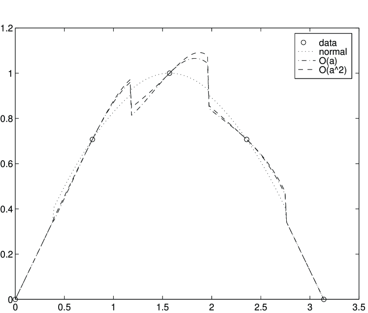
Figure 1: low order approximations (13) to the centre manifold field $u(x)$ within each element for a fixed set of data points (circles) corresponding to $m=8$ intervals on $[0,2\pi)$ with parameters $\alpha=6$, $\beta=0$ and $\gamma=1$: $\cdots$, the normal field associated with finite differences; $-\cdot-\cdot-$, includes the first effects of the nonlinear advection term, $\alpha uu_{x}$; $-~{}-~{}-$, includes the second-order effects in $\alpha$.

The shape of the centre manifold gives the field $u$ as a function of the parameters $u_{j}$ and the coupling $\gamma$. To low-order in $u$ and $\gamma$, and written in terms of the scaled coordinate $\xi=(x-x_{j})/h$, the solution field in the $j$th element is

$$u = u_{j}+\gamma\left[\frac{u_{j+1}-u_{j-1}}{2}\xi+\frac{u_{j+1}-2u_{j}+u_{j-1}}{2}\xi^{2}\right]$$ (13)

$${}+h\gamma\left[\alpha u_{j}(u_{j+1}-2u_{j}+u_{j-1})\left(\frac{1}{6}\xi^{3}-\frac{1}{8}\xi\right)\right]$$

$${}+h^{2}\gamma\left[\alpha^{2}u_{j}^{2}(u_{j+1}-2u_{j}+u_{j-1})\left(\frac{1}{24}\xi^{4}-\frac{1}{48}\xi^{2}\right)\right.$$

$$\quad\left.{}+\beta(u_{j+1}^{3}-3u_{j+1}u_{j}^{2}+4u_{j}^{3}-3u_{j-1}u_{j}^{2}+u_{j-1}^{3})\left(-\frac{1}{24}\xi^{4}-\frac{1}{48}\xi^{2}\right)\right.$$

$$\quad\left.{}+\beta(u_{j+1}^{3}-3u_{j+1}u_{j}^{2}+3u_{j-1}u_{j}^{2}-u_{j-1}^{3})\left(-\frac{1}{12}\xi^{3}+\frac{1}{48}\xi\right)\right.$$

$$\quad\left.{}-\beta\frac{u_{j}^{2}}{8}\left((u_{j+1}-u_{j-1})\xi+(u_{j+1}-2u_{j}+u_{j-1})\xi^{2}\right)\right]$$

$${}+{\cal O}\left(\|u\|^{4},\gamma^{2}\right)\,.$$

Observe the first line, when evaluated at $\gamma=1$, is simply the quadratic interpolant based upon second order accurate centred differences. This is normal finite differences. As displayed in Figure 1, the second line shows that this field should be modified because of the nonlinear advection term $\alpha uu_{x}$; the modification in proportion to the second difference at $x_{j}$ is reasonable because when $u$ has a local maximum the field must be decreased/increased to the left/right due to the advection to the right of the lower/higher levels of $u$ respectively. Note that the same discretisation for this nonlinear term is obtained here whether we code it as $\alpha uu_{x}$ or $\alpha(u^{2})_{x}/2$—the centre manifold is independent of any valid change in the algebraic description of the dynamics. The third line gives the next order correction due to the nonlinear advection and is also displayed in Figure 1. The fourth, fifth and sixth lines show how the cubic nonlinearity, $\beta u^{3}$, modifies $u$ in the element because of its nonlinearly varying effect as a source or sink when the field $u$ itself varies. It might appear odd to introduce the dysfunctional behaviour between elements shown in Figure 1, but centre manifold theory reasonably assures us that it is appropriate for the nonlinear dynamics we wish to model. In short, the description of the centre manifold is based upon standard differencing formulae, but includes effects upon $u$ within each element due to the nonlinear processes that act in the continuum dynamics.

The finite difference model is given by the evolution on the centre manifold. To linear terms in $\gamma$ but to two orders higher in $\|u\|$ it is

$$\dot{u}_{j} = \frac{\gamma}{h^{2}}\left(u_{j+1}-2u_{j}+u_{j-1}\right)-\frac{\gamma\alpha}{2h}u_{j}(u_{j+1}-u_{j-1})-\beta u_{j}^{3}$$ (14)

$${}+\gamma\left[\frac{\alpha^{2}}{12}u_{j}^{2}(u_{j+1}-2u_{j}+u_{j-1})\right.$$

$$\left.\quad{}+\frac{\beta}{24}\left(-u_{j+1}^{3}-3u_{j+1}u_{j}^{2}+8u_{j}^{3}-3u_{j-1}u_{j}^{2}-u_{j-1}^{3}\right)\right]$$

$${}+h\gamma\left[\frac{\alpha\beta}{8}u_{j}^{3}(u_{j+1}-u_{j-1})\right]$$

$${}+h^{2}\gamma\left[-\frac{\alpha^{4}}{720}u_{j}^{4}(u_{j+1}-2u_{j}+u_{j-1})\right.$$

$$\left.\quad{}+\frac{\alpha^{2}\beta}{5760}u_{j}^{2}\left(9u_{j+1}^{3}-113u_{j+1}u_{j}^{2}+208u_{j}^{3}-113u_{j-1}u_{j}^{2}+9u_{j-1}^{3}\right)\right.$$

$$\left.\quad{}+\frac{\beta^{2}}{1920}\left(-21u_{j+1}^{5}+6u_{j+1}^{3}u_{j}^{2}+7u_{j+1}u_{j}^{4}+16u_{j}^{5}\right.\right.$$

$$\left.\left.\qquad{}+7u_{j-1}u_{j}^{4}+6u_{j-1}^{3}u_{j}^{2}-21u_{j-1}^{5}\right)\phantom{\frac{1}{1}}\right]$$

$${}+{\cal O}\left(\|u\|^{6},\gamma^{2}\right)\,.$$

The first line recorded here, when evaluated for $\gamma=1$, is just the classic second-order finite difference equation for the generalised Burger’s equation (1). The second line starts accounting systematically for the variations in the field $u$ within each element and how they affect the evolution through the nonlinear terms. The approximation formed by the first three lines is that reported in the Introduction as (3). The fourth and further lines above, through $\alpha\beta$ and $\alpha^{2}\beta$ effects, show that this approach also accounts for interaction between the nonlinear terms in the pde in the finite difference approximation. Finite difference equations derived via this approach holistically model all the interacting dynamics of the entire pde.

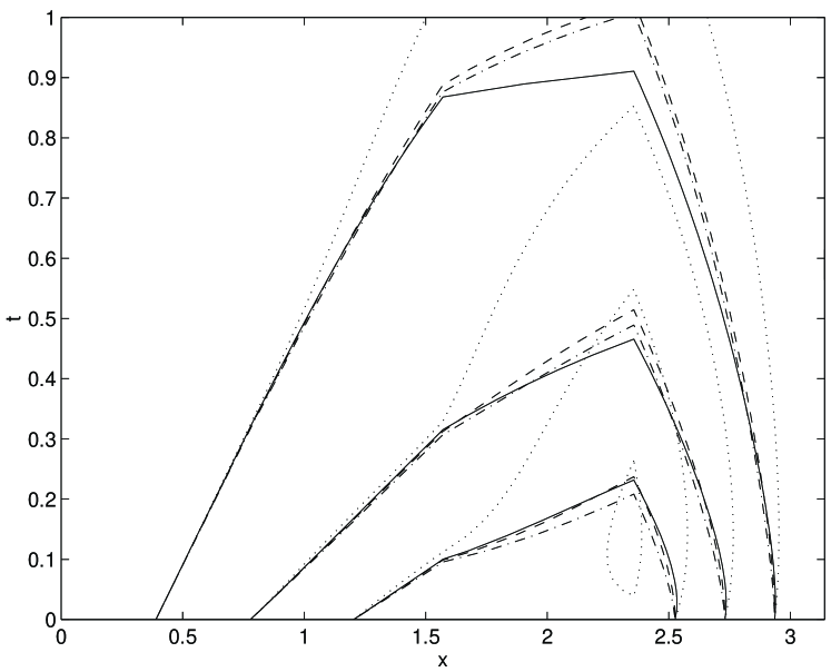
Figure 2: Contours of an exact solution $u(x,t)$, —–, to compare with numerical approximations (15): $\cdots$, the conventional approximation, errors $o(\alpha)$; $-\cdot-\cdot-$, the first correction, errors $o(\alpha^{2})$; $-~{}-~{}-$, the second correction, errors $o(\alpha^{4})$. Burger’s equation (1) with parameters $\alpha=6$ and $\beta=0$ is discretised on $m=8$ elements in $[0,2\pi)$ and drawn with contour interval $\Delta u=0.2$.

To show the effectiveness of the approach I compare the finite difference model (14) to exact solutions of Burger’s equation (1) with $\beta=0$. Exact solutions are obtained via the Cole-Hopf transformation $u=-(2/\alpha)\phi_{x}/\phi$ by choosing $\phi(x,t)$ satisfying the diffusion equation $\phi_{t}=\phi_{xx}$. For example, here I choose $2\pi$-periodic functions

$$\phi=\frac{14}{\sqrt{t_{0}}}e^{-\pi^{2}/4t_{0}}+\sum_{k}\frac{1}{\sqrt{t+t_{0}}}\exp\left[-\frac{(x-k2\pi)^{2}}{4(t+t_{0})}\right]\,,$$

with $t_{0}=\pi/(4\sqrt{\alpha})$, chosen so that the initial state $u(x,0)$ is a rough approximation to $\sin(x)$. Note that consequently $\|u(x,0)\|\approx 1$. Choosing $m$ intervals on $[0,2\pi)$ gives an element length $h=2\pi/m$ and grid points $x_{j}=jh$ for $j=0,\ldots,m-1$. Because of the antisymmetry in $u(x,t)$ about $x=k\pi$, I only display the interval $[0,\pi]$. With $\beta=0$, there are three different approximations from (14), with $\gamma=1$, depending upon where the expansion is truncated in $\|u\|$ (or equivalently in $\alpha$):

$$\dot{u}_{j} \approx \frac{1}{h^{2}}\left(u_{j+1}-2u_{j}+u_{j-1}\right)-\frac{\alpha}{2h}u_{j}(u_{j+1}-u_{j-1})$$ (15)

$${}+\frac{\alpha^{2}}{12}u_{j}^{2}(u_{j+1}-2u_{j}+u_{j-1})$$

$${}-h^{2}\frac{\alpha^{4}}{720}u_{j}^{4}(u_{j+1}-2u_{j}+u_{j-1})\,.$$

Just the first line forms a model with $o(\alpha)$ errors (a normal finite difference approximation), the first two lines form a model with $o(\alpha^{2})$ errors, and all shown terms form the model with $o(\alpha^{4})$ errors. The solutions of these models over $0<t<1$ with $m=8$ and nonlinearity parameter $\alpha=6$ are shown in Figure 2. Observe that the leading approximation (dotted) is significantly in error whereas the next two refinements (dot-dashed and dashed) are reasonably accurate. Such accuracy is remarkable considering the high level of nonlinearity, $\alpha=6$, and the few points in the discretisation, $m=8$.

Table 1: Comparison of the errors $\varepsilon$, defined in (16), of the spatially second order model (15) at the two first truncations in the nonlinear parameter $\alpha$ for various grid subintervals $m$. Observe that the higher order model is significantly less sensitive to the nonlinearity.

	$m=8$		$m=16$		$m=32$
$\alpha$	$o(\alpha)$	$o(\alpha^{2})$	$o(\alpha)$	$o(\alpha^{2})$	$o(\alpha)$	$o(\alpha^{2})$
1	.0116	.0095	.0031	.0025	.0008	.0006
3	.0356	.0109	.0102	.0040	.0026	.0011
6	.0694	.0115	.0215	.0059	.0054	.0018
10	.0971	.0186	.0318	.0055	.0081	.0026

For an assessment of errors over a range of parameters I record in Table 1 the error

$$\varepsilon=\max_{t}\left(\frac{1}{m}\sum_{j}|\epsilon_{j}(t)|\right)\,,$$ (16)

where $\epsilon_{j}(t)$ is the difference between an approximation and the exact solution at the $j$th grid point. Observe the usual properties that the errors decrease with increasing spatial resolution $m$, and that the errors increase with increasing nonlinearity $\alpha$. Our interest lies more in the comparison between the $o(\alpha)$ and $o(\alpha^{2})$ models (here the $o(\alpha^{4})$ model is virtually indistinguishable from the $o(\alpha^{2})$ model). For small nonlinearity, $\alpha=1$, there is very little difference; presumably the errors are dominated by the second-order approximation of spatial derivatives. As the nonlinearity $\alpha$ increases, the error of the $o(\alpha)$ approximation increases roughly in proportion to $\alpha$, but the error of the $o(\alpha^{2})$ approximation grows much more slowly. We conclude, as centre manifold theory assures us, that the nonlinearly corrected $o(\alpha^{2})$ model more accurately captures the nonlinear dynamics of Burger’s equation.

4 Higher order approximations are more accurate

So far I have reported results only to first order in the coupling coefficient $\gamma$. Retaining higher orders in $\gamma$ gives higher order difference rules as the coupling between adjacent elements is always ameliorated by a power of $\gamma$. However, it is only with the specific coupling of (5) that the $2p+1$ width stencil, obtained by retaining terms in $\gamma^{p}$, attains $2p$th-order accuracy in the linear terms. Retaining $\gamma^{2}$ terms, for example, then gives a fourth-order model which also performs remarkably well, especially for larger nonlinearities.

The particular form of the artificial internal boundary condition (5) controls the flow of information between elements of the discretisation. When $\gamma=1$ the condition reduces to requiring the desired continuity: $u^{-}=u^{+}$ from the rightmost term and $u^{-}_{x}=u^{+}_{x}$ from (4) where, as before, the superscripts $\pm$ denote evaluation at the internal boundary of expressions from the right/left-hand elements respectively. But we have enormous freedom in choosing the $(1-\gamma)$-term in (5). Our first requirement is that when $\gamma=0$ it insulates the elements from each other so that the values of $u_{j}$ in each element are independent in the centre manifold analysis. This is achieved is conjunction with (4) by only involving $u^{-}_{x}+u^{+}_{x}$ and its time derivatives. This is all that is necessary to apply centre manifold theory.

However, computer algebra experiments show that generally we have to sum to high-order in $\gamma$ to recover standard finite difference formulae for the linear diffusion term $u_{xx}$. This is impractical because the width of the finite difference formula also grows with the order of $\gamma$. But we have freedom to find an interaction where the expansions of the linear terms truncate in $\gamma$ and thus recover the standard formulae at low-orders in $\gamma$. Computer algebra experiments show that the expansion (6) for ${\cal A}$ ensures the linear diffusion term is modelled with errors ${\cal O}\left(h^{2p}\right)$ by a $2p+1$ width finite difference stencil when the centre manifold is constructed with errors ${\cal O}\left(\gamma^{p+1}\right)$, for $p=1,\ldots,4$. The expression for ${\cal A}$ in (6) is recognised to be the “asymptotic expansion” of the operator

$${\cal A}=\frac{2}{h\sqrt{\partial_{t}}}\tanh\left(h\sqrt{\partial_{t}}/2\right)\,.$$

It is not apparent why this particular operator is so desirable. However, an answer may lie via the following observation. In the linear dynamics, $u_{t}=u_{xx}$ and so effectively $\partial_{t}=\partial_{x}^{2}$. Denoting the fundamental spatial differential operator ${\cal D}=h\partial_{x}$, observe that in effect

$${\cal A}=\frac{2}{{\cal D}}\tanh({\cal D}/2)=\frac{\delta}{{\cal D}\mu}\,,$$

where $\delta$ denotes the centred difference operator and $\mu$ the centred averaging operator:

$$\delta u_{j}=u_{j+1/2}-u_{j-1/2}\,,\quad\mu u_{j}=\frac{1}{2}\left(u_{j+1/2}+u_{j-1/2}\right)\,.$$

Using this in (6), “cancelling” ${\cal D}$ and “multiplying” by $\mu$ leads to the internal boundary condition being equivalent to

$$(1-\gamma)\delta\frac{1}{2}(u^{+}+u^{-})=\gamma\mu(u^{+}-u^{-})\,.$$ (17)

This has a pleasing symmetry as $(u^{+}+u^{-})/2$ on the left is like the averaging operator $\mu$ on the right, and the $(u^{+}-u^{-})$ on the right is like the differencing operator $\delta$ on the left. However, at this stage I also do not know why this should be desirable. I leave this aspect for further research.

Approximations to fourth-order accuracy in space will be explored to verify their accuracy. Fourth-order approximation formulae are obtained by truncating the analysis to errors ${\cal O}\left(\gamma^{3}\right)$. This enables the direct interaction between neighbouring elements through the ${\cal O}\left(\gamma\right)$ terms and the indirect interaction with the next nearest neighbours through ${\cal O}\left(\gamma^{2}\right)$ terms. Running the computer algebra program listed in Appendix A to higher order in $\gamma$ gives the following for the evolution of the amplitudes $u_{j}$ (using the centred difference and averaging operators $\delta$ and $\mu$ for compactness):

$$\dot{u}_{j} = \frac{\gamma}{h^{2}}\delta^{2}u_{j}-\frac{\gamma\alpha}{h}u_{j}\mu\delta u_{j}-\beta u_{j}^{3}+\gamma\left[\frac{\alpha^{2}}{12}u_{j}^{2}\delta^{2}u_{j}-\frac{\beta}{24}(3u_{j}^{2}\delta^{2}u_{j}+\delta^{2}u_{j}^{3})\right]$$ (18)

$${}+\gamma^{2}\left[\frac{1}{12h^{2}}\delta^{4}u_{j}\right.$$

$$\left.\quad{}+\frac{\alpha}{48h}\left(2\mu\delta(u_{j}\delta^{2}u_{j})+24u_{j}\mu^{3}\delta u_{j}-10\mu\delta u_{j}^{2}-4u_{j}\mu\delta u_{j}\right)\right.$$

$$\left.\quad{}+\frac{\alpha^{2}}{24}\left(u_{j}\delta^{2}u_{j}^{2}-4u_{j}^{2}\delta^{2}u_{j}\right)+\frac{\alpha^{2}}{5760}\left(5\delta^{2}(u_{j}^{2}\delta^{2}u_{j})-69u_{j}^{2}\delta^{4}u_{j}\right.\right.$$

$$\left.\left.\qquad{}-120u_{j}\delta^{2}(u_{j}\delta^{2}u_{j})-58u_{j}(\delta^{2}u_{j})^{2}\right)\right.$$

$$\left.\quad{}+\frac{\beta}{8}\left(\delta^{2}u_{j}^{3}-2u_{j}\delta^{2}u_{j}^{2}+3u_{j}^{2}\delta^{2}u_{j}\right)+\frac{\beta}{1440}\left(-\delta^{4}u_{j}^{3}\right.\right.$$

$$\left.\left.\qquad{}+87\delta^{2}(u_{j}^{2}\delta^{2}u_{j})+87u_{j}(\delta^{2}u_{j})^{2}+18u_{j}^{2}\delta^{4}u_{j}\right)\right]$$

$${}+{\cal O}\left(\|u\|^{4},\gamma^{3}\right)\,.$$

The first line are terms from the model discussed in the previous section, but here shown to lower order in $\|u\|$. The second line gives the appropriate correction for the linear diffusion term $u_{xx}$ to make it fourth-order accurate in space. The third line gives a fourth-order correction for the advection terms $\alpha uu_{x}$. The fourth and further lines give spatially higher-order corrections to the nonlinearly higher-order terms.

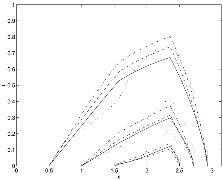
Figure 3: Contours of exact solution $u(x,t)$, —–, to compare with fourth-order numerical approximations (18): $\cdot\;\cdot\;\cdot\;\cdot$, the conventional approximation, errors $o(\alpha)$; $-\cdot-\cdot-$, the first correction, $o(\alpha^{2})$; and $-~{}-~{}-$ includes the second correction, $o(\alpha^{3})$. Burger’s equation (1) with parameters $\alpha=10$ and $\beta=0$ is discretised on $m=8$ intervals and drawn with contour interval $\Delta u=0.2$.

Table 2: Comparison of the errors $\varepsilon$, defined in (16), of the spatially fourth order model (18) for the first and third truncations in the nonlinear parameter $\alpha$ for various grid subintervals $m$. Observe that the higher order model is significantly less sensitive to the nonlinearity.

	$m=8$		$m=16$
$\alpha$	$o(\alpha)$	$o(\alpha^{3})$	$o(\alpha)$	$o(\alpha^{3})$
1	.0013	.0016	.0003	.0003
3	.0070	.0090	.0009	.0021
6	.0252	.0131	.0020	.0052
10	.0464	.0132	.0066	.0066
20	.0659	.0171	.0179	.0056
30	.0683	.0196	.0250	.0061

These fourth-order in space terms ensure a higher accuracy. Setting the artificial parameter $\gamma=1$ and truncating at various orders in $\|u\|$, equivalently in $\alpha$ because I set $\beta=0$ as before, we find that to see any appreciable difference between the nonlinearly higher-order models we have to increase the nonlinear parameter to $\alpha=10$ or more (from the $6$ used in the previous section). See in Figure 3 that the nonlinearly low-order approximation is a little in error, but that the higher-order models are generally better. They are reasonably accurate despite the large nonlinearity, $\alpha=10$, even though there is only $m=8$ intervals in one period. A more comprehensive summary of the numerical errors in given in Table 2 which compares the overall error $\varepsilon$ for $m=8$ and $m=16$ elements over one period for the nonlinearity parameter ranging over $1\leq\alpha\leq 30$. Once again observe that the conventional $o(\alpha)$ model has errors roughly proportional to $\alpha$, whereas the $o(\alpha^{3})$ model is much less sensitive. As the model is fourth-order in space the errors here are an order of magnitude smaller than those in Table 1 of the previous section. This confirms the effectiveness of this approach to developing finite difference models.

However, because of the subtleties in the analysis of the nonlinear terms, the equivalent partial differential equation of a derived finite difference model will not reduce to the original pde to the expected order in $h$. For example, here the equivalent pde of the model (18), with $\gamma=1$, is

$$\frac{\partial u}{\partial t}+\alpha u\frac{\partial u}{\partial x}=\frac{\partial^{2}u}{\partial x^{2}}-\beta u^{3}+\frac{h^{2}}{12}\left(-2\alpha u_{x}u_{xx}+\alpha^{2}uu_{x}^{2}\right)+{\cal O}\left(h^{4}\right)\,,$$ (19)

which apparently differs from the generalised Burger’s equation by ${\cal O}\left(h^{2}\right)$. But note that this equivalent differential equation is obtained as $h\to 0$ keeping $\|u\|$ fixed, whereas the centre manifold model (18) is derived for fixed $h$ as $\|u\|\to 0$ but taking full account of nonlinear dynamics within the domain. The numerical results presented here support my contention that this centre manifold approach better models the pde for finite $h$ and $\|u\|$.

5 Conclusion

Using centre manifold theory is a powerful new approach to deriving finite difference models of dynamical systems. Many details need to researched for a general application of the theory. However, this particular example application to a generalised Burger’s equation (1) shows many promising features.

By introducing artificial internal boundaries we apply centre manifold theory (§2). The internal boundaries divide the domain of interest into sub-domains that look very much like finite elements. The theory guarantees essential properties required for a low-dimensional model, though the need to evaluate the asymptotic expressions for $\gamma=1$ weakens this assurance. First, a model exists parameterized in any reasonable way we desire. Second, the model is approached exponentially quickly by the original dynamics, in a time of ${\cal O}\left(h^{2}\right)$ for Burger’s equation, but possibly much quicker for higher-order pdes. The same theorem also assures us that the numerical model shares the same stability as the original pde dynamics. Lastly, an approximation to the model may be found to any order in the nonlinearity, using computer algebra for example. The resultant finite difference models are independent of valid rearrangements of the governing pde. In effect this technique analyses the actual dynamics of the pde as a whole—this is a holistic approach. For example, I am not aware of any other discretisation method that develops cross terms between the nonlinearities, yet the presence of $\alpha\beta$ and $\alpha^{2}\beta$ terms in (14) suggests that they are essential for good finite difference models. Specific numerical simulations in §3 and §4 show that the finite difference models derived for Burger’s equation are indeed accurate.

Further research is needed to incorporate physical boundary conditions into the model. The extra analysis should be straightforward, but the level of detail would increase significantly as near the physical boundary we would lose the translational symmetry between the elements. Then the intriguing issue of initial conditions needs further work. Following [16, 7, 18] we note that to make accurate forecasts with the numerical models we need to provide initial values $u_{j}^{0}$ which are not the initial field $u_{0}(x)$ sampled at the collocation points $x_{j}$. Instead preliminary work shows that $u_{j}^{0}$ should be approximately the average of $u_{0}(x)$ over each element. Non-autonomous forcing of the pde will need projecting onto the finite difference grid in a similar manner. The analysis of other pdes in possibly higher-spatial dimensions would appear to hinge upon being able to solve the linear part of the pde over the elements subject to forcing from the coupling across the artificially introduced internal boundaries. This is potentially quite complicated, but the results of the simple problems here suggest that the analysis could be very worthwhile.

Appendix A Computer algebra develops the approximations

Just one of the virtues of this centre manifold approach to modelling is that it is systematic. This enables relatively straightforward computer programs to be written to find the centre manifold and the evolution thereon [20, e.g.]. I believe computer algebra will be increasingly used to support research by performing extensive routine algebraic manipulations. To ensure correctness and to provide a basis for further work it seems reasonable to include the computer algebra code.

For this problem the iterative algorithm is implemented by a computer algebra program written in reduce Although there are many details in the program, the correctness of the results are only determined by driving to zero (line 59) the residual of the governing differential equation, evaluated on line 48, to the error specified on line 46 and with the residual of the internal boundary condition computed on lines 50–53. The other details only affect the rate of convergence to the ultimate answer.

COMMENT Try holistic finite differences on a generalised Burgers
equation.  Consider ODEs of the form u_t - u_xx = f(u,u_x) for
strictly nonlinear f where for Burgers equation f \propto -u.u_x .
Discretise the problem by mathematically introducing insulating
boundaries at grid midpoints, and coupling them together via a
parameter \gamma so that the original C^2 holds at the midpoints when
\gamma=1.  Treat \gamma as a perturbation parameter.
The unknown u(x,t) field is then a function of u_j(t)=u(x_j,t), where
each u_j evolve according to du_j/dt=g_j .
Tony Roberts, 12 Sept 1998;
% improve printing
on div; off allfac; on revpri; factor gam,usz,h;
% make function of xi=(x-x_j)/h
depend xi,x;
let df(xi,x)=>1/h;
% parameterise with evolving u(j)
operator u; depend u,t;
let df(u(~k),t)=>sub(j=k,g);
% intx computes \int_{-1/2}^{+1/2} ... dxi
operator intx; linear intx;
let { intx(xi^~p,xi) => (1+(-1)^p)/(p+1)/2^(p+1)
    , intx(xi,xi) => 0
    , intx(1,xi) => 1 };
% solves v_xixi=RHS s.t. v(0)=0 and v_xi(+1/2)+v_xi(-1/2)=0
operator solv; linear solv;
let { solv(xi^~p,xi) => (xi^(p+2)/(p+2)-(1-(-1)^p)*xi/2^(p+2))/(p+1)
    , solv(xi,xi) => (xi^3-3*xi/4)/6
    , solv(1,xi) => (xi^2)/2 };
% linear solution in jth interval
% usz is used to measure the order of terms in u_j
v:=usz*u(j);
g:=0;
% iteration
% the BC is crafted s.t. gam^p kept gives (2p)th order in space
% by (1-gam)*delta(vp+v)h/2-gam*mu(vp-v)=0 recognising u_t=u_xx
let { gam^3=>0, usz^4=>0 } ;
repeat begin
   deq:=df(v,t)-df(v,x,2)+(a*v*df(v,x)+b*v^3);
   vp:=sub(j=j+1,v);
   dv:=sub(xi=-1/2,vp)-sub(xi=1/2,v);
   svd:=(h/2)*(sub(xi=-1/2,df(vp,x))+sub(xi=1/2,df(v,x)));
   bcp:=(1-gam)*( svd -df(svd,t)*h^2/12 +df(svd,t,2)*h^4/120
                  -df(svd,t,3)*h^6*17/20160 )   -gam*( dv );
   bcm:=sub(j=j-1,bcp);
   gd:=(-bcp+bcm)/h^2-intx(deq,xi);
   g:=g+gd/usz;
   v:=v+h^2*solv(deq+gd,xi)-xi*(bcm+bcp)/2;
   showtime;
end until (deq=0)and(bcp=0);
bcp:=sub(xi=-1/2,df(vp,x))-sub(xi=1/2,df(v,x)); % check other IBC
deq:=sub(xi=0,v)-usz*u(j); % check amplitude
end;

References

- [1] J. Carr. Applications of centre manifold theory, volume 35 of Applied Math Sci. Springer-Verlag, 1981.
- [2] J. Carr and R.G. Muncaster. The application of centre manifold theory to amplitude expansions. I. ordinary differential equations. J. Diff. Eqns., 50:260–279, 1983.
- [3] J. Carr and R.G. Muncaster. The application of centre manifold theory to amplitude expansions. II. infinite dimensional problems. J. Diff. Eqns, 50:280–288, 1983.
- [4] H.C. Chang. Onset of nonlinear waves on falling films. Phys. Fluids A, 1:1314–1327, 1989.
- [5] P. Constantin, C. Foias, B. Nicolaenko, and R. Temam. Integral manifolds and inertial manifolds for dissipative partial differential equations, volume 70 of Applied Mathematical Sciences. Springer-Verlag, 1989.
- [6] S.M. Cox and A.J. Roberts. Centre manifolds of forced dynamical systems. J. Austral. Math. Soc. B, 32:401–436, 1991.
- [7] S.M. Cox and A.J. Roberts. Initial conditions for models of dynamical systems. Physica D, 85:126–141, 1995.
- [8] E. Freire, E. Gamero, E. Ponce, and L.G. Franquelo. An algorithm for symbolic computation of center manifolds. In Symbolic and algebraic computation (Rome, 1988), volume 358 of Lecture Notes in Comput. Sci., pages 218–230. Springer, Berlin-New York, 1989.
- [9] J. Fujimura. Methods of centre manifold multiple scales in the theory of nonlinear stability for fluid motions. Proc Roy Soc Lond A, 434:719–733, 1991.
- [10] L.G. Margolin and D.A. Jones. An approximate inertial manifold for computing burgers equation. Physica D, 60:175–184, 1992.
- [11] G.N. Mercer and A.J. Roberts. A complete model of shear dispersion in pipes. Jap. J. Indust. Appl. Math., 11:499–521, 1994.
- [12] E. Meron and I. Procaccia. Theory of chaos in surface waves: The reduction from hydrodynamics to few-dimensional dynamics. Phys. Rev. Lett., 56:1323–1326, 1986.
- [13] I. Procaccia. Universal properties of dynamically complex systems:the organisation of chaos. Nature, 333:618–623, 1988. 16th June.
- [14] R.H. Rand and W.L. Keith. Normal form and center manifold calculations on macsyma. In R. Pavelle, editor, Applications of Computer Algebra. Kluwer Acad, 1985.
- [15] A.J. Roberts. The application of centre manifold theory to the evolution of systems which vary slowly in space. J. Austral. Math. Soc. B, 29:480–500, 1988.
- [16] A.J. Roberts. Appropriate initial conditions for asymptotic descriptions of the long term evolution of dynamical systems. J. Austral. Math. Soc. B, 31:48–75, 1989.
- [17] A.J. Roberts. Low-dimensional models of thin film fluid dynamics. Phys. Letts. A, 212:63–72, 1996.
- [18] A.J. Roberts. Computer algebra derives correct initial conditions for low-dimensional dynamical models. Submitted to Comput. Phys. Comm., June 1997.
- [19] A.J. Roberts. Low-dimensional modelling of dynamical systems. preprint, USQ, February 1997.
- [20] A.J. Roberts. Low-dimensional modelling of dynamics via computer algebra. Comput. Phys. Comm., 100:215–230, 1997.
- [21] A.J. Roberts. An accurate model of thin 2d fluid flows with inertia on curved surfaces. In P.A. Tyvand, editor, Free-surface flows with viscosity, volume 16 of Advances in Fluid Mechanics Series, chapter 3, pages 69–88. Comput Mech Pub, 1998.
- [22] J.C. Robinson. The asymptotic completeness of inertial manifolds. Nonlinearity, 9:1325–1340, 1996.
- [23] S. Rosencrans. Taylor dispersion in curved channels. SIAM J. Appl. Math., 57:1216–1241, 1997.
- [24] R. Temam. Inertial manifolds. Mathematical Intelligencer, 12:68–74, 1990.
- [25] A. Vanderbauwhede. Centre manifolds. Dynamics Reported, pages 89–169, 1989.
- [26] S.D. Watt and A.J. Roberts. The accurate dynamic modelling of contaminant dispersion in channels. SIAM J Appl Math, 55(4):1016–1038, 1995.