Computations of the Julia and Mandelbrot sets of the Riemann zeta function and observations of their properties are made. In the appendix section, a corollary of Voronin’s theorem is derived and a scale-invariant equation for the bounds in Goldbach conjecture is conjectured.

1 Introduction and Motivation

In this paper, we shall present a series of diagrams showing the Julia set of the Riemann zeta function and its related Mandelbrot set. This computation of the Julia and Mandelbrot sets of the Riemann zeta function may be, with reference to the existing literature, the first attempt ever made.

As we shall see, the Julia and Mandelbrot sets of the Riemann zeta function have unique features and are quite unlike those of any elementary functions.

We shall also point out, in the Appendix, two known observations of approximate self-similarity in Number Theory — in the images of Riemann zeta function itself, and in the problem of the Goldbach conjecture where a functional equation or scale-invariant equation for the ds in Goldbach conjecture is conjectured.

2 Properties of the Iterated Maps of the Riemann Zeta Function

Definition 1 (Iterated Maps of the Riemann zeta function)

Denote the iterated maps of the Riemann zeta function $\zeta(s)$ as $\,\zeta_{n}:\bf\sf C\,\mapsto\,\bf\sf C\;$ such that

$$\zeta_{n}:s\;\mapsto\;\underbrace{\zeta(\zeta(\cdots\zeta}_{n\mbox{\footnotesize-times}}(s)\cdots))$$ (1)

Definition 2 (Attractor and Repellor)

A fixed point $p$ of $f(x)$ is an attractor if $|f^{\prime}(p)|<1$, a repellor if $|f^{\prime}(p)|>1$.

Lemma 1 (An Asymptotic Property of $\zeta(s)$)

$$\log|\zeta(-|\sigma|)|=|\sigma|\log(|\sigma|\!+\!1)-|\sigma|(1\!+\!\log 2\pi)+O(\log|\sigma|)\quad(\sigma\in\bf\sf R)\;.$$ (2)

Proof

From the functional equation of the Riemann zeta function

$$\zeta(1\!-\!s)=2\;(2\pi)^{-s}\;\Gamma(s)\;\cos\left(\frac{\pi s}{2}\right)\;\zeta(s)\;,$$ (3)

we have

$$|\zeta(\sigma)|\leq|(2\pi)^{\sigma}\pi^{-1}\Gamma(1\!-\!\sigma)\zeta(1\!-\!\sigma)|$$

as $|\sin(\sigma\pi/2)|\leq 1$.

As $\sigma\to\infty$, $\zeta(\sigma)\to 1$ faster than $(1+\sigma^{-q})\to 1$ for any positive real $q$,

$$\zeta(1\!+\!|\sigma|) = 1+O(|\sigma|^{-q})\;,$$

$$\log(\zeta(1\!+\!|\sigma|) = O(|\sigma|^{-q})\;,$$

$$\log(\Gamma(1\!+\!|\sigma|)) = (1+|\sigma|)\log(1+|\sigma|)-(1+|\sigma|)+O(\log|\sigma|)$$

$$\qquad\mbox{ (by Stirling's formula) }.$$

Thus,

$$\log|\zeta(-|\sigma|)| = -|\sigma|\log(2\pi)+(1+|\sigma|)\log(1+|\sigma|)-(1+|\sigma|)+O(\log|\sigma|)$$

$$= |\sigma|\log(|\sigma|+1)-|\sigma|(1+\log 2\pi)+O(\log|\sigma|)\;.$$

    

Theorem 1 (Fixed Points of $\zeta_{n}$)

The Riemann zeta function $\zeta(s)$ has one attractor fixed point at

$$\sigma=\alpha=-0.2959050055752\ldots$$

but infinitely many repellor fixed points.

Proof

For $\sigma>0$, $y=\sigma$ intersects $y=\zeta(\sigma)$ at only one point, $\sigma=\alpha_{+}=1.833772\dots$. $\zeta(\alpha_{+})$ is thus a fixed point of $\zeta_{n}$. Since $|\zeta^{\prime}(\alpha_{+})|=1.3742\ldots>1$, the fixed point at $\sigma=\alpha_{+}$ is a repellor.

For $-1<\sigma<0$, $y=\sigma$ intersects $y=\zeta(\sigma)$ at $\sigma=\alpha=-0.2959050055752\ldots$. $\zeta(\alpha)$ is thus a fixed point of $\zeta_{n}$. Since $|\zeta^{\prime}(\alpha)|=0.51273\ldots<1$, the fixed point at $\sigma=\alpha$ is an attractor.

For $\sigma\leq-1$, $\zeta(2\sigma\!+\!1)=0$ at $\sigma\in\bf\sf Z^{-}$, and $\zeta(\sigma)$ oscillates with amplitude $\gg|\sigma|$ (by Lemma 1). Thus for $\sigma\leq-1$, $y=\sigma$ intersects $y=\zeta(\sigma)$ twice for the interval of every two zeros of $\zeta(\sigma)$, and $|\zeta^{\prime}(\sigma)|\gg 1$ for $\sigma$ in the neighbourhood of these intersections. $\zeta_{n}$ has thus infinitely many repellor fixed points for $\sigma\leq-1$.     

3 Julia set and Mandelbrot set of $\zeta(s)+a$ for $s,a\in\bf\sf C$

For the quadratic map $F(a,s)=s^{2}+a$ where $s,a\in\bf\sf C$, we have the following definitions.

Definition 3 (Julia set)

The Julia set $J$ of a map $F$ is the boundary of the domains of the attractors of the iteration of $F$.

For example, if $A_{1},\;A_{2}$ are attractors of the iteration of a map $F$, $D(A_{1}),\;D(A_{2})$ are the domains of the attractors respectively, and $\partial D(A_{1}),\;\partial D(A_{2})$ are the boundaries of the domains respectively, then the Julia set of $F$ is $J=\partial D(A_{1})=\partial D(A_{2})$.

Definition 4 (Mandelbrot set)

The Mandelbrot set $M$ of a map $F(a,s)$, for a chosen initial iteration value $s=s_{0}$, is the set of values of the complex parameter $a$ which, in the iteration of $F(a,s)$ with the chosen initial value $s_{0}$, does not lie in the domain of attraction of complex infinity.

$$M=\{a:a\in\bf\sf C,\lim_{n\to\infty}F_{n}(a,s_{0})\not\to\infty\}\;.$$ (4)

The Mandelbrot set is related to the Julia set in the following theorem.

Theorem 2 (The Julia-Fatou Theorem)

[1, p. 105]
The Julia set $J$ of a map $F(a,s)$ for the given value of $a$ is connected if and only if ${\displaystyle\lim_{n\to\infty}}F_{n}(a,0)\not\to\infty$, i.e. if and only if $a$ belongs to the Mandelbrot set $M$ of the map $F(a,s)$ for $s=0$.

Though the above definitions are for polynomials and are not the most general for non-polynomials, we shall choose to adopt these definitions here to study, for starters, a particular one-parameter family of the iterated maps of the Riemann zeta function, i.e., that of $F(a,s)=\zeta(s)+a$.

The Riemann zeta function $\zeta(s)$ has one attractor at fixed point $s=\alpha$ (by Theorem 1). It is not known if $\zeta(s)$ has any non-real fixed point, and this remains to be proved.

The Julia set of $\zeta(s)$ has been numerically computed with Mathematica with the algorithm downloadable from the Internet  at

http://www.damtp.cam.ac.uk/user/scw21/riemann/

The results are presented in Figures 1, 2, 3 and 4. This may be the very first computation of the Julia set of $\zeta(s)$ ever attempted.

$\mbox{\sf Im}(s)$

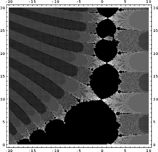
$\mbox{\sf Re}(s)$

Figure 1: The Julia set of $\zeta(s)$ for $-20\leq\mbox{\sf Re}(s)\leq 10\;\;$ and $\;\;0\leq\mbox{\sf Im}(s)\leq 30\,$.

The black region represents the basins of attraction of the attractor of the fixed point at $s=\alpha$ and those of attracting cycles. The other attractor is at $\infty$. The Julia set is the boundary of the black region.

The regions of different shades represent the various rates of amplitudes in iteration $\to\infty$, with the lighter shades having slower rates, and the darker shades, faster rates.

There is a reflection symmetry about the $\mbox{\sf Re}(s)$-axis due to the complex conjugate property of an analytic complex function.

$\mbox{\sf Im}(s)$

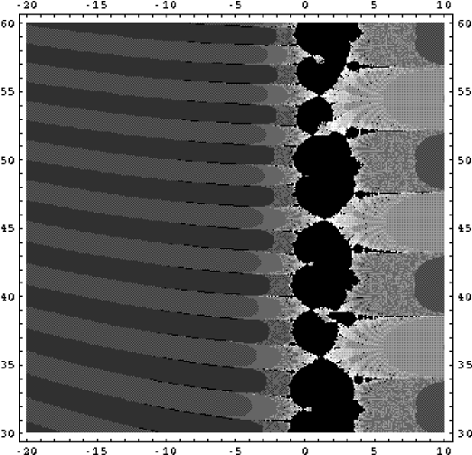
$\mbox{\sf Re}(s)$

Figure 2: The Julia set of $\zeta(s)$ for $-20\leq\mbox{\sf Re}(s)\leq 10\;\;$ and $\;\;30\leq\mbox{\sf Im}(s)\leq 60\,$.

Although a “piece” of the black region up along the $\mbox{\sf Im}(s)$-axis may resemble some other nearby “piece”, when examined in detail, each “piece”is unique and is distinct from any other “piece”.

$\mbox{\sf Im}(s)$

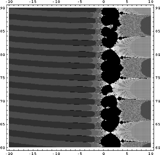
$\mbox{\sf Re}(s)$

Figure 3: The Julia set of $\zeta(s)$ for $-20\leq\mbox{\sf Re}(s)\leq 10\;\;$ and $\;\;60\leq\mbox{\sf Im}(s)\leq 90\,$.

The “pieces” of the black region seem to run indefinitely up the $\mbox{\sf Im}(s)$-axis and lies on $\mbox{\sf Re}(s)>0$ thereon.

$\mbox{\sf Im}(s)$

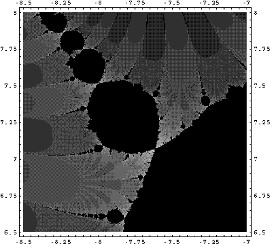
$\mbox{\sf Re}(s)$

Figure 4: Zooming in to reveal the self-similarity of the Julia set of $\zeta(s)$ for $-8.5\leq\mbox{\sf Re}(s)\leq-7\;\;$ and $\;\;6.5\leq\mbox{\sf Im}(s)\leq 8\,$.

We shall now turn to the Julia sets of $F(a,s)=\zeta(s)+a$ for $a\in\bf\sf C$. We shall evolve the Julia sets of $F(a,s)$ from one value of $a$ to another along a path in the complex plane of $a$, and study the dynamics in the change of the structure of the sets. In particular, we shall evolve the Julia sets of $F(a,s)$ along $a=0$ to $a=-1$ along the real axis of $a$ as in Figure 5, and similarly but in opposite direction from $a=0$ to $a=1$ along the real axis of $a$ as in Figure 6.

A numerical observation is that if sequence $F_{n}(a,s)$ in the Julia set iterations converges, then $F_{n}(a,s)$ tends to a fixed point which is a function $p_{J}(a)$ independent of $s$. This translates to the following conjecture:

Conjecture 1

Given a fixed $a$, $\zeta(s)+a=s$ has either one or no finite solution.

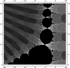
(i) $a=0$

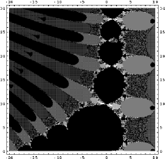
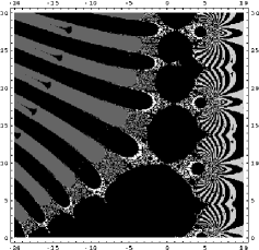
(ii) $a=-0.001$	(iii) $a=-0.01$
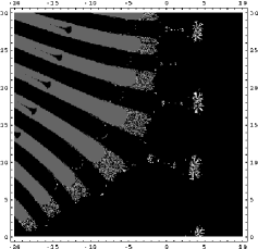
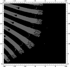
(iv) $a=-0.1$	(v) $a=-1$

Figure 5: Julia sets of $F(a,s)=\zeta(s)+a$

for $-20\leq\mbox{\sf Re}(s)\leq 10\,$, $0\leq\mbox{\sf Im}(s)\leq 30\,$, and

(i) $a=0$, (ii) $a=-0.001$, (iii) $a=-0.01$, (iv) $a=-0.1$, (v) $a=-1$.

The horizontal axis is $\mbox{\sf Re}(s)$, and the vertical axis is $\mbox{\sf Im}(s)$.

(i) $a=0$

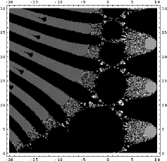
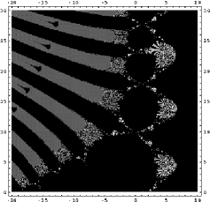
(ii) $a=0.001$	(iii) $a=0.01$
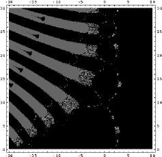
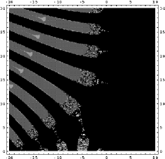
(iv) $a=0.1$	(v) $a=1$

Figure 6: Julia sets of $F(a,s)=\zeta(s)+a$

for $-20\leq\mbox{\sf Re}(s)\leq 10\,$, $0\leq\mbox{\sf Im}(s)\leq 30\,$, and

(i) $a=0$, (ii) $a=0.001$, (iii) $a=0.01$, (iv) $a=0.1$, (v) $a=1$.

The horizontal axis is $\mbox{\sf Re}(s)$, and the vertical axis is $\mbox{\sf Im}(s)$.

We shall now consider the Mandelbrot set of the Riemann zeta function. Given the map $F(a,s)=\zeta(s)+a$ for which the initial iteration value $s=s_{0}$ is a zero of the Riemann zeta function $\zeta(s)$, a value of the complex parameter $a$ belongs to the Mandelbrot set of $F$ if the iterated value $F_{n}(a,s_{0})$ does not tend to complex infinity in the limit the order of iteration, $n\to\infty$.

The results of the computation of the Mandelbrot set of $F(a,s)=\zeta(s)+a$ where the initial iteration value $s=s_{0}\in\{s:\zeta(s)=0$}, are presented in Figures 7, 8 and 9. This may also be the very first attempt at such computation.

However, the following about the Mandelbrot set of the Riemann zeta function was observed numerically and remains to be proved:

Conjecture 2

For the map $F(a,s)=\zeta(s)+a$, if $a$ belongs to the Mandelbrot set, then $F_{n}(a,s_{0})$ in the Mandelbrot iterations tends to a fixed point which is a function $p_{M}(a)$ independent of $s_{0}$, or tends to a $n$-cycle where $n\in\bf\sf Z^{+}$.

In addition, if Theorem 2 which applies to the quadratic map also applies to $F(a,s)=\zeta(s)+a$, from Figure 7, we can see that $a=0$ belongs to the Mandelbrot set of $F(a,s)=\zeta(s)+a$ for $s=0$, we deduce that the Julia set of $\zeta(s)$ is connected.

$\mbox{\sf Im}(s)$

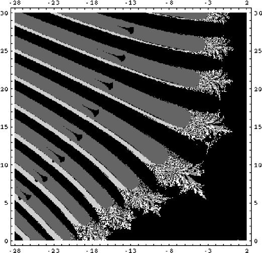
$\mbox{\sf Re}(s)$ for which $s$ is a zero of $\zeta(s)$, $-28\leq\mbox{\sf Re}(a)\leq 2\;\;$ and $\;\;0\leq\mbox{\sf Im}(a)\leq 30\,$.

Figure 7: Mandelbrot set of $F(a,s)=\zeta(s)+a$,

The black region represents the Mandelbrot set. The regions of different shades represent the various rates of amplitudes in iteration $\to\infty$, with the lighter shades having slower rates, and the darker shades, faster rates. There is a reflection symmetry about the $\mbox{\sf Re}(s)$-axis due to the complex conjugate property of an analytic complex function.

The overall picture has the feature of a “comb” or “bristles of a brush” with “hairy ends”. It is interesting to note that the “bristle” structures resemble those of the Julia sets for $|a|>>0$ in Figures 6  and 5  although the structures at the end of the “bristles” are different.

$\mbox{\sf Im}(s)$

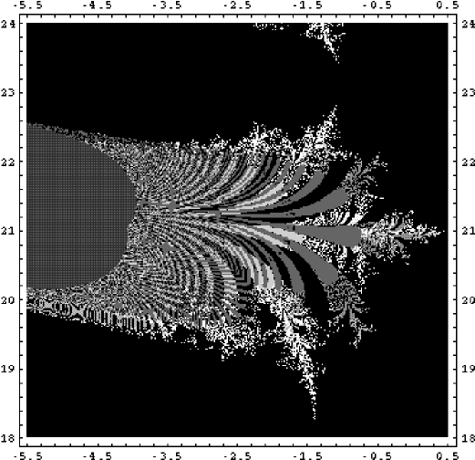
$\mbox{\sf Re}(s)$ of the Mandelbrot set of $F(a,s)=\zeta(s)+a$ for which $s$ is a zero of $\zeta(s)$, $-5.5\leq\mbox{\sf Re}(a)\leq 0.5\;\;$ and $\;\;18\leq\mbox{\sf Im}(a)\leq 24\,$.

Figure 8: Zooming in to reveal the self-similarity

The picture zooms onto the “hairy end” of a “bristle” only to reveal more “bristles” structures with “hairy ends” features, and ad infinitum.

$\mbox{\sf Im}(s)$

$\mbox{\sf Re}(s)$ $-28\leq\mbox{\sf Re}(a)\leq 2\;\;$ and $\;\;0\leq\mbox{\sf Im}(a)\leq 30\,$.

Figure 9: Mandelbrot set of $F(a,s)=\zeta(s)+a\;$ for $\;s=0$,

We can see that $a=0$ lies in the black region, and thus $a=0$ belongs to Mandelbrot set of $F(a,s)=\zeta(s)+a\;$ for $\;s=0$.

We shall consider the more general case, the iterations of fully-parametrized family of maps of the Riemann zeta function, in the next paper.

Appendix

Appendix A Examples of Approximate Self-Similarity and Scaling in Number Theory

A.1 Approximate self-similarity in the Riemann zeta function

We shall define approximate self-similarity and show that the following theorem due to Voronin implies that there are approximate self-similarity in the images of the Riemann zeta function.

Definition 5 (Approximate Self-Similarity to order $(\epsilon,r)$)

An n-dimensional map $f$ has approximate self-similarity to order $(\epsilon,r)$ when given $\epsilon>0$ and $r>0$, there exist $X_{a},X_{b}$ and $r_{b}$ such that $|f(X-X_{a})-f(r_{b}(X-X_{b}))|<\epsilon$ for all $|X|<r$, where $X=(x_{1},x_{2},\dots,x_{n})$.

Theorem 3 (Voronin)

[2] 
Let $0<r<1/4$ and let $f(s)$ be a complex function analytic and continuous for $|s|\leq r$. If $f(s)\neq 0$, then for every $\epsilon>0$, there exists a real number $T=T(\epsilon,f)$ such that

$$\max_{|s|\leq r}\big{|}f(s)-\zeta(s+3/4+iT)\big{|}<\epsilon\;.$$ (5)

Theorem 4

There exists approximate self-similarity to order $(\epsilon,r)$ for any given $\epsilon>0,\;0<r<1/4$ in the images of the Riemann zeta function.

Proof

Choose $f(s)=\zeta(\rho\,e^{i\theta}\!s+a)$ with fixed $\rho,\theta\in\bf\sf R$ and fixed $a\in\bf\sf C$ where $\rho>0,\;\theta\in[0,2\pi),\;0<|s|<1/4$, and choose $\epsilon$ to be arbitrarily small. The expression $\rho\,e^{i\theta}\!s+a$ with fixed $\rho,\theta,a$ describes a disc centred at $a$ with radius $\rho/4$ and orientation rotated at angle $\theta$.

By the inequality 5 in Theorem 3, we have self-similarities in the Riemann zeta function up to the order of $\epsilon$ between the images of the discs at different centres, scales and orientations (recentred by choosing a different fixed $a$, rescaled by choosing a different fixed $\rho$, and rotated by choosing a different fixed $\theta$), and the images of the discs along the upper half of the critical strip at $s+3/4+iT$ with different values of $T$.     

A.2 Scale-invariant equation for bounds in Goldbach conjecture

Conjecture 3 (Goldbach conjecture)

Every even integer $2n\geq 4$ can be written as a sum of two primes.

Definition 6

Define $G(2n)$ as the number of distinct decompositions of the even integer $2n$ into a sum of two primes ($3+5$ and $5+3$ are counted as identical decomposition).

Define $G_{L}(x)$ and $G_{U}(x)$ as the lower and upper monotonic bounding curves respectively of $G(2n)$ such that

$$\frac{dG_{L}(x)}{dx}>0\;\;\mbox{ and }\;\;\frac{dG_{U}(x)}{dx}\;\mbox{ for all }x\;,$$

and $G_{L}(2n)\leq G(2n)\leq G_{U}(2n)$ for all even integer $2n\geq 4$.

Thus, Goldbach conjecture states that $G_{L}(2n)\geq 1$ for all even integer $2n\geq 4$. However, the plots of $G(2n)$ in Figure 10 seem to show that the shapes of the bounding curves are invariant under scaling. This observation leads us to suggest a new conjecture:

$G(n)$
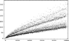
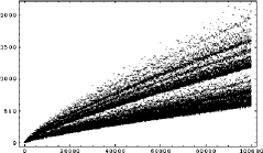
	$n$	$n$	$n$

Figure 10: Scale invariance in the bounding curves of $G(2n)$ and the approximate self-similar pattern in $G(2n)$

Conjecture 4 (Scale-invariant equation for bounds in Goldbach conjecture)

$G_{L}(x)$ satisfies the scale invariance equation

$$\quad\frac{G_{L}(ax)}{G_{L}(a)}\;=\;\frac{G_{L}(bx)}{G_{L}(b)}\quad(\mbox{for all real }\,a,b\neq 0)$$ (6)

$$\Rightarrow \frac{G_{L}(a)}{G_{L}(b)}\;G_{L}(bx/a)\;=\;G_{L}(x)\;,$$

and similarly for $G_{U}(x)$.

Although $f(ax)=f(a)\,f(x)\;$ (for all $a$) satisfies (6), the form of $G_{L}(x)$ is not in the form of $f(x)$. Since the simple power law $y(x)=\beta\,x^{\lambda},\;\beta,\lambda\in\bf\sf R$ is in the form of $f(x)$, we thus deduce that $G_{L}(x)$ is not a simple power law.

The patterns in $G(2n)$ as illustrated by Figures 11 and 12 are due to the distribution of prime numbers. Hardy and Littlewood [3] had derived an estimate for $G(2n)$ which accounts for the patterns,

$$G(2n)\sim\frac{2\,n\,C}{(\log n)^{2}}\prod_{p>2,\;p|n}\frac{p-1}{p-2}$$

where $p$ runs over all prime numbers, $p|n$ denotes that the product is taken only if $n$ is divisible by $p$, and $C$ is a constant,

$$C=\prod_{p>2}\left(1-\frac{1}{(p-1)^{2}}\right)=0.66016\dots\;.$$

$G(n)$

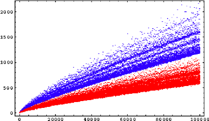
$n$

Figure 11: The subset of $\{G(2n)\}$ with $n$ being a multiple of $3$, $\{G(2(3n))\}$, is labelled by blue dots. The subset which is not, $\{G(2(3n+1))\}\cap\{G(2(3n+2))\}$, is labelled by red dots.

$G(n)$

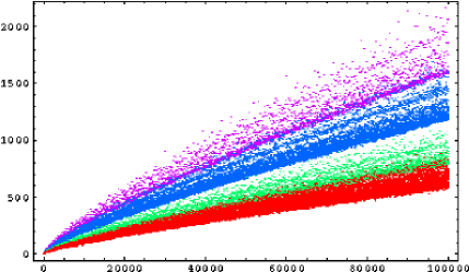
$n$

Figure 12: $\{G(2n)\;|\;n\equiv 0$ mod $3,\;n\equiv 0$ mod $5\}$ is labelled by magenta dots, $\{G(2n)\,|\,n\equiv 0$ mod $3,\;n\not\equiv 0$ mod $5\}$ by blue dots, $\{G(2n)\,|\,n\not\equiv 0$ mod $3,\;n\equiv 0$ mod $5\}$ by green dots, $\{G(2n)\,|\,n\not\equiv 0$ mod $3,\;n\not\equiv 0$ mod $5\}$ by red dots.

However, the scale-invariant property of the bounding curves $G_{L}(x)$ and $G_{U}(x)$ of $G(2n)$ as expressed in (6) is a new observation.

A.3 Open Problem

1. Derive the exact expressions for the bounding curves $G_{L}(x)$ and $G_{U}(x)$.

We shall attempt to derive $G_{L}(x)$ and $G_{U}(x)$ in the next paper.

Acknowledgement

Thanks to Michael Rubinstein, Keith Briggs and Gove Effinger for helpful comments.

References

- [1] P.G. Drazin, Nonlinear Systems, (Cambridge Univ. Press, Cambridge, 1992).
- [2] S.M. Voronin, “Theorem on the ‘Universality’ of the Riemann zeta-function”, Math. USSR Izvestija, 9(3) 443 (1975).
- [3] G.H. Hardy and J.E. Littlewood, “Some Problems of ’Partitio Numerorum’; III; On the Expression of a Number as a Sum of Primes”, Acta Math. 44, 1 (1922).