Testing for General Dynamical Stationarity with a Symbolic Data Compression Technique

Abstract

We construct a statistic and null test for examining the stationarity of time-series of discrete symbols: whether two data streams appear to originate from the same underlying unknown dynamical system, and if any difference is statistically significant. Using principles and computational techniques from the theory of data compression, the method intelligently accounts for the substantial serial correlation and nonlinearity found in realistic dynamical data, problems which bedevil naive methods. Symbolic methods are computationally efficient and robust to noise. We demonstrate the method on a number of realistic experimental datasets.

I Background

Symbolic methods have been used in the study of dynamical systems from the earliest days, most notably Kolmogorov and Sinai’s [1] use of metric entropy as a dynamical invariant, which spawned a significant mathematical industry in symbolic dynamics. Fraser [2] applied information theoretical concepts to construct useful algorithms and criteria for time-delay embeddings.

Stationarity, the notion that a system may be modeled well without time as an explicit parameter, is a prerequisite for the vast majority of nonlinear data analysis techniques. Only recently has there been some effort in constructing useful hypothesis tests suitable for realistic chaotic and nonlinear dynamical data.[3] In this work, we advocate a symbolic approach, on account of computational ease, and the connection to well-studied and powerful techniques of data compression heretofore rarely used in the physics literature which justify our statistical assumptions.

Comparing information in the symbolic dynamics observed from time series has a variety of uses besides stationarity tests [4, 5]. One that we mention here is a ’time-reversibility’ test: is the symbol stream statistically the same as its time-reversed version? This is important because Gaussian linear processes produce time-reversible time series, thus rejecting time-reversibility in an observed symbol stream implies that the data cannot be from that sort of process.

II The method

We have a series of symbols, either quantized from continuous-valued observations or directly measured, observed in discrete time: $s_{1},s_{2},s_{3},\ldots s_{N}$, each symbol from some alphabet $A$ re-expressed as integers $s\in\left\{1,2,\ldots,|A|\right\}$. In symbolic data analysis, the distribution of multi-symbol words provides information about time-dependent structure and correlation, just as, with continuous nonlinear data, time-delay embedding provides a vector space revealing dynamical information.

A first attempt at a stationarity test would be to apply the classical $\chi^{2}$-test to observed counts of distinct multi-symbol words observed in (say) the front and back halves of the data. Unfortunately, the assumption underlying this inference—that each datum is randomly and independently drawn from some distribution —is not true in realistic dynamical data. Short time correlations in physical data strongly couple symbols near in time; thus naive application of such tests fail miserably, usually towards spurious rejection. Indeed, dynamical dependence makes it difficult to construct a proper statistical null test for any hypothesis which allows chaotic or general nonlinear data in the null class, and few examples of this sort exist.

This work proposes a test procedure which quantifies whether two observed symbol streams have “the same dynamics” and its statistical significance, even in the presence of serial correlation and dependence. The algorithm is computationally rapid and does not require Monte Carlo simulation. There are two phases: construction of a symbolic predictive model, and the evaluation of a combination of classical statistics, this time on data constructed to be nearly independent.

A model based on an universal data compression algorithm factors out learnable dependence. Good compressors learn the conditional dependencies of symbols characteristic of the source process, thus less new information need be transmitted to reproduce the input data, assuming the decompresser can reconstruct the same model using the transmitted symbols. Fundamental results of information theory [6, 7] require that optimally compressed data are independent: this is the central theoretical justification for our subsequent application of classical statistical inference, and we feel one of the most useful concepts outside the specific application presented here.

Our model for the symbolic dynamics is a “context tree”: the recent symbols in the stream themselves define the state, known here as the context; contexts are analogous to the states reconstructed by time-delay embedding in conventional nonlinear dynamical analysis. Context tree modeling is a prominent contemporary development in the data compression field. We describe elsewhere [4, 5] other applications to nonlinear dynamics but in the present paper we specialize to stationarity testing.

The tree structure accumulates the statistics of observed symbol vectors down to maximum depth $d$, with distinct branches corresponding to distinct symbols of alphabet $A$ which occurred at prior times. The top node corresponds to no history, the first $|A|$ nodes a one-dimensional reconstruction of the most recent symbol, their $|A|^{2}$ descendents a 2-dimensional reconstruction of the two most recent and so forth. Naturally one only constructs the non-empty nodes.

Each node stores $|A|$ integers which record the distribution of every symbol $s_{t+1}$ that occurred immediately after its particular context $C$. From this information we can estimate the conditional probability for seeing the next symbol at every step: $\hat{P}(s_{t+1}|C)$. Observed data provides a data-based estimate of the emission, and thus, transition, probabilities.

In principle we can build a context tree to arbitrary depth: the most recently seen symbol can have a context that goes back to the start of the data stream. It is possible to construct such a tree efficiently (in time and space linear in the number of data [8]) but it is not useful to use the leaves directly to estimate conditional probabilities, since each leaf will have only one observation recorded. We need a balance between greater depth, which will reveal more structure, and larger numbers of observations at the nodes, which will give greater robustness against noise: the ubiquitous over-fitting issue. There are various methods of either selecting a specific subtree [9] or blending [10] different subtrees, all of which have varying compression properties. We use a state selection algorithm which is quite convenient for our stationarity test. We do not claim it is necessarily the state-of-the-art compressor, though its performance usually appears to be competitive on physical time-series data.

At each time step $t$, the time series history so far selects a set of possible contexts, or “excited nodes” of the tree, namely all nodes reachable by following branches which match the symbol history. We use an additional criterion to select from among the the excited nodes the “encoding node” at time $t$, which contains the estimated $\hat{P}(s_{t+1})$ to be employed. If one were literally compressing data, one would feed the successive estimated $\hat{P}$ for the actual symbols $s_{t+1}$ into an arithmetic coder, a well-studied algorithmic device [7] which generates the output bit stream with total code length at most two bits greater than $-\sum_{t}\log_{2}\hat{P}(s_{t+1})$. At a node with observed counts $c_{i}$, we use the Krichevsky-Trofimov [11] estimator,

$$\hat{P}(j)=(c_{j}+\frac{1}{2})/\sum_{i}(c_{i}+\frac{1}{2})$$

for symbol value $1\leq j\leq|A|$. $\hat{P}$ must be estimated before the new future symbol is included in the counts, because the decoder must be able to reconstruct the symbol statistics from previously processed input at every stage. There is no separate model or dictionary sending step. In our application, this is not essential and it is possible to envisage batch encoders, which differ in detail but not in principle from what we describe here.

Our method of encoding selects a specific encoding node for any symbol using a “predictive minimum description length (MDL)” principle due to Rissanen and later improved by others [9]. Each node stores a differential code length $\Delta=L_{p}-L_{s}$, the difference in code lengths which would have been emitted had the symbol been encoded using estimated distributions $\hat{P}$ at itself ($L_{s}$), or code length $L_{p}$ estimated using the parent’s counts. One descends the excited nodes from the top down, computing $\sum\Delta$, summing over all of the current node’s children’s value of $\Delta$. When this sum first becomes negative (assigning $\Delta=0$ to nonexistent child nodes) we have found the encoding node. The selection process has found the shortest matching context for which it would have been cheaper to have encoded past data using that context than longer matching contexts.

After encoding the current symbol, one updates $\Delta$ for each excited node:

$$\Delta\leftarrow\Delta+(-\log_{2}\hat{P}_{p}(s_{t+1})+\log_{2}\hat{P}_{s}(s_{t+1})),$$ (1)

the first expression using the node’s parent’s counts and the second using the node’s own counts. Note that $\Delta$ is a quantity maintained for each node independent of any previous choice of encoding node. Lastly, the conditional counts $c_{j}$ for all excited nodes are appropriately incremented with the new symbol, and new branches of the tree grafted for histories never seen before. It is important that the three phases be carried out in this particular sequence, repeating all three for each new symbol to encode.

Notice that, unlike fixed Markov modeling or the simplest version of time-delay embedding, the number of past symbols which contribute to predicting the future in a context tree is not uniform. Some past histories need to be deeply examined because there, long-past history influences the future significantly, whereas for other past histories, there is less need, either because future evolution is more unpredictable or there has been less information previously observed regarding those histories. In this respect, contexts are like “variable embeddings” [12].

III Stationarity test

After encoding all the symbols we carry out the stationarity test. The overall goal, answering the question “do two data sets appear to arise from the same underlying dynamical system”, translates to combining hypothesis tests performed at each encoding node regarding whether the encodings observed for both data sets (the distribution of future symbols actually encoded) could have come from a single underlying probability distribution $P(k)$, and if any apparent difference is statistically significant. At encoding contexts, we may use standard tests because these events ought to be nearly independent using a good compression algorithm. (A perfectly compressed data stream would be indistinguishable from a stream of independent random Bernoulli bits under any statistical test.)

At any node $n$, we have recorded the frequency with which symbol $k$ was encoded here, $e_{k;1}$ in the first set and $e_{k;2}$ in the second. (Note that $e_{k}\neq c_{k}$, the latter accumulating frequencies whenever a context was excited.) Assuming independence, the statistic

$$\chi^{2}=\sum_{k=1}^{|A|}\frac{\left(R^{1/2}e_{k;1}-R^{-1/2}e_{k;2}\right)^{2}}{e_{k;1}+e_{k;2}}$$ (2)

with $R=\sum e_{k;2}/\sum e_{k;1}$ follows the standard $\chi^{2}$ distribution with $|A|-1$ degrees of freedom under the null hypothesis that both empirical probability distributions came from the same underlying distribution[13]. Given the value of $\chi^{2}$ and the degrees of freedom, standard numerical algorithms provide a likelihood $L$ asymptotically uniform $L\in(0,1)$ under the null. Small values of $L$ reject the null at the given significance level, e.g. $\L<0.01$.

The asymptotic distribution of the $\chi^{2}$ test used in the computation of $L$ becomes increasingly inaccurate as the number of observations decreases. Thus for $\sum e_{k}<75$ (an arbitrary cutoff) we instead use a combinatorial test for differences in proportions, called Fisher’s exact test. As the test is much simpler in the $2\times 2$ case, we keep the observation for the most frequent symbol (bin $m$ which achieves $\max(e_{m;1}+e_{m;2})$) and merge the others into $e_{o;1},e_{o;2}$, resulting in four quantities conventionally expressed in a “contingency table”, with cumulative row and column sums:

$$\begin{array}[]{c|c|c}e_{m;1}&e_{o;1}&n_{1}\\ e_{m;2}&e_{o;2}&n_{2}\\ \hline\cr n_{m}&n_{o}&N\end{array}$$

Under the null that the difference in proportions between $m$ and $o$ counts is independent of being in set 1 and 2, the probability for seeing any particular table with the given marginal sums is:

$$p_{T}=n_{m}!n_{o}!n_{1}!n_{2}!/(e_{m;1}!e_{m;2}!e_{o;1}!e_{o;2}!N!).$$

One directly enumerates all tables with the given observed marginals (only a 1-d sum for a $2\times 2$ table) and sums $p_{T}$ for every table with a difference in proportions at least as great as that observed[14], resulting in a likelihood $L$ for accepting the null hypothesis at this node.

We combine these $M$ likelihoods, each measuring some aspect of of the same null hypothesis, into a single overall test. Under the null, the quantity

$$X^{2}=\sum_{k=1}^{M}-2\ln L_{k}$$ (3)

is $\chi^{2}$ distributed with $2M$ degrees of freedom, from which we compute our final ${\cal L}$, again uniform in $(0,1)$ under the null. Especially small values of ${\cal L}$ imply a small likelihood that this level of difference would have been observed had the two symbol datasets been generated by the same underlying dynamical process. This completes our desired test procedure.

IV Applications

We first test the accuracy of the null hypothesis. We produced an ensemble of 1000 time series from the $x$ coordinate of the “Lorenz 84” attractor: a tiny geophysical model with attractor dimension $d\approx 2.5$ [15]. Figure 2 shows the distribution of ${\cal L}$ comparing the first and second halves of each set, demonstrating ${\cal L}$ is close to uniform $\in(0,1)$. This is a stringent requirement and shows the success of our independence assumption, as it is difficult to get a high-quality null distribution with complicated arbitrarily correlated chaotic data in the null class. With this number of data, the test is also quite powerful.

We demonstrate discrimination power with a set of pressure data from an experimental model of a “fluidized bed reactor” [16]. This experimental system consists of a vertical cylindrical tube of granular particles excited from below by an externally input gaseous flow. In some parameter regimes (“slugging”), the particles exhibit complex motion which appears to be a combination of collective low-dimensional bulk dynamics and small-scale high-dimensional turbulence of the individual particles [16]. The observed variable was an azimuthally averaged pressure difference between two vertically separated taps. Figure 3 shows portions of time-delay embedding of orbits sections of the dataset taken at the same experimental parameters, and one when the flow was boosted by 5%. The change in the attractor is rather subtle and difficult to reliably diagnose by eye. Figure 4 shows the result of calculating ${\cal L}$ on a data set whose flow was increased at the midpoint. As the alphabet size increased and hypothesized breakpoint approached the true value of 50%, the strength of the rejection increased, ${\cal L}\rightarrow 0$. Even the binary alphabet case showed a significant rejection of the null. On data taken in stationary conditions ${\cal L}$ fluctuates randomly in $(0,1)$, as expected.

The Southern Oscillation Index, the normalized pressure difference between Tahiti and Darwin, is a proxy for the El Nino Southern Oscillation, as ocean temperature influences atmospheric dynamics. The period from mid 1990 to 1995 exhibited an anomalously sustained period of El Nino-like conditions (Fig. 5), perhaps indicative of global climate change. One statistical analysis [17] found such an anomaly quite unlikely assuming stationarity, but another group [18] used a different analysis and found it significantly more likely to be a chance fluctuation. Both papers used traditional linear forecasting models, with the difference centered around an auto-correlation based correction for serial correlation to arbitrarily reduce the degrees of freedom. We applied our algorithm to the 3-month moving average SOI (binary symbolized) testing the 5.4 year period in question against the rest of the series, with a resulting ${\cal L}\approx 0.01$, meaning that one would expect to see a region this anomalous by chance every 540 years. The result is closer to those of [18] than [17] but we certainly do not want to take any particular position regarding climate; rather, we wish to point out an application for our method where correcting for serial correlation automatically is useful.

Recent work has successfully used a distance in the symbolic space to fit unknown parameters of a physically motivated continuous model to observed data, including substantial observational and dynamic noise all in one framework, the situation where fitting models directly is difficult or unreliable. Tang et al [19] first proposed minimizing over free parameters the difference between an observed distribution of symbol words and that produced by discretizing some proposed model’s output. Daw et al [20] successfully used employed this technique to fit experimental internal combustion engine measurements to a low-dimensional dynamical model. The optimization target was a Euclidean norm in [19] and a chi-squared distance in [20]. On account of serial correlation, a true hypothesis test confirming or rejecting the apparent compatibility of observed data to best-fitting model was not possible in those works. We feel that our current method ought to provide a more intelligent and less ad hoc optimization goal, either by maximizing average ${\cal L}$ or perhaps minimizing the code length of the physical model’s output, encoded using the symbolic model learned from the observed data.

FIG. 1.: Example of a small context tree for a 3 symbol alphabet. The dotted node indicates that not all children necessarily exist, depending on the past symbols observed. Every node stores an estimated probability distribution, shown here for one node.

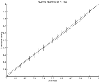
FIG. 2.: Quantile-quantile plot of ${\cal L}$ under the null hypothesis. The observed values of ${\cal L}$ are sorted and plotted vs their normalized index $(i+1)/1001$. Asymptotically the curve should approach the diagonal under the null. Bars are $\pm$ two standard deviations for 100 samples of 1000 uniform deviates $\in[0,1]$ processed similarly.

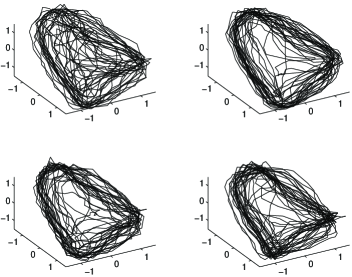
FIG. 3.: Phase space plots of the differential pressure signal from a fluidized bed reactor. Three are from the same parameters, one is different.

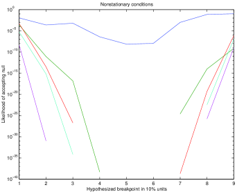
FIG. 4.: One fluidized bed system altered at the 50% mark, statistic ${\cal L}$ as a function of hypothesized breakpoint and symbolic alphabet precision. Curves for $|A|>2$ numerically underflowed to ${\cal L}=0$ toward the center and aren’t plotted. Null hypothesis emphatically rejected.

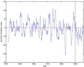
FIG. 5.: Three month moving average of the Southern Oscillation Index, the normalized pressure difference between Tahiti and Darwin, Australia. Strongly negative values correspond to El Nino events. Is the extended negative period from mid 1990 through 1995 especially anomalous?

REFERENCES

- [1] A.N. Kolmogorov, Dolk. Akan. Nauk. SSSR, 119 861–864 (1958); Y. Sinai, Dolk. Akad. Nauk. SSSR, 124, 768–771 (1959).
- [2] A. M. Fraser, IEEE Trans. Info. Theo., 35 245–262 (1989); A. M. Fraser and H. L. Swinney, Phys. Rev. A., 33 1134–1140 (1986).
- [3] M. B. Kennel, Phys. Rev. E 56 316 (1997); T. Schreiber, Phys. Rev. Lett., 78 843 (1997); A. Witt, J. Kurths, A. Pikovsky, Phys. Rev. E 58 1800 (1998).
- [4] L. Mason, A. I. Mees, K. Judd, “Context Trees and Embeddings”, Center for Applied Dynamics and Optimization, University of Western Australia (unpublished) (1997).
- [5] A. I. Mees, M. B. Kennel, “Symbolic Tree Embeddings and Nonlinear Dynamics”, in preparation, (1999).
- [6] C. E. Shannon, Bell Sys. Tech Journal 27 379 (1948)
- [7] T. Cover and J. Thomas, Elements of Information Theory (Wiley Interscience, New York, 1991).
- [8] F. M. Willems, IEEE Trans IT 44, 792 (1998).
- [9] J. Rissanen, IEEE Trans. Infor. Theory, 29 656–664 (1983); S. Bunton “A Percolating State Selector for Suffix-Tree Context Models” Proceedings Data Compression Conference 1997, 32–41, ed. J. A. Storer; M. Cohn, (IEEE Comput. Soc. Press, Los Alamitos, 1997)
- [10] F. M. Willems, Y. M. Shtarkov, and T. J. Tjalkens, IEEE Trans IT 41, 653 (1995).
- [11] Y. M. Shtarkov, T. J. Tjalkens, and F. M. J. Willems, Problems of Information Transmission, 33 17–28 (1997)
- [12] K. Judd, and A. I. Mees, Physica D, in press (1998).
- [13] The analytics degrade for small bin counts. For those bins, we merge any symbols whose expected count–for either set one or two–is less than five, reducing the degrees of freedom appropriately. If, after merging, there remain fewer than two symbols passing this criterion, then this node is wholly excluded.
- [14] In this discrete case, the sum will encounter tables exactly as likely as the observed one (such as the observed table itself); the summed for these tables is weighted by a uniform random deviate .
- [15] E. N. Lorenz, Tellus 36A, 98-110 (1984). The model is Each set was 5000 points long sampled every .
- [16] Daw C. S. et al, Phys. Rev. Lett. 75 2308–2311 (1995).
- [17] K. E. Trenberth and T. J. Hoar, Geophys. Res. Lett. 23 57–60 (1996)
- [18] D. E. Harrison and N. K. Larkin, Geophys. Res. Lett 24 1779–1782 (1997)
- [19] X. Z. Tang, E. R. Tracy, A. D. Boozer, A. deBrauw, and R. Brown, Phys. Rev. E 51, 3871 (1995).
- [20] C. S. Daw, M. B. Kennel, C. E. A. Finney, F. T. Connolly, Phys. Rev. E 57 2811 (1998).