Simulation of a Dripping Faucet

Abstract

A dripping faucet system is simulated. We numerically show that a hanging drop generally has many equilibrium shapes but only one among them is stable. By taking a stable equilibrium shape as an initial state, a simulation of dynamics is done, for which we present a new algorithm based on Lagrangian description. The shape of a drop falling from a faucet obtained by the present algorithm agrees quite well with experimental observations. Long-term behavior of the simulation can reproduce period-one, period-two, intermittent and chaotic oscillations widely observed in experiments. Possible routes to chaos are discussed.

Department of Physics, Tokyo Metropolitan University, Tokyo 192-0397
¹Department of Information Science, Kanagawa University, Kanagawa 259-1293

KEYWORDS: leaky faucet dynamics, computer simulation, drop formation, stability of hanging drops, chaos, bifurcation

§1 Introduction

The formation of drops is an intriguing phenomenon widely observed in everyday life. Although scientific researches on this subject date back to the seventeenth century[1], great progress has been achieved only recently, mainly in detailed studies on the behavior of drops near the breakup point. Breakup of a drop is a critical phenomenon corresponding to a singularity of a nonlinear partial differential equation obeyed by the fluid with free surface. Refined experiments to observe drops falling from nozzles for various viscosities provide much knowledge on this critical phenomenon[2, 3]. Eggers proposed a scaling theory which is universally applicable for axisymmetric drops with finite viscosity[4]. Numerical solutions of Navier-Stokes equations have been obtained with high precision for viscid[1, 5, 6] and inviscid[7] fluids, and well reproduce the observed shape of drops.

Another interesting aspect of the drop formation is the long-term behavior of a dripping faucet as a chaotic dynamical system. Since Shaw’s pioneering work[8] it has been confirmed in many experiments that dripping time intervals exhibit various types of periodic and chaotic oscillations including intermittency and hysteresis[9, 10, 11, 12]. Drastic change of an attractor is induced by a small variation of the flow rate, which is a main control parameter of the system. However, theoretical progress in this direction is not yet satisfactory. A simple “mass-on-a-spring” model has been proposed and an analog simulation of this model was reported to reproduce, in a qualitative sense, some experimental return maps[8, 9]. A numerical simulation based on a stochastic model was presented recently, in which an Ising-like system was used[13]. Since the latter model ignores kinetic terms, it might be applicable only for very small diameter of faucet( $\,\stackrel{{\scriptstyle\textstyle<}}{{\sim}}$ 0.5mm). In contrast, the mass-spring model corresponds to relatively large faucets, where the oscillation of the center of mass governs the basic dynamics. However, to explain the complex behavior observed in experiments systematically, information on the model parameters (for example, the spring constant) is essential, which is, unfortunately, not easily obtained. Both theoretical studies do not aim at investigating the realistic shape of drops, focusing on the long-term behavior of the dripping time intervals.

In our views, the reproduction of the shape of a drop is crucial in general understanding of the physics of the phenomenon. Indeed, our detailed simulation turns out to be successful in this respect. Even when one attempts to analyze the phenomenon using a simplified model, the knowledge of the drop shape is necessary for the correct choice of parameters. Our first goal is a long-term simulation using an algorithm which can also simulate the shape of drops reliably. After that, on the basis of detailed analysis of numerical data thus obtained, we are going to construct an improved mass-spring model which we expect reveals essential features of this complex system.

In this paper, we present a new algorithm for simulating a dripping faucet based on Lagrangian description instead of Eulerian one like Navier-Stokes equations. We decompose a drop into many parts (at most 300 $\sim$ 400 disks or less) and describe the dynamics in terms of time evolution equations obeyed by each part under the influence of gravity, surface tension and viscosity. After we observe that our algorithm can well reproduce shape of a drop at various stages of evolution, we proceed to a long-term simulation in which the growth and fission of a drop take place many times under a constant increase of the mass of the fluid. It will be shown that time series of the dripping time intervals reproduce various types of motions including period-one, period-two, intermittent oscillations etc. besides chaotic ones, as observed in many experiments. A bifurcation diagram will be presented which agrees well with a recent experiment.

In §2, we derive static shapes which are used as an initial condition for solving dynamical equations. In §3, equations of motion in Lagrangian description is presented. Computational results and experimental data are compared in §4. In Appendix A, we describe a variational algorithm to examine stability of static solutions. Our algorithm of simulation of dynamics is presented in Appendix B.

§2 Equilibrium States

We first derive static equilibrium shapes of a pendant drop where the gravitational and the surface tension forces balance each other. There is a maximum (i.e., critical) volume $V_{\rm c}$ for the stable state when the radius $a$ of the faucet is fixed. We will see below that there exist in general several equilibrium shapes when a volume smaller than $V_{\rm c}$ is given. As suggested by Padday and Pitt[14], only one among them is stable and realized, which we will show numerically.

The force balance equation of the drop is

$$P=\rho gz,$$ (1)

where $z$ is the vertical coordinate (the positive direction is defined to be downward), $P$ the pressure. The density $\rho$ is assumed to be constant throughout the fluid. The pressure (difference between the inside and the outside of the interface) is expressed in terms of the principal radii of curvature of the drop surface, $R_{1}$, $R_{2}$ as

$$P=\Gamma\left(\displaystyle\frac{1}{R_{1}}+\frac{1}{R_{2}}\right)\,,$$ (2)

where $\Gamma$ is the surface tension. Choosing the length, mass, and pressure units as

$$l_{0}\equiv\sqrt{\Gamma/\rho g}\,,\quad m_{0}\equiv\rho l_{0}^{3}\,,\quad P_{0}\equiv\sqrt{\rho g\Gamma}\,,$$ (3)

( $l_{0}=0.27$cm, $m_{0}=0.020$g and $P_{0}=$270dyn/cm² for water at 20 ^∘C,) we can set $g=\rho=\Gamma=1$.

For an axisymmetric drop, the radii of curvatures are given by

$$\displaystyle\frac{1}{R_{1}} = -\frac{{\rm d}\theta}{{\rm d}s}\,,$$ (4)

$$\frac{1}{R_{2}} = \frac{\cos\theta}{r}\,,$$ (5)

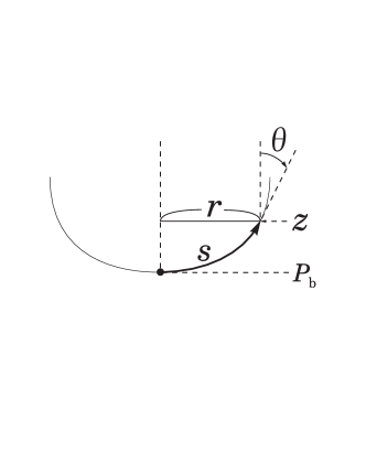
Fig. 1: Definition of variables.

where the variables $s$, $r$ and $\theta$ are defined in Fig. 1. The shape of the drop is thus obtained by integrating a set of ODE’s:

$$\left.\begin{array}[]{lll}\displaystyle\frac{{\rm d}r}{{\rm d}s}&=&\sin\theta,\\ &&\\ \displaystyle\frac{{\rm d}z}{{\rm d}s}&=&-\cos\theta,\\ &&\\ \displaystyle\frac{{\rm d}\theta}{{\rm d}s}&=&\displaystyle\frac{\cos\theta}{r}-z,\end{array}\right\}$$ (6)

with an ‘initial’ condition: $r(0)=0$, $z(0)=P_{\rm b}$, $\theta(0)=\pi/2$ at $s=0$, where $P_{\rm b}$ is the pressure at the bottom of the drop.

For a given value of $P_{\rm b}$, the solution of eq. (6) is unique. However, we need a boundary condition at the top of the drop to determine the upper limit of integration. Here it should be noted that eqs. (1) and (2) describe only the force balance, namely, they correspond to an equilibrium condition but not to any stability condition. We therefore have to select stable shapes out of the solutions of eq. (6). It is generally a difficult mathematical problem to examine whether an equilibrium state is stable or not when the system energy has not a lower limit, just like the present hanging drop. To the best of our knowledge, the existence of a stable shape and its uniqueness have not been proved. Padday and Pitt investigated stable shapes of drops under various conditions, assuming implicitly the uniqueness of the stable solution. In this paper, we numerically confirm that when there is one or more solutions of eq. (6), all except one are unstable. The rest is stable under any infinitesimal deformation, which we cannot prove but we conjecture.

§2.1 Drop hanging from a faucet

If we assume that the inner surface of the faucet is fully wetted and the outer surface is not wetted at all, the boundary condition is volume-radius limited[14]. That is, the shape of the drop is obtained by integrating the above equations up to $r=a$, where $a$ is the inner diameter of the faucet. Solution $r$ of eq. (6) oscillates as $s$ (and hence $z$) varies, which leads to, in general, many equilibrium shapes for fixed boundary condition. We can show, however, that at most one among them (the shortest shape) is stable.

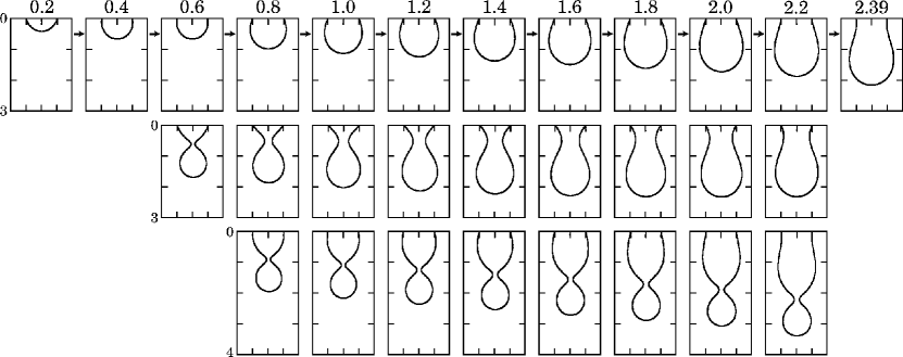
Fig. 2: Drop hanging from the faucet. $a=0.5$. Various equilibrium shapes for a fixed volume of the drop. Among them, only one (the top of each column) is stable. As the volume is increased, the shape changes as indicated by arrows. The maximum volume is $V=2.39$.

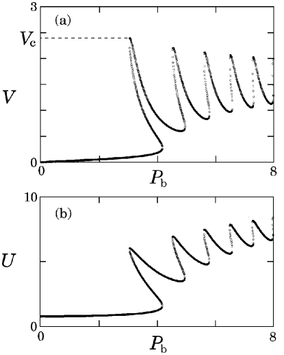
Fig. 3: Plot of the volume $V$ and the energy $U$ against the pressure at the bottom, $P_{\rm b}$ for a drop hanging from the faucet. $V_{\rm c}\approx 2.39$ is the critical volume. The radius of the faucet $a=0.5$.

In the following discussion, we fix at $a=0.5$. Figure 2 shows various profiles of drop obtained from eq. (6). The volume of drop, $V$ and its potential energy, $U$ are plotted against the bottom pressure, $P_{\rm b}$ in Figs. 3(a) and 3(b), respectively. The energy $U$ is the sum of the gravitational energy $U_{g}$ and the energy of surface tension $U_{\Gamma}$: $U=U_{g}+U_{\Gamma}$. These quantities are calculated from solutions of eq. (6). Figure 3(a) indicates that, as a function of $V$, $P_{\rm b}$ is generally multi-valued (when $V\begin{minipage}{12.0pt} \vspace{0pt}$\,\stackrel{{\scriptstyle\textstyle>}}{{\sim}}$\end{minipage}0.6$). For example, two possible profiles with the same volume $V=0.6$ (having $P_{\rm b}=3.86$ and 4.80,) are presented in the third column of Fig. 2. Also, one can see from Fig. 3(a) that there are many shapes with the same volume, say $V=1.5$. Each column of Fig. 2 presents several equilibrium profiles corresponding to a fixed volume. The drop on the top of each column has the lowest bottom pressure $P_{\rm b}$, and the second (third) one has the second (third) lowest $P_{\rm b}$. These profiles show that when the volume is fixed, the lower $P_{\rm b}$ corresponds to the shorter drop length (= the pressure difference between the top and the bottom of drop) as can easily be understood from eq. (2).

Observing Figs. 3(a) and 3(b) together, one can see that when the volume is fixed and if there are more than one equilibrium shapes (which takes place for $V\begin{minipage}{12.0pt} \vspace{0pt}$\,\stackrel{{\scriptstyle\textstyle>}}{{\sim}}$\end{minipage}0.6$), the shape with smaller $P_{\rm b}$, namely, a shorter shape, has a lower energy. This means that a decrease of the surface energy due to lowering $P_{\rm b}$ overwhelms an increase of the gravitational energy induced by lifting up the center of mass. The relation such that the lower $P_{\rm b}$ corresponds to the lower $U$ generally holds in volume-radius limited systems but not for volume-angle limited ones like a drop hanging from an infinite horizontal plane. (The volume-angle limited systems will be mentioned later on.) Now one might expect that the stable shape has the smallest equilibrium energy. But that is not self-evident. In fact, it turns out that the statement is true for the volume-radius limited system, but not for the volume-angle limited one. In order for any equilibrium shape to be realized, $U$ must increase under any infinitesimal deformation with the constraint such that both $V$ and $a$ are fixed.

In Appendix A, we derive a sufficient condition for stability. Stability of shapes that do not satisfy this sufficient condition are numerically examined and it was found that any equilibrium shape except the one having the lowest $P_{\rm b}$ (and hence the shortest one) is unstable under some axisymmetric deformation. That was examined for various values of the top radius $a$. On the other hand, it is difficult to determine whether or not the shortest shape, which has the lowest energy, is really stable under any infinitesimal deformation. We have studied several types of axisymmetric deformations and conjecture that the shortest shape is stable at least under any axisymmetric deformation, so that the profile on the top of each column is realized when the volume is given as indicated. The drop on the right end in the first row, having a neck close to the tip of the faucet, is also stable. Its volume $V=2.39$ is almost equal to the critical volume $V_{\rm c}$ indicated in Fig. 3(a). After all, as the volume increases, the profile of static drop changes from left to right in the first row of Fig. 2.

Interestingly, there are equilibrium shapes with infinite numbers of necks (for $V\approx 1.5$ when $a=0.5$), although such shapes are not realized because they are unstable under infinitesimal deformations.

§2.2 Drop hanging from an infinite horizontal plane

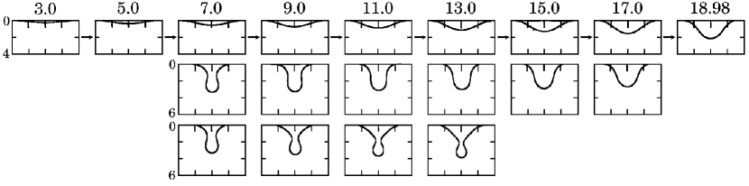
Fig. 4: Same as in Fig. 2  but for a drop hanging from the ceiling.

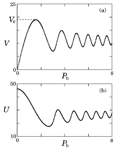
Fig. 5: Same as in Fig. 3  but for a drop hanging from the ceiling. The maximum volume is $V=18.98$.

Drops seen for example on the ceiling in the bath-room are volume-angle limited systems. They can also be obtained by integrating eq. (6) up to $\theta=\pi/2$ if the plane is fully wetted. Several equilibrium shapes with fixed volume are presented in Fig. 5. Plots of $V$ vs. $P_{\rm b}$ and $U$ vs $P_{\rm b}$ are given in Figs. 4(a) and 4(b), respectively. In each column of Fig. 5, profiles are arranged in increasing order of $P_{\rm b}$ (and hence increasing order of drop length). From a variational analysis, all profiles except the first row are found to be unstable under some axisymmetric deformation. As the volume increases, the realized static shape of drop changes from left to right in the top row.

It should be noted that if there are more than one equilibrium shapes, the stable one is the shortest but its energy is the second lowest as can be seen from Figs. 4(a) and 4(b). This is not surprising because the equilibrium state with the lowest energy is, as pointed out already, not necessarily stable for systems whose energy has not a lower bound. In the present case, each shape in the second top row of Fig. 5 has a lower energy than in the top row, which implies that a decrease of the gravitational energy overwhelms an increase of the surface energy. But the shape cannot be stable under some axisymmetric deformation.

The critical volume is $V_{\rm c}\approx 18.98(=0.37$cm³ for water at 20^∘ C). A drop larger than this volume cannot be suspended from the ceiling.

§3 Lagrangian Description of Fluid Motion

We take the following assumptions:

1. Incompressible fluid.

2. Axisymmetry.

3. Horizontal component of the fluid velocity can be neglected in comparison with vertical one.

4. Vertical component of the velocity depends only on the vertical coordinate.

5. No exchange between upper and lower parts of fluid.

Assumption (5) is derived from assumptions (3) and (4). These assumptions correspond to the shallow-water theory applied to axisymmetric systems[15] and have been used widely [16, 7, 1].

Let us denote the volume of the fluid below the vertical coordinate $z$ (the positive direction is defined to be downward) by

$$\xi(z,t)\equiv\int_{z}^{z_{\rm b}(t)}\pi r(\zeta,t)^{2}{\rm d}\zeta\,,$$ (1)

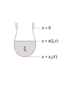
Fig. 6: Definition of variables.

where $z_{\rm b}(t)$ is the vertical coordinate of the bottom at time $t$ and $r(z,t)$ is the radius of the fluid at the coordinate $z$. Then, from assumptions (5), $\xi$ can be used as a Lagrangian variable. (See Fig. 6.)

The kinetic energy is thus given as

$$E_{\rm kin}=\displaystyle\frac{\rho}{2}\int_{0}^{\xi_{0}(t)}v^{2}{\rm d}\xi\,,$$ (2)

$$v\equiv v_{z}\equiv\frac{\partial z(\xi,t)}{\partial t}\,.$$

Here, the coordinate of the top of the drop ($=$ the end of the faucet) is defined as $z=0$, and $\xi_{0}(t)\equiv\xi(0,t)$ is the total volume of the drop. The gravitational energy is

$$U_{g}=-\rho g\int_{0}^{\xi_{0}(t)}z(\xi,t){\rm d}\xi\,.$$ (3)

The surface energy is expressed as

$$U_{\Gamma}=\Gamma\displaystyle\int_{0}^{z_{\rm b}(t)}2\pi r(z,t)\sqrt{1+\{\partial r(z,t)/\partial z\}^{2}}{\rm d}z\,,$$ (4)

which can be rewritten as

$$U_{\Gamma}=\Gamma\displaystyle\int_{0}^{\xi_{0}(t)}\sqrt{4\pi z^{\prime}+\frac{(z^{\prime\prime})^{2}}{(z^{\prime})^{4}}}{\rm d}\xi\,,$$ (5)

where

$$z^{\prime}\equiv\displaystyle\frac{\partial z(\xi,t)}{\partial\xi}\,,\hskip 28.45274ptz^{\prime\prime}\equiv\displaystyle\frac{\partial^{2}z(\xi,t)}{\partial\xi^{2}}\,.$$

Equations (2), (3) and (5) yield Lagrangian of the system as

$${\cal L}=E_{\rm kin}-U_{g}-U_{\Gamma}\,.$$ (6)

The effect of the viscosity is expressed by a dissipation function, $\dot{E}_{\rm kin}$ (namely, the time derivative of the Kinetic energy of fluid) as [15]

$$\begin{array}[]{lll}\dot{E}_{\rm kin}&=&-\displaystyle\frac{1}{2}\eta\int_{0}^{\xi_{0}(t)}\sum_{i,j}\left(\frac{\partial v_{j}}{\partial x_{i}}+\frac{\partial v_{i}}{\partial x_{j}}\right)^{2}{\rm d}\xi\\ &=&-3\eta\displaystyle\int_{0}^{\xi_{0}(t)}\left\{\frac{\partial v(z,t)}{\partial z}\right\}^{2}{\rm d}\xi\,.\end{array}$$ (7)

In the above, we have used the relation

$$\frac{\partial v_{x}}{\partial x}+\frac{\partial v_{y}}{\partial y}+\frac{\partial v_{z}}{\partial z}=0\,,$$

so that

$$\frac{\partial v_{x}}{\partial x}=\frac{\partial v_{y}}{\partial y}=-\frac{1}{2}\frac{\partial v_{z}}{\partial z}\,,$$

because of assumptions (1) and (2). Equation (7) reads

$$\dot{E}_{\rm kin}=-3\eta\displaystyle\int_{0}^{\xi_{0}(t)}\frac{\{\partial v(\xi,t)/\partial\xi\}^{2}}{\{\partial z(\xi,t)/\partial\xi\}^{2}}{\rm d}\xi\,.$$ (8)

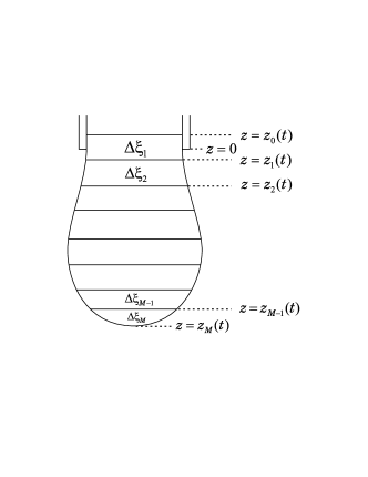
Fig. 7: Definition of variables.

We discretize the integral forms (2),(3),(5) and (8). Let the drop be sliced into $M$ disks by $(M-1)$ horizontal planes $z=z_{1},z_{2},\cdots z_{M-1}$ as Fig. 7. The volumes of these disks, $\Delta\xi_{j}$, are expressed as

$$\Delta\xi_{j}=\int_{z_{j-1}}^{z_{j}}\pi r(\zeta,t)^{2}{\rm d}\zeta;\quad\quad j=1,2,\cdots M;$$ (9)

$$z_{M}\equiv z_{\rm b}\,.$$ (10)

These volumes are conserved because of the incompressibility. (Variables at the top and the bottom of the fluid are defined suitably by taking account of the boundary condition. See below.) The mass of the disks are

$$\Delta m_{j}=\rho\Delta\xi_{j}\,,$$

which reads

$$\Delta m_{j}=\Delta\xi_{j}$$ (11)

by taking units such that $\rho=1$. Let the coordinate of the center of mass of the $j$-th disk be $\tilde{z}_{j}$. Then the kinetic and potential energies are given by

$$E_{\rm kin}\simeq\displaystyle\frac{1}{2}\sum_{j=1}^{M}\Delta m_{j}(\dot{\tilde{z}}_{j})^{2},$$ (12)

$$U_{g}\simeq-g\sum_{j=1}^{M}\Delta m_{j}\tilde{z}_{j}.$$ (13)

The dissipation function is

$$\dot{E}_{\rm kin}\simeq-3\eta\sum_{j=1}^{M}\displaystyle\frac{(v_{j}-v_{j-1})^{2}}{(z_{j}-z_{j-1})^{2}}\Delta m_{j},$$ (14)

where

$$v_{j}\equiv\dot{z_{j}}=\displaystyle\frac{\partial}{\partial t}z(\xi_{j},t).$$

The most important part of the algorithm is how to approximate the surface energy because the rigorous expression of the surface tension force includes higher-order derivatives in space coordinates. We approximate the surface energy $U_{\Gamma}=\Gamma S$ ($S$ is the surface area of the fluid) by patching many parts of conical surfaces: By defining the average radii of disks as

$$r_{j}=\displaystyle\sqrt{\frac{\Delta m_{j}}{\pi(z_{j}-z_{j-1})}}\,;\hskip 56.9055ptj=2,3,\cdots M\,;$$

the surface area in the interval $[(z_{j-1}+z_{j})/2,(z_{j}+z_{j+1})/2]$ is approximated as

$$S_{j} = \pi(r_{j}+r_{j+1})\sqrt{\displaystyle\frac{1}{4}(z_{j+1}+z_{j-1})^{2}+(r_{j}-r_{j+1})^{2}}$$ (15)

$${\equiv} S_{j}(z_{j-1},z_{j},z_{j+1})\,.$$

Then the surface energy becomes

$$U_{\Gamma}=\Gamma\sum_{j=1}^{M}S_{j}(z_{j-1},z_{j},z_{j+1})\,.$$ (16)

Further, using an approximation

$$\tilde{z}_{j}\simeq\displaystyle\frac{z_{j}+z_{j-1}}{2},\hskip 14.22636pt\hskip 14.22636pt\dot{\tilde{z}}_{j}\simeq\displaystyle\frac{\dot{z}_{j}+\dot{z}_{j-1}}{2}\,,$$ (17)

and substituting eq. (17) into (12) and (13), we obtain a Lagrangian of the discretized system as

$${\cal L}( z_{1} ,\cdots z_{M},\dot{z}_{1},\cdots\dot{z}_{M})$$

$$= {E_{\rm kin}}(\dot{z}_{1},\cdots\dot{z}_{M})-U_{g}(z_{1},\cdots z_{M})-U_{\Gamma}(z_{1},\cdots z_{M})\,.$$

(18)

Equations of motion in the Lagrangian description are thus obtained from

$$\frac{{\rm d}}{{\rm d}t}\frac{\partial{\cal L}}{\partial\dot{z}_{j}}=\frac{\partial{\cal L}}{\partial z_{j}}+\frac{1}{2}\frac{\partial\dot{E}_{kin}}{\partial\dot{z}_{j}}\,;\hskip 14.22636ptj=1,2,\cdots M.$$ (19)

In the present simulation, we used a further approximation

$$\tilde{z}_{j}\simeq z_{j},\hskip 28.45274pt\dot{\tilde{z}}_{j}\simeq\dot{z}_{j}$$ (20)

in place of eq. (17).

The top boundary is treated as follows: We mark a part of the fluid just inside the faucet and let its coordinate be $z_{0}(<0$ ). The volume in the interval $[z_{0},z_{1}]$ is

$$\Delta\xi_{1}=\int_{z_{0}}^{z_{1}}\pi r(\zeta,t)^{2}{\rm d}\zeta=\pi a^{2}|z_{0}|+\int_{0}^{z_{1}}\pi r(\zeta,t)^{2}{\rm d}\zeta\,,$$ (21)

which is constant as time passes. We fix the velocity of the fluid at the end of the faucet so that

$$\dot{z}_{0}=v_{0}\,;$$

namely, the volume of the fluid hanging from the faucet increases steadily with the constant flow rare $Q=\pi a^{2}v_{0}$. The volume of the first disk i.e., the volume in the interval [$0,z_{1}$], $\widetilde{\Delta\xi}_{1}$, increases as

$$\widetilde{\Delta\xi}_{1}=\int_{0}^{z_{1}}\pi r(\zeta,t)^{2}{\rm d}\zeta=\Delta\xi_{1}-\pi a^{2}|z_{0}|\,.$$

The coordinate $z_{1}(\geq 0$) increases according to the above relation. When $\widetilde{\Delta\xi}_{1}$ reaches a certain constant value, we redefine the numbers as

$$j+1\leftarrow j\,;\hskip 14.22636ptj=1,2,\cdots M\,;$$ (22)

and reset $z_{0}$ and $z_{1}$ to be

$$z_{0}\leftarrow-\Delta\xi_{1}/\pi a^{2},\quad\quad z_{1}\leftarrow 0\,.$$

In this way the number of disks $M$ increases by one. $M$ also increases when the relative thickness of any disk exceeds a certain limit and is divided in two. A more detailed description of the algorithm will be given in Appendix B.

§4 Results and Discussions

We choose $t_{0}\equiv(\Gamma/\rho g^{3})^{1/4}$ as the time unit. For water at 20 ^∘C, $t_{0}=0.017$ s. The unit of viscosity was chosen as $\eta_{0}\equiv(\rho\Gamma^{3}/g)^{1/4}$. Then viscosity is $\eta=0.002$ for water at 20 ^∘C. (Other units have been defined as eq. (3).) Setting values for the faucet radius $a$ and the velocity $v_{0}$, we simulate the time evolution of the dripping faucet.

§4.1 Comparison of shapes with experiments

Peregrine et al. observed details of the shapes of drops falling from a capillary tube[2]. We first see that the present algorithm can well reproduce their experimental data. The faucet radius was chosen to be $a=0.952$ corresponding 5.2 mm in diameter in their experiment. The flow rate of the water is not mentioned explicitly except their expression ’as slow as possible’. We chose as $v_{0}=0.01(=0.16$ cm/s). This is the velocity at the top of the drop (i.e., the tip of the faucet) employed as a boundary conditions. The breakup parameter is $\epsilon=10^{-4}$, which means when the minimum cross section of the necking region divided by the cross section of the faucet, $S_{\rm min}\equiv(r_{\rm min}/a)^{2}$, reaches this value we separate the drop from the remaining part and continue the simulation for the residue.

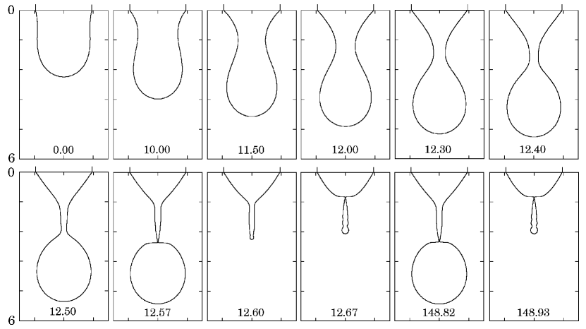
Fig. 8: Temporal change of the shape. $a=0.952$, $v_{0}=0.01$, $\eta=0.002$, $\epsilon=10^{-4}$. Initial condition: $P_{\rm b}=2.6$ corresponding to the initial volume $V_{\rm init}=4.77$.

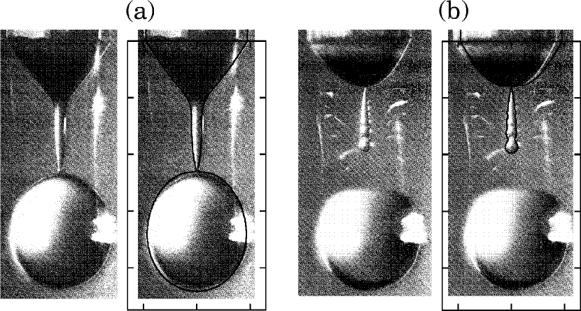
Fig. 9: A comparison of experimental and calculated drop shapes close to breakup moments. The photographs of the drops are from Peregrine et al. (J. Fluid Mech.,212 (1990) 25. Reprinted with permission of Cambridge University Press.) $a=0.952$, $v_{0}=0.01$, $\eta=0.002$, $\epsilon=10^{-4}$. (a) The moment at which $S_{\rm min}=5\epsilon$. (b) The moment at which $S_{\rm min}=\epsilon$.

In Fig. 8, we present profiles of drop falling from the faucet at various stages of evolution. The initial shape is taken from a static stable state of the volume $V_{\rm init}=4.77$, which has been obtained by integrating eq. (6) with $P_{\rm b}=2.6$. The time $t=12.57$ is the breakup moment, namely the moment at which $S_{\rm min}$ reaches $\epsilon$. The time $t=12.67$ is the second breakup moment. In Fig. 9, the profiles near the breakup moment are superimposed with the experimental photographs.

We see that the present simulation reproduces the observed shapes excellently. Especially, our shape of the satellite (the secondary small droplet) is closer to the observed one than that obtained from a different algorithm in which the viscosity is ignored.[7] (The shape at the first breakup moment has been well reproduced by Eggers[1].) If we remember several approximations made in our algorithm (particularly, eq. (20) and the procedure (12) in Appendix B), the agreement between simulation and experiment is amazingly good.

We can estimate an error of the breakup moment based on the following scaling relations[1, 6]:

$$r(t) \propto (t_{\rm c}-t)^{2/3}\quad{\rm for\quad inviscid\quad fluid}\,,$$ (1)

$$r(t) \propto (t_{\rm c}-t)^{1}\qquad{\rm for\quad viscid\quad fluid}\,,$$ (2)

where $t_{\rm c}$ is the critical point. The scaling region where eq. (2) holds is extremely small for water due to small viscosity (typical scales are $l_{\nu}\equiv\eta^{2}/\rho\Gamma\sim 1.4\times 10^{-6}$cm, $t_{\nu}\equiv\eta^{3}/\rho\Gamma^{2}\sim 1.9\times 10^{-10}$s). On the other hand, eq.(1) holds only approximately because of a crossover effect[6]. Nevertheless, these relations are useful enough to estimate the upper and lower limits of $t_{\rm c}$. Using eq. (1) and eq. (2) to extrapolate the plot of $r(t)$, we obtained , for example, $12.58<t_{\rm c}<12.66$ corresponding to the first breakup moment $t=12.57$.

§4.2 General feature of drops falling from a faucet

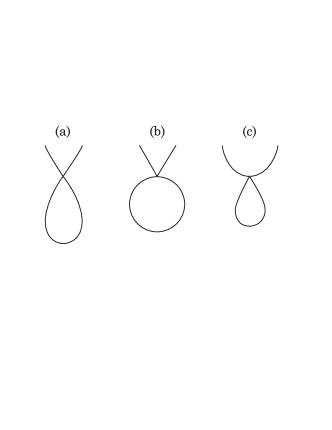
Fig. 10: The shape at the critical point is like (b) or (c) instead of (a). (c) is for pinching of a satellite.

As has already been recognized experimentally [2] and theoretically [7, 1], liquid drops do not have up-down symmetry like Fig. 10(a) near the critical point at which a drop separates. That is not due to the gravity. Instead, the symmetry spontaneously breaks down as sketched in Fig. 10(b) or (c) even without the gravitational effect. (The shape (c) corresponds to breakup of a satellite.) As we have seen, the marked asymmetry is observed in the present simulation as well. It should be noted that the asymmetry is a dynamical property of the fluid with free surface, therefore it cannot be predictable from the equilibrium shapes as in Fig. 2 and also not reproduced in the simulation neglecting kinetic terms[13].

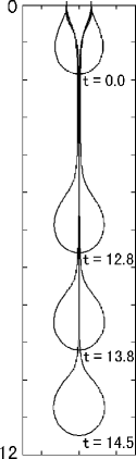
Fig. 11: Time evolution of a drop of glycerol. The length, time and viscosity units are $l_{0}=0.266$ cm, $t_{0}=0.0125$ s and $\eta_{0}=$4.26 g/cm s, respectively, corresponding to glycerol at 20 ^∘C.  $a=0.332$ (1.5 mm diameter), $\eta=3.50$, $v_{0}=0.05$.

Theoretically, from scaling properties derived by Eggers [4, 1], the asymmetric shapes near the critical point are expected to be universal irrespective of the viscosity, the faucet radius and the flow rate except the inviscid case. Practically however, it is also well known that the global shapes are strongly dependent on these conditions because the scaling law, even if it is exact, works only in the small region of time and space close to the critical point. In fact, the liquid bridge that connects the conical part (just below the faucet) and the spherical part shows a rough tendency to become long and thin for (1) large $\eta$, (2) large $a$ and (3) small $v_{0}$. These features are confirmed also in our simulation. For example, we present a simulation for large $\eta$. Figure 11 shows a temporal change of a drop of glycerol corresponding to an experiment by Shi et al [3]. Similar profiles have been obtained by solving the Navier-Stokes equations [5]. Both results well reproduce a long bridge observed in the experiment.

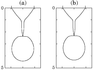
Fig. 12: Profile at the critical point in the limit of $v_{0}\rightarrow 0$. $a=0.952$, $\eta=0.002$, $\epsilon=10^{-4}$. (a) $v_{0}=0.01$. (b) $v_{0}=0$.

Strictly speaking, the length of the liquid bridge does not change monotonically with these parameters because of spatial and temporal oscillations of the liquid surface. The necking region is delicately affected by the interplay of these oscillations and liquid influx. Concerning the third condition (i.e., $v_{0}$-dependence), the shape tends to a final one in the limit of $v_{0}\rightarrow 0$ which should coincides with that obtained by setting $v_{0}=0$ and starting from an initial state with volume just above the critical value $V_{\rm c}$. For example, in case of parameter values ($\eta=0.002$, $a=0.952$, $v_{0}=0.01$, $\epsilon=10^{-4}$), with the initial volume $V_{\rm init}=4.77$, the first breakup occurred at the drop size $V_{\rm d}=3.85$ and the residue $V_{\rm r}=1.28$ (Fig. 12(a), which is the same profile at $t=12.57$ in Fig. 8). These results are to be compared with $V_{\rm d}=3.72$ and $V_{\rm r}=1.23$, which were obtained by a simulation with no flow: $v_{0}=0$, the same values for other parameters and the initial volume $V_{\rm init}=4.95$ slightly larger than the critical value (Fig. 12(b)). Two profiles look almost the same.

§4.3 Formation of secondary drop

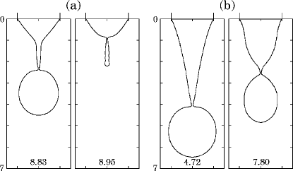
Fig. 13: Formation of the secondary drop. $a=1.0$, $\eta=0.002$, $\epsilon=10^{-3}$. Initial condition $P_{\rm b}=2.6$ corresponding to $V_{\rm init}=5.21$. Profiles are at the breakup moment, at which $S_{\rm min}=\epsilon$. The time of the breakup moment is written in each frame. (a) $v_{0}=0.003$. (b) $v_{0}=0.3$.

In the experiments focusing on long-term behavior of dripping faucets, the flow rate is usually chosen as a control parameter. As mentioned above, the shape of drop is strongly affected by the velocity $v_{0}$ or, equivalently, the flow rate. In Figs. 13(a) and 13(b), we present how the shape of drop at the second breakup moment depends on $v_{0}$. Parameters are chosen as ($a=1.0$, $\eta=0.002$, $\epsilon=10^{-3}$) commonly in (a) and (b); $v_{0}=0.003$ in (a) and $v_{0}=0.3$ in (b). The initial shape was commonly taken to be a static stable one. In both (a) and (b), two profiles describe the first and the second breakup moments (i.e., $S_{\rm min}=\epsilon$).

For smaller $v_{0}$, after the spherical drop detached from the bottom of the neck, a satellite droplet forms from the slender neck itself and separates from the conical part just below the faucet. The satellite is thus much smaller than the main drop. The volume ratio is 0.7 % in the present example. For larger $v_{0}$, the volume increases so rapidly that the slender liquid bridge disappears, the spherical part and the cone jointing directly. In the latter case, the secondary drop is again spherical and relatively large, its size being 44 % of the main drop. Results for the secondary-drop formation similar to Fig. 13 have been obtained from the simulation of inviscid fluid[7].

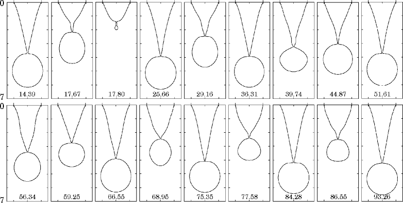
Fig. 14: Various shapes at each moment of breakup, at which $S_{\rm min}=\epsilon$. Continuation of Fig.13(b). $a=1.0$, $v_{0}=0.3$, $\epsilon=10^{-3}$.

Now a question is whether such successive processes, breakup of a main large drop followed by a smaller secondary drop can take place regularly or not. Details of shapes after the second breakup moment has not been reported so far. Figure 14 represents a continuation of Fig. 13(b), namely, a series of breakup moments for the same parameter values: $a=1.0,\;v_{0}=0.3$, where the first profile represents the third breakup moment. There appears sometimes a tiny droplet (smaller than $\sim 0.01$ % of the largest drops) splitting from the tip of the liquid cone just after the main drip, that is not presented here. Computational error may have led to such small droplets but the possibility that extremely small droplets really appear cannot be excluded. A larger drop and a smaller drop appear alternatively in Fig. 14, which looks almost periodic. Note, however, that large (small) drops are slightly different from each other in size and shape. These fluctuations are surely intrinsic, not due to computational error. A minute difference at each breakup moment can be an origin of not only fluctuations but also an irregular motion under certain conditions. Here we see that the dripping faucet is really a complex system.

§4.4 Long-term behavior

We present here results for $a=0.916$ corresponding to the faucet of 5mm in diameter used in a recent experiment by Katsuyama and Nagata[18]. For the long-term simulation, a larger value for the breakup parameter $\epsilon=4\times 10^{-3}$ was used to save the computational time. The velocity $v_{0}$ is chosen to be relatively small ($<0.16$), so that the secondary drop formation is like Fig. 13(a) instead of Fig. 13(b). In other words, pinching off of a satellite (or occasionally two successive satellites) smaller than 1 % of the largest drops always occurs just after breakup of a main drop. In the following analysis, we ignore these satellites. Then, the drop sizes distribute mostly in the range larger than 10 % of the largest drops.

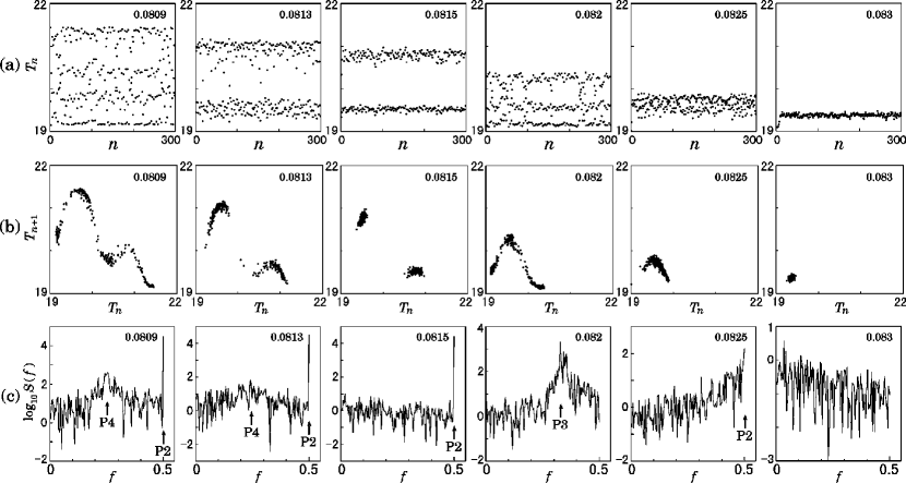
Fig. 15: (a) Plot of dripping time interval $T_{n}$ vs $n$ for various values of $v_{0}$. Value of $v_{0}$ is written in each frame. (b) Return map: plot of $T_{n+1}$ vs $T_{n}$. (c) Semi-log plot of power spectrum of (a) calculated from $2^{8}$ data points.

We let $T_{n}$ denote the $n$-th dripping interval, i.e., the time difference between the $(n+1)$-th and $n$-th drips. Neglect of satellites above mentioned implies that intervals $T_{n}$ which are smaller than $\sim 0.2$ are omitted, while $T_{n}$ for main drops are larger than $\sim 10$. Figure 15(a) represents plotting of $T_{n}$ vs $n$ for various values of $v_{0}$. Corresponding return maps, i.e., plots of $T_{n+1}$ vs $T_{n}$ and power spectra are given in Figs. 15 (b), and (c), respectively.

The time series data $\{T_{n}\}$ fluctuate considerably, but the power spectra can suggest types of bifurcation. As the control parameter $v_{0}$ is varied, period one (P1) motion at $v_{0}=0.083$ period-doubles $backward$ to period two (P2) motion. That can be confirmed from the power spectrum for $v_{0}$=0.0825 which exhibits a peak at frequency $f=1/2$, indicating P2 oscillation. When $v_{0}=0.082$, intermittent period three (P3) motion is observed, where the spectrum has a sharp peak at $f=1/3$. Another type of P2 motion is observed at $v_{0}=0.0815$. We found that the bifurcation to this type of P2 motion is $not$ period doubling from any P1 motion. Rather, forward and backward period doubling cascades to chaos, starting from this type of P2 motion, are expected. In fact, the spectra for $v_{0}=0.0813$ and 0.0809 exhibit a peak at $f=1/4$ besides a sharp peak at $f=1/2$, which indicates that the P2 motion at $v_{0}=0.0815$ period-doubles backward. The backward period doubling is widely observed also experimentally. Attractors in Fig. 15(b) closely resemble experimental ones.

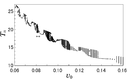
Fig. 16: Bifurcation diagram of the dripping interval $T_{n}$ vs $v_{0}$.

Figure 16 is a bifurcation diagram in which the parameter range of Fig. 15 is indicated. As suggested by Fig. 16, oscillations like those shown in Fig. 15 are quite typical in the present system, and repeatedly appear at different values of $v_{0}$. Similar types of oscillations are observed not only in the experiment by Katsuyama and Nagata for the same faucet size [18], but also in other experiments with smaller faucets[11, 12].

In the present simulation, at $v_{0}=0.074$ and $v_{0}=0.083$ for instance, the $T_{n}$ value is uniqe. In contrast, between these $v_{0}$ values (for $0.074<v_{0}<0.083$ for instance), the $T_{n}$ value is distributed over a finit range. This is seen on Fig. 16 in the form of a bloc, which repeats as $v_{0}$ increases. We may call this pattern a unit structure. Looking at Fig. 16 with reference to $T_{n}$, one sees each unit structure occurs periodically, namely, at the same interval in $T_{n}$. Qualitative agreement of our bifurcation diagram with the experiment by Katsuyama and Nagata is satisfactory in a wide range of the control parameter $v_{0}$, or equivalently the flow rate. In their bifurcation diagram, a unit structure similar to ours also appears repeatedly as the flow rate is varied.

§4.5 Further study

We have seen that the present simulation reproduces various aspects of the dripping faucet system which are observed experimentally. The next question is why the dripping faucet behaves like this. We will answer to this question in the forthcoming paper.[19] Here we give only an outline of it:

We construct an improved mass-spring model based on a detailed analysis of our numerical simulation. The model reveals the basic mechanism of the complex behavior of the dripping faucet system. A key of the new model is that the mass dependence of the spring-constant is taken into account. A similar global feature observed in the experiment and the simulation, i.e., the repeating unit structure in the bifurcation diagram, is reproduced also in the improved mass-spring model. This simplified model shows that each unit in the bifurcation diagram includes ordinary period doubling cascade to chaos, forward and backward period doubling cascade starting from P2 motion, intermittency and hysteresis. It is also clarified that the unit structure can be explained in terms of oscillations of the center of mass of the fluid, in other words, each unit is characterized by an integer which relates to the frequency of the oscillations during the time between two successive breakup moments.

Appendix A Stability Analysis

We consider an axisymmetric deformation such that the part between the interval $[z,z+{\rm d}z]$ is mapped onto the interval $[Z,Z+{\rm d}Z]$, where

$${\rm d}Z=\left[1+\epsilon(z)\right]{\rm d}z$$

with the constraint

$$\epsilon(0)=\epsilon(z_{\rm b})=0\,.$$ (3)

The coordinates at the top and the bottom of the drop are defined as $z=0$ and $z_{\rm b}$, respectively, which are mapped onto $Z=0$ and $Z_{\rm b}$ by the deformation.

Because the volume of each part is conserved before and after the deformation, the radius $r(z)$ is transformed as

$$R(Z)=\frac{r(z)}{\sqrt{1+\epsilon(z)}}\,.$$

The increment of the surface energy $U_{\Gamma}$ caused by the deformation is expressed as

$$\delta U_{\Gamma} \equiv 2\pi\Gamma\int_{0}^{Z_{\rm b}}R\sqrt{1+(R^{\prime})^{2}}{\rm d}Z$$

$${}-2\pi\Gamma\int_{0}^{z_{\rm b}}r\sqrt{1+(r^{\prime})^{2}}{\rm d}z$$

$$= \delta U_{\Gamma,1}+\delta U_{\Gamma,2}\,,$$

where $\delta U_{\Gamma,1}=O(\epsilon)$ and $\delta U_{\Gamma,2}=O(\epsilon^{2})$ are the first and the second order quantities of the small deformation $\epsilon$. The increment of the gravitational energy $U_{g}$ is

$$\delta U_{g}\equiv-\rho g\int_{0}^{Z_{\rm b}}\pi R^{2}Z{\rm d}Z+\rho g\int_{0}^{z_{\rm b}}\pi r^{2}z{\rm d}z=\delta U_{g,1};$$

$\delta U_{g}$ includes only linear terms of $\epsilon$, namely the second order term vanishes: $\delta U_{g,2}=0$. It is a little tedious but not difficult to derive the force-balance equation (1) and (2) from the equilibrium condition

$$\delta U_{\Gamma,1}+\delta U_{g,1}=0.$$

The stability condition is

$$\delta U_{\Gamma,2}>0,$$

where

$$\delta U_{\Gamma,2} = \frac{\pi\Gamma}{4}\int_{0}^{z_{\rm b}}\left[\phi(z)\epsilon^{2}+\psi(z)(\epsilon^{\prime})^{2}\right]{\rm d}z\,,$$ (4)

$$\phi(z) \equiv \frac{r}{\left(1+(r^{\prime})^{2}\right)^{5/2}}$$

$${}\times\left[-1+(r^{\prime})^{2}+(r^{\prime})^{4}-rr^{\prime\prime}\left(7-2(r^{\prime})^{2}\right)\right]\,,$$

(5)

$$\psi(z) \equiv \frac{r^{3}}{\left(1+(r^{\prime})^{2}\right)^{3/2}}\,.$$ (6)

The second term in the integrand is positive definite. Therefore the condition

$$\phi(z)>0\quad{\rm for}\quad 0<z<z_{\rm b}$$ (7)

is sufficient for the stability of equilibrium shape under any axisymmetric deformation $\epsilon(z)$.

When the drop has a neck, the condition (7) is not satisfied because $\phi(z)$ is negative at the neck ($r^{\prime}=0$, $r^{\prime\prime}>0$). We have found that all shapes with volume $V\begin{minipage}{12.0pt} \vspace{0pt}$\,\stackrel{{\scriptstyle\textstyle>}}{{\sim}}$\end{minipage}1.3$ in Fig. 2 and $V\begin{minipage}{12.0pt} \vspace{0pt}$\,\stackrel{{\scriptstyle\textstyle>}}{{\sim}}$\end{minipage}17.0$ in Fig. 5 violate this sufficient condition. (Some of them have no neck but do not satisfy (7).) However, such shapes are not necessarily unstable because the the homogeneous deformation $\epsilon^{\prime}=0$ is impossible under the constraint of eq. (3), and hence the second term of the integrant in eq. (A) always works in the direction of stabilization.

Therefore we first calculate $\phi(z)$ and if $\phi(z)<0$ in an interval $0\leq z_{1}<z<z_{1}+d$, the following infinitesimal deformation is considered:

$$\epsilon(z) = 2\Delta\frac{(z-z_{2})}{(\alpha d)^{2}\beta}\quad$$ (8)

$$\hskip 28.45274pt{\rm for}\quad z_{2}\leq z\leq\beta\alpha d+z_{2},$$

$$\epsilon(z) = 2\Delta\frac{(\alpha d+z_{2}-z)}{(\alpha d)^{2}(1-\beta)}\quad$$ (9)

$$\hskip 28.45274pt{\rm for}\quad\beta\alpha d+z_{2}\leq z\leq\alpha d+z_{2},$$

$$\epsilon(z) = 0\quad{\rm otherwise},$$ (10)

which leads to a stretch of the original shape by the length

$$\int_{z_{2}}^{z_{2}+\alpha d}\epsilon{\rm d}z=\Delta\,.$$

The parameters $z_{2}$ (satisfying $0\leq z_{2}<z_{2}+\alpha d<z_{\rm b}$), $\alpha$ ($>0$), and $\beta$ ($>0$) characterizing the deformation are varied and we examined if $\delta U_{\Gamma,2}/\Delta^{2}$ becomes negative. In this way, for fixed values of $V$ and $a$, all the equilibrium shapes except the shortest one, which has the lowest energy, are found to be unstable for the volume-radius limited systems. Also for the volume-angle limited systems, all the equilibrium shapes except the shortest one, which has the second lowest energy, are found to be unstable. All the shapes (including the largest one) on the top of each column in Figs. 2 and 5 are found to be stable at least under axisymmetric deformations.

Appendix B Algorithm

We employed a fourth-order Runge-Kutta method with adaptive stepsize control[17]. When the radius $a$ of the faucet and the velocity $v_{0}$ of liquid at the tip of the faucet are given, the simulation is done based on the following algorithm.

1. Initial shape
   We choose one of the stable equilibrium shapes obtained from the method described in §2.

2. Decomposition of a drop
   The drop of (1) is sliced with horizontal planes so that the drop is decomposed into many disks. The thickness of disks are such that the length $s$ of each disk measured along the edge of the section shown in Fig. 7 is equal. Therefore the disks near the bottom are relatively thin(see Fig. 7). The total number of the disks is denoted as $M$.

3. Coordinates and volumes of disks
   Vertical coordinates of the slice plane are denoted as $z_{1},\;z_{2},\;\cdots z_{M-1}$. They satisfy the relation

   $$0\leq z_{1}<z_{2}<\cdots<z_{M}\equiv z_{\rm b}\,,$$ (11)

   where

   $$z_{1}(t=0)=0\,.$$

   Further, we set $z_{0}$ to be a negative constant value: $z_{0}=z_{0}(t=0)<0$. The volume of the disk in the interval $[z_{j-1},z_{j}]$ are denoted as $\Delta\xi_{j}(j=1,2,\cdots M)$ and the volume in the interval $[0,z_{1}]$ as $\widetilde{\Delta\xi}_{1}$. These volumes are calculated precisely from the static solution employed as an initial condition.

4. Average radius of disks
   We define the average radii of disks as follows:

   $$\left.\begin{array}[]{llll}r_{j}&=&\sqrt{\displaystyle\frac{\Delta\xi_{j}}{\pi(z_{j}-z_{j-1})}}&\equiv\quad r_{j}(z_{j},z_{j-1})\,;\\ &&&j=2,3,\cdots M\,;\\ r_{1}&=&\sqrt{\displaystyle\frac{\widetilde{\Delta\xi}_{1}}{\pi z_{1}}}\,.&\hskip 5.69046pt(z_{1}>0)\end{array}\right\}$$ (15)

   (16)

5. Initial velocities of disks
   We set as $v_{j}(t=0)=v_{0}$ ($j=1,2,\cdots v_{M}$).

6. Tentative stepsize
   At $t=0$, we tentatively set as $\Delta t=\widetilde{\Delta t}$.

7. Adaptive stepsize
   From the time-evolution equations

   $$\left.\begin{array}[]{lll}\dot{z}_{j}&=&v_{j}\,,\\ \dot{v}_{j}&=&f_{j}(\{z_{i}\},\{r_{i}(z_{i},z_{i-1})\},\{v_{i}\})\,;\\ &&\hskip 14.22636ptj=1,2,\cdots M\,;\end{array}\right\}$$ (20)

   (21)

   we estimate the error $\widetilde{\Delta}$ for one step of fourth-order Runge-Kutta algorithm. Then $\widetilde{\Delta}$ is compared with our desired accuracy $\Delta_{0}$ and an adjusted stepsize $\Delta t$ is decided. This procedure is applied for all errors of variables $\{z_{i}\},\{v_{i}\}$ and the smallest value of $\Delta t$ is taken [17].

8. Time evolution
   Equation (21) is integrated by one time step i.e., from $t$ to $t+\Delta t$ using the fourth-order Runge-Kutta method.

9. Renewal of the stepsize
   From (8), we estimate the error $\widetilde{\Delta}$ in a similar way to (7) and renew the adapted stepsize $\Delta t$ for the next step.

10. Check of overtaking
    Because of assumption (5) in §4, any disk must not overtake the neighboring one, in other words, the relation (11) should be maintained all times. So if the condition of eq. (11) is violated, we choose a smaller value for $\Delta t$ and redo the same procedure (8). This does not occur if the accuracy $\Delta_{0}$ has been chosen small enough.

11. Increment of the number of disks
    When the volume of the first disk, $\widetilde{\Delta\xi}_{1}$ becomes larger than a certain constant value, we redefine variables as

    $$\begin{array}[]{lll}z_{j+1}&\leftarrow&z_{j}\,;\quad j=1,2,\cdots M\,;\\ v_{j+1}&\leftarrow&v_{j}\,;\quad j=0,1,\cdots M\,;\\ z_{1}&\leftarrow&0\,,\end{array}$$

    and reset $z_{0}$ to be the initial value $z_{0}(t=0)$. In this way, $M$ increases by one.

12. Division of a disk
    If the ratio of the width to the radius, $(z_{j}-z_{j-1})/r_{j}$ is over a certain limit for any disk, the disk is divided into two parts so as to conserve both the total volume and the momentum. In this way, $M$ is increased by one. It should be noted that the way of division is not unique. On the other hand, it turns out that there is no solution of division under additional constraint such that the energy is rigorously conserved. We divided disks in such a way that the spatial derivatives of velocity is conserved besides the volume and the momentum.

13. Coalescence of disks
    When the radii of some neighboring disks become larger than a certain value, the two disks are combined into one. Then $M$ decreases by one.

14. Renewal of disk radii
    From the renewed values of $\{z_{i}\}$ and $\{\Delta\xi_{i}\}$, the values of $\{r_{i}\}$ are replaced using eq. (16).

15. Breakup of the drop
    When the shape of the drop has a neck (or necks), the minimum radius $r_{\rm min}$ in the necking region is compared with the faucet radius. If its relative cross section $S_{\rm min}\equiv(r_{m}/a)^{2}$ is less than a critical value, then the part below the neck is separated. After that, the number of disks becomes $M\leftarrow(m-1)$ where $m$ is the disk number corresponding to $r_{m}=r_{\rm min}$.

16. Return to (8)
    We go back to the procedure (8) and continue the iterations.

References

- [1] J. Eggers: Rev. Mod. Phys. 69 (1997) 865.
- [2] D. H. Peregrine, G. Shoker and A. Symon: J. Fluid Mech. 212 (1990) 25.
- [3] X. D. Shi, M. P. Brenner and S. R. Nagel: Science 265 (1994) 219.
- [4] J. Eggers: Phys. Rev. Lett. 71 (1993) 3458.
- [5] J. Eggers and T. F. Dupont: J. Fluid Mech. 262 (1994) 205.
- [6] J. Eggers: preprint “Singularities in droplet pinching without viscosity” (chao-dyn/9705005, 1997).
- [7] R.M.S.M. Schulkes: J. Fluid Mech. 278 (1994) 83.
- [8] R. Shaw: The Dripping Faucet as a Model Chaotic System (Aerial Press, Santa Cruz, 1984).
- [9] P. Martien, S. C. Pope, P. L. Scott and R. S. Shaw: Phys. Lett. 110A (1985) 399.
- [10] X. Wu and A. Schellyt: Physica 40D (1989) 433.
- [11] K. Dreyer and F. R. Hickey: Am. J. Phys. 59 (1991) 619.
- [12] J. C. Sartorelli, W. M. Goncalves and R. D. Pinto: Phys. Rev. E 49 (1994) 3963.
- [13] P. M. C. de Oliveira and T. J. P. Penna: J. Stat. Phys. 73 (1993) 789.
- [14] J. F. Padday and A. R. Pitt: Phil. Trans. R. Soc. Lond. A275 (1973) 489.
- [15] L. D. Landau and E. M. Lifshitz: Fluid Mechanics, 2nd ed. (Pergamon, Oxford, 1987).
- [16] H. C. Lee: IBM J. Res. Develop. 18 (1974) 364.
- [17] W. H. Press, S. A. Teukolsky, W. T. Vetterling and B. P. Flannery: Numerical Recipes in C, 2nd ed. (Cambridge Univ. Press, 1992).
- [18] T. Katsuyama and K. Nagata: to be published in J. Phys. Soc. Jpn.
- [19] K. Kiyono and N. Fuchikami: in preparation. A bifurcation diagram of the improved mass-spring model is presented by K. Kiyono, N. Fuchikami and T. Katsuyama: Meeting Abstracts of Phys. Soc. Jpn. 53 Issure 2, Part 3 (1998) 741.