On the Statistics of Small Scale Turbulence and its Universality

Abstract

We present a method how to estimate from experimental data of a turbulent velocity field the drift and the diffusion coefficient of a Fokker-Planck equation. It is shown that solutions of this Fokker-Planck equation reproduce with high accuracy the statistics of velocity increments in the inertial range. Using solutions with different initial conditions at large scales we show that they converge. This can be interpreted as a signature of the universality of small scale turbulence in the limit of large inertial ranges.

1 Introduction

The common picture of fully developed local isotropic turbulence is that the velocity field is driven by external fields on large scales. By this driving energy is fed into the system at scales larger than the integral length $L_{0}$. A cascading process will transport this energy to smaller and smaller scales until at the viscous length scale $\eta$ the injected energy is finally dissipated by viscous effects [1, 2]. It is commonly believed that this picture of a cascade leads to the universality of the statistical laws of small scale turbulence.

The standard quantity to study the statistics of turbulent fields is the longitudinal velocity increment of the length scale $L_{i}$ defined as $v_{i}=u(x+L_{i})-u(x)$, where $u$ denotes the velocity component in the direction of the separation $L_{i}$. $x$ is a selected reference point.

Two common ways have been established to analyze the statistical content of the velocity increments. On one side the structure functions have been evaluated by supposing a scaling behavior

$$<(v_{i})^{q}>=\int\!\!dv_{i}\>(v_{i})^{q}\>P(v_{i},L_{i})\propto L_{i}^{\zeta_{q}},$$ (1)

where $P(v_{i},L_{i})$, denotes the probability density function (pdf) for $v_{i}$ at the length scale $L_{i}$. Using the recently proposed so-called extended selfsimilarity [3] it has become possible to evaluate the characterizing scaling exponents $\zeta_{q}$ quite accurately c.f. [4, 5]. On the other side one is interested to parameterize directly the evolution of the probability density functions (pdf) $P(v_{i},L_{i})$ c.f. [6, 7].

One major challenge of the research on turbulence is to understand small scale intermittency which is manifested in a changing form of $P(v_{i},L_{i})$ or equivalently in a nonlinear $q$-dependence of the scaling exponents $\zeta_{q}$, provided that the scaling assumption is valid.

Although it is well known that, due to the statistic of a finite number of data points (let say $10^{7}$ data), it is not possible to determine accurately scaling exponents $\zeta_{q}$ for $q>6$ [8], and that there are different experimental indications that no good scaling behavior is present [9, 10], for long time the main effort has been put into the understanding of the q-dependence of $\zeta_{q}$ (for actual reviews see [2, 5]. That there have been less attempts to analyze directly the pdfs may be based on the fact that up to now the scaling exponents are regarded as the simplest reduction of the statistical content and that this analysis does not depend on model assumptions. In contrast to this, proposed parameterizations of the form of the pdfs [6, 7], although they are quite accurate, are still based on some additional assumptions on the underlying statistics. Based on the recent finding that the turbulent cascade obeys a Markov process in the variable $L_{i}$ and that intermittency is due to multiplicative noise [10, 11, 12], we show in Section III that it is possible to estimate from the experimental data a Fokker-Planck equation, which describes the evolution of the pdfs with $L_{i}$. We show that this Fokker-Planck equation reproduces accurately the experimental probability densities $P(v_{i},L_{i})$ within the inertial range. Thus an analysis of experimental data is possible which quantifies the statistical process of the turbulent cascade, and which neither depends on scaling hypotheses nor on some fitting functions [13]. Having determined the correct Fokker-Planck equation for an experimental situation, in section VI we show how solutions of this equation with different large scale pdfs will converge to universal small scale statistics. This finding gives evidence for the universality of small scale turbulence.

2 Experimental data

The results presented here are based on $10^{7}$ velocity data points. Local velocity fluctuations were measured with a hot wire anemometer (Dantec Streamline 90N10) and a hot wire probe (55P01) with a spatial resolution of about $1mm$. The sampling frequency was 8 kHz. The stability of the jet was verified by measurements of the self-similar profiles of the mean velocity according to [14]. The turbulence measurements were performed by placing the probe on the axis of a free jet of dry air developing downwards in a closed chamber of the size 2m x 1m x1m. To prevent a disturbing counterflow of the outflowing air, an outlet was placed at the bottom of the chamber. The distance to the nozzle was 125 nozzle diameters D. As nozzle we used a convex inner profile [15] with an opening section of $D=8mm$ and an area contraction ratio of 40. Together with a laminarizing prechamber we have achieved a highly laminar flow coming out of the nozzle. At a distance of 0.25 D from the nozzle no deviation from a rectangular velocity profile was found within the detector resolution. Based on a 12bit A/D converter resolution no fluctuations of the velocity could be found. The velocity at the nozzle was $45.5m/s$ corresponding to a Reynolds number of $2.7\>10^{4}$. At the distance of 125 D we measured a mean velocity of $2.25m/s$, a degree of turbulence of 0.17, an integral length $L_{0}=67mm$, a Taylor length $\theta=6,6mm$ (determined according to [16]), a Kolmogorov length $\eta=0.25mm$, and a Taylor Reynolds number $R_{\theta}=190$.

The space dependence of the velocity increments ${v_{i}}$ was obtained by the Taylor hypotheses of frozen turbulence. For the structure functions we found a tendency to scaling behavior for $L_{0}\geq L_{i}\geq\theta$. Intermittency clearly emerge as $L_{i}\rightarrow\theta$, as shown in Fig.1 by the different form of the pdfs for different scales $L_{i}$.

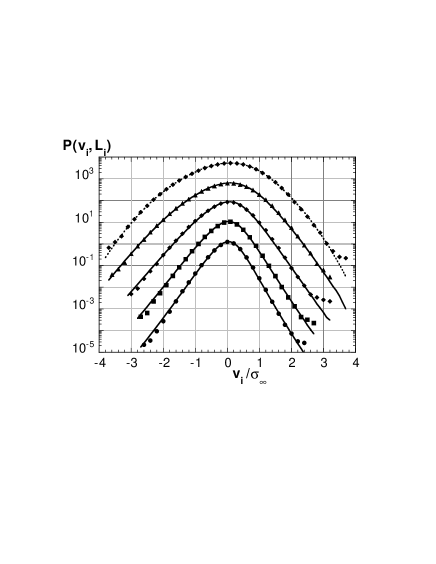
Figure 1: Probability density functions $P(v,L)$ determined from the experimental data (bold symbols) and calculated pdfs (lines) by the numerical iteration with the experimentally determined Fokker-Planck equation (5) and (3). The length scales $\lambda=ln(L_{0}/L)$ were: 0, 0.52, 1.04, 1.56 and 2.24 going from up to down. For the numerical iteration as initial condition an empirical fitting function for the large scale pdf was used which is shown by a broken line. For clarity of presentation the pdfs were shifted in y-direction.

3 Measurement of Kramers-Moyal coefficients

Next, we show how to determine from experimental data appropriate statistical equations to characterize the turbulent cascade. The basic quantity for this procedure is to evaluate the cascade by the statistical dependence of velocity increments of different length scales at the same location $x$ [17]. Either two-increment probabilities $p(v_{2},L_{2};v_{1},L_{1})$ or corresponding conditional probabilities $p(v_{2},L_{2}|v_{1},L_{1})$ are evaluated from the whole data set. (Here we use the convention that $L_{i+1}<L_{i}$.) Investigating the corresponding three-increment statistics we could provide evidence that the evolution of these statistics with different $L_{i}$ fulfill the Chapman-Kolmogorov equation [18, 10, 11]. Furthermore evidences of the validity of the Markov process are shown as long as the step size between different $L_{i}$ is larger than an Markov length $L_{mar}$, which is in the order of some $\eta$ [12]. Thus we know [18] that the evolution of the increments $v_{i}$ is given by a master equation without the involvement of memory functions and that the evolution of the pdfs $P(v_{i},L_{i})$ are described by a Kramers-Moyal expansion:

$$-\frac{d}{dL_{i}}P(v_{i},L_{i})=\sum_{k=1}^{\infty}[-\frac{\partial}{\partial v_{i}}]^{k}D^{(k)}(v_{i},L_{i})\;P(v_{i},L_{i}).$$ (2)

Where the Kramers-Moyal coefficients $D^{(k)}(v_{i},L_{i})$ are defined by the following conditional moments:

$$M^{(k)}(v_{1},L_{1},\delta) = \frac{1}{n!}\frac{1}{\delta}\int\!\!dv_{2}\>(v_{2}-v_{1})^{k}\>p(v_{2},L_{2}|v_{1},L_{1})$$

$$D^{(k)}(v_{1},L_{1}) = \lim_{\delta\rightarrow 0}M^{(k)}(v_{1},L_{1},\delta),$$ (3)

where $\delta=L_{1}-L_{2}$. Knowing the Kramers-Moyal coefficients, and thus the evolution of $P(v_{i},L_{i})$, also the differential equations for the structure functions are obtained easily [10]

$$-\frac{d}{dL}<(v(L))^{q}>=\sum_{n=1}^{q-1}\frac{q!}{(q-n)!}<D^{(n)}v^{q-n}>.$$ (4)

If the Kramers-Moyal coefficients have the form $D^{(q)}=d_{q}v^{q}/L$ (where $d_{q}$ are constants) scaling behavior of (1) is guaranteed with $\zeta_{q}=-\sum_{n=1}^{q-1}\frac{q!}{(q-n)!}d_{n}$. For a discussion of this finding in terms of multifractality and multiaffinity see [19]. The $1/L$ dependence of $D^{(q)}$ indicates that the natural space variable is $lnL$. Thus we take in the following as the space variable $\lambda_{i}=ln(L_{0}/L_{i})$. Furthermore we normalize the velocity increments to the saturation value of $\sigma_{\infty}=\sqrt{<v^{2}_{\infty}>}$ for length scales larger than the integral length.

An important simplification is achieved if the fourth Kramers-Moyal coefficient is zero, than the infinite sum of the Kramers-Moyal expansion (2) reduces to the Fokker-Planck equation of only two terms [18]:

$$\frac{d}{d\lambda}P(v,\lambda)=\left[-\frac{\partial}{\partial v}\tilde{D}^{(1)}(v,\lambda)+\frac{\partial^{2}}{\partial v^{2}}\tilde{D}^{(2)}(v,\lambda)\right]\!P(v,\lambda).$$ (5)

Now only the drift term $\tilde{D}^{(1)}$ and the diffusion term $\tilde{D}^{(2)}$ are determining the statistics completely. Form the corresponding Langevin equation, characterizing the evolution of a spatially fixed increment, we know that $\tilde{D}^{(1)}$ describes the deterministic evolution whereas $\tilde{D}^{(2)}$ describes the noise acting on the cascade. If $\tilde{D}^{(2)}$ shows a v-dependency one speaks of multiplicative noise.

In Fig. 2 we show the evaluated conditional moments $\tilde{M}^{(1)}$ and $\tilde{M}^{(2)}$ as they evolve for $\delta\lambda\rightarrow 0$. For the higher Kramers-Moyal coefficients we found that $\tilde{M}^{(4)}<10^{-2}\tilde{M}^{(2)}$. Thus we take the Fokker-Planck equation as the adequate description.

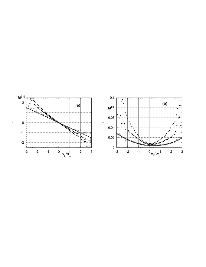
Figure 2: The conditional moments $\tilde{M}^{(1)}(v,\lambda,\delta\lambda)$, (a), and $\tilde{M}^{(2)}(v,\lambda,\delta\lambda)$, (b), for $\lambda=1.48$ and $\Delta\lambda$= 0.04 ($\circ$), 0.06 and 0.20. The fits to the experimental data by polynomial functions (see text) are shown by solid lines. These fits were done only with respect to the interval $-2<v<2)$.

To estimate the $\tilde{D}^{(1)}$ and $\tilde{D}^{(2)}$ coefficient properly we have performed the following three procedures based on the assumption that we can approximate the Kramers-Moyal coefficient by the following polynomials: $\tilde{D}^{(1)}=\gamma(\lambda)$ and $\tilde{D}^{(2)}=\alpha(\lambda)+\delta(\lambda)*v_{i}+\beta(\lambda)*v_{i}^{2}$. At first, we used the same polynomial forms for the $\tilde{M}$-coefficients and estimated the coefficients of the polynomials for $\delta\lambda\rightarrow 0$. Here problems arise due to the finite value of the Markov-length and due to the finite resolution of our detector. Secondly, inserting the polynomials of $\tilde{D}^{(1)}$ and $\tilde{D}^{(2)}$ into (4) we can determine directly the coefficients $\alpha$ to $\delta$ from the measured structure functions (the highest order of the structure function we used was 6). Problems arise due to the noise of the derivative of the structure functions, thus only the magnitude of the coefficient could be estimated. Thirdly, we have evaluated analogously the corresponding structure functions of $P_{even}(v,L)=1/2(P(v,L)+P(-v,L))$ and $P_{odd}(v,L)=1/2(P(v,L)-P(-v,L))$. [20]

From all these estimations we got a good guess of the values of $\alpha(\lambda)$ to $\delta(\lambda)$. The best results we obtained for $\gamma$. The worst result was obtained for $\beta$, for which we finally used the value $\mu/18$ expected from the Kolmogorov picture of intermittency [21, 10]. As the final values we got:

$$\gamma(\lambda) = 0.36exp\left\{(\frac{\lambda-0.68}{2.1})^{3}\right\}$$

$$\alpha(\lambda) = 0.02exp\left\{-\frac{\lambda}{1.3}\right\}$$

$$\delta(\lambda) = 0.013exp(-1.2\lambda)$$

$$\beta = 0.017\qquad.$$ (6)

Next, let us briefly comment this result. For $\gamma$ we find that it has a constant value of 1/3 in the inertial range ($0<\lambda<2$). The functional dependence of $\gamma$ is given to extend the $\lambda$ dependence into the dissipation range. The values $\delta$ and $\alpha$ are violating scaling behavior. Both, $\alpha$ and $\delta$, are decaying exponentially with $\lambda$. For scales larger than the integral length these two coefficients are large and are responsible for the building up of the skewness, because these terms allow the change of the sign of the velocity increments within the stochastic process.

As further test of the validity of our approach we have calculated the evolution of the pdfs by a numerical iteration with the Fokker-Planck equation. As an initial condition the pdf $P(v_{0},L_{0})$ at the integral scale was approximated by an empirical function and then inserted into the numerical iteration. We found that the evolution of the pdfs depends sensitively on the chosen coefficients. (Finally, we changed the numbers in (LABEL:coeaff) in the range of some percent to obtain a best result.) The result of the numerical iteration of the Fokker-Planck equation with the above mentioned coefficients are shown in Fig. 1 by solid lines.

4 Universality

Let us now discuss how the turbulent cascade will be affected, if the statistics on large scales is changed as it may be the case for different driving forces. As an extreme case we have chosen a box like form for a large scale pdf (the standard deviation and the skewness was adapted to the one of our experimental pdf for $L_{0}$ (see Fig. 3)). Next, using the above mentioned coefficients (3), we have iterated simultaneously the experimental approximation of $P(v_{0},L_{0})$, see Fig. 1, and the box like pdf. As shown in Fig.3 we see that under the iteration the synthetic pdf becomes more and more similar to the experimental ones. This convergence has been quantified by the $\chi^{2}$ measure ($\chi^{2}\propto\sum(P_{1}-P_{2})^{2}/P_{1}$ ). We find that $\chi^{2}$ decays about exponentially with $\lambda$. Thus, we see that for a sufficient large cascade any large scale pdf will converge against universal small scale pdfs.

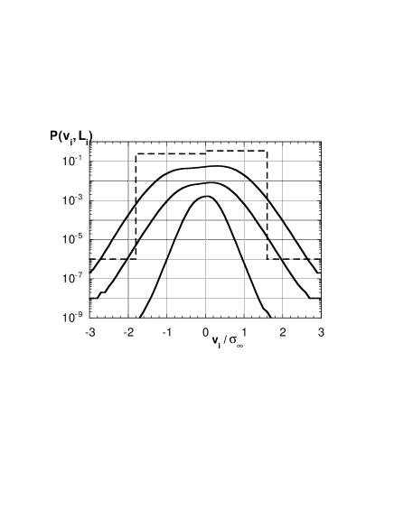
Figure 3: Evolution of a synthetic box-shaped pdf (broken line) under the numerical integration with the Fokker-Planck equation using the coefficients of (3). From top to bottom $\lambda=$ 0, 1.4, 2.2 and 3.0. Presentation as in Fig.1.

5 Conclusion

We have presented further evidence that the statistics of fully developed turbulence is based on a Markov process in the space variable $L$. It has been shown how the drift coefficient and the diffusion coefficient of a describing Fokker-Planck equation can be determined from experimental data. With these coefficients it is possible to calculate accurately the pdfs of a cascade. As a further result we have shown that situations where the large scale statistics differ, for example due to different driving forces, will show the same small scale statistics, as long as the same Fokker-Planck equations apply. Therefore, universality of small scale turbulence can best be characterized by comparing the drift and diffusion coefficients.

The next challenging questions are, how do these result depend on the Reynolds number and what happen in anisotropic turbulence. For the ladder point recently evidence has been found that for sufficiently small scales again the results of local isotropic turbulence hold [22]. We believe that these findings do not only play an important role for the complete statistical characterization of turbulence but also should have quite practical importance for numerical simulations of flow situations with high Reynolds numbers.

6 Acknowledgments

We want to acknowledge discussions with A. Naert, P. Talkner, K. Zeile, H. Brand. J.P. acknowledges the financial support of the Deutsche Forschungsgemeinschaft.

References

- [1] A.S.Monin, A.M. Yaglom, Statistical Fluid Mechanics, (MIT Press, Cambridge 1975).
- [2] U. Frisch, Turbulence (Cambridge 1995).
- [3] R. Benzi, S. Ciliberto, C. Baudet,G.R. Chavarria, Physica D 80, 385 (1995).
- [4] A. Arneodo, et. al. Europhys. Lett. 34, 411 (1996).
- [5] K.R. Sreenivasan, R.A. Antonia, Annu. Rev. Fluid Mech. 29, 435 (1997).
- [6] R. Benzi, L. Biferale, G. Paladin, A. Vulpiani, M. Vergassola, Phys. Rev. 67, 2299 (1991); P. Kailasnath, K.R. Sreenivasan, G. Stolovitzky, Phys. Rev. 68, 2767 (1992).
- [7] B. Castaing, Y. Gagne, E. Hopfinger, Physica D 46, 177 (1990).
- [8] H. Tennekes, J.C. Wyngaard, J. Fluid Mech. 55, 93 (1972);F. Anselmat, Y. Gagne, E.J. Hopfinger, R.A. Antonia, J. Fluid. Mech 149,63 (1984); J. Peinke, B. Castaing, B. Chabaud, F. Chilla, B. Hebral, A. Naert, in Fractals in the Natural and Applied Sciences, edt.: M.M. Novak (North Holland, Amsterdam 1994) p.295.
- [9] R.A. Antonia, B.R. Satyaprakash, A.K.M.F. Hussain, J. Fluid Mech. 119, 55 (1982); B. Castaing, Y. Gagne, E.J. Hopfinger, A new View of Developed Turbulence, in New Approaches and Concepts in Turbulence, Edts. Th. Dracos and A. Tsinober (Birkhäuser, Basel 1993) see also Discussion p. 47 - 60 therein; B. Castaing, Y. Gagne, M. Marchand, Physica D 68, 387 (1993). B. Chabaud, A. Naert, J. Peinke, F. Chilla, B. Castaing, B. Hebral, Phys. Rev. Lett. 73 (1994) 3227;
- [10] R. Friedrich, J. Peinke, Phys. Rev. Lett. 78,863 (1997); A. Naert,R. Friedrich, J. Peinke, Phys. Rev. E 56, 6719 (1997).
- [11] R. Friedrich, J. Peinke, Physica D 102, 147 (1997).
- [12] R. Friedrich, J. Zeller, J. Peinke, Europhys. Lett. 41, 143 (1998).
- [13] It has recently been shown that in an analogous way it is possible to analyse dynamical systems, and to extract the Langevin equation directly from a given data set; S. Siegert, R. Friedrich, J. Peinke (preprint).
- [14] N. Rajartnan, Turbulent Jets (Elsevier, Amsterdam 1976); Ch. Renner, Diplomarbeit (Bayreuth 1997).
- [15] B. Bümel and H.E. Fiedler (Berlin) priv. communication.
- [16] D. Aronson, L. Lofdahl, Phys. Fluids A5, 1433 (1993).
- [17] J. Peinke, R. Friedrich, F. Chilla, B. Chabaud, and A. Naert, Z. Phys. B 101, 157 (1996).
- [18] H. Risken, The Fokker-Planck Equation, (Springer-Verlag Berlin, 1984); P. Hänggi and H. Thomas, Physics Reports 88, 207 (1982).
- [19] J. Peinke, R. Friedrich, A. Naert, Z. Naturforsch. 52a, 588 (1997).
- [20] The Fokker-Planck equations for and have the same form as (5), only if the coefficient , this may clear up the question of the sense of evaluating moments of the absolute values of , see for example footnote on page 446 in [5].
- [21] A.M. Oboukhov, J. Fluid Mech. 13, 77 (1962); A.N. Kolmogorov J. Fluid Mech. 13, 82 (1962).
- [22] F. Chilla et.al. to be published