Cascades and statistical equilibrium in shell models of turbulence

Abstract

We study the GOY shell model simulating the cascade processes of turbulent flow. The model has two inviscid invariants governing the dynamical behavior. Depending on the choice of interaction coefficients, or coupling parameters, the two invariants are either both positive definite, analogous to energy and enstrophy of 2D flow, or only one is positive definite and the other not, analogous to energy and helicity of 3D flow. In the 2D like model the dynamics depend on the spectral ratio of enstrophy to energy. That ratio depends on wave-number as $k^{\alpha}$. The enstrophy transfer through the inertial sub-range can be described as a forward cascade for $\alpha<2$ and a diffusion in a statistical equilibrium for $\alpha>2$. The $\alpha=2$ case, corresponding to 2D turbulence, is a borderline between the two descriptions. The difference can be understood in terms of the ratio of typical timescales in the inertial sub-range and in the viscous sub-range. The multi fractality of the enstrophy dissipation also depends on the parameter $\alpha$, and seems to be related to the ratio of typical timescales of the different shell velocities.

I Introduction

The standard Kolmogorov $k^{-5/3}$ scaling law for energy cascading in 3D turbulence and the corresponding $k^{-3}$ scaling law for enstrophy cascade in 2D turbulence is still debated. Direct numerical calculations of the full Navier-Stokes equation is by and large still impossible for high Reynolds number $(>100-200)$ flows. However, the cascading mechanisms and its multi fractal nature can be analyzed in reduced wave-number models for very high Reynold numbers with high accuracy. In this paper we investigate the GOY shell model [1, 2] where the spectral velocity or vorticity is represented by one complex variable for each shell evenly spaced in $log(k)$ in spectral space. For this type of model the Kolmogorov scaling arguments can be applied as for real flow regardless of how realistically they mimic the dynamics of the Navier-Stokes equation. The scaling behavior of the fields depends on the inviscid invariants of the model. In the simple model we are able to control which symmetries and conserved integrals of the dynamics that are present in the inviscid and force-free limit. In the models we interpret as simulating 3D turbulence there are 2 inviscid invariants, similar to energy and helicity [3], of which the first is positive definite and the second is not. For the models we interpret as 2D turbulence the 2 inviscid invariants, similar to energy and enstrophy, are both positive definite. We will mainly be concerned with an investigation of the 2D like models. The specific parameter choice previously assigned to simulating 2D turbulence are such that the GOY model does not show enstrophy cascading but rather a statistical equilibrium where the enstrophy is transported through the inertial sub-range by diffusion [4]. We show that this is a borderline case for which, on one side, the model behaves as a cascade model and, on the other side, it behaves as a statistical equilibrium model, where the enstrophy spectrum is characterized by a simple equipartitioning among the degrees of freedom of the model. The difference in behavior is connected with the different typical timescales of the shell velocities as function of shell number. This probabily also influences the (non-universal) multi fractal behavior of the shell velocities. If timescales in the viscous sub-range are not smaller than in the beginning of the inertial sub-range,the low wave-number end, the model does not have a multi fractal spectrum.

II The GOY model

The GOY model is a simplified analogy to the spectral Navier-Stokes equation for turbulence. The spectral domain is represented as shells, each of which is defined by a wavenumber $k_{n}=k_{0}\lambda^{n}$, where $\lambda$ is a scaling parameter defining the shell spacing; in our calculations we use the standard value $\lambda=2$. The reduced phase space enables us to cover a large range of wavenumbers, corresponding to large Reynolds numbers. We have $2N$ degrees of freedom, where $N$ is the number of shells, namely the generalized complex shell velocities or vorticities, $u_{n}$ for $n=1,N$. The dynamical equation for the shell velocities is,

$$\dot{u}_{n}=ik_{n}(au^{*}_{n+2}u^{*}_{n+1}+\frac{b}{\lambda}u^{*}_{n+1}u^{*}_{n-1}+\frac{c}{\lambda^{2}}u^{*}_{n-1}u^{*}_{n-2})-\nu k_{n}^{p_{1}}u_{n}-\nu^{\prime}k_{n}^{-p_{2}}u_{n}+f_{n},$$ (1)

where the first term represents the non-linear wave interaction or advection, the second term is the dissipation, the third term is a drag term, specific to the 2D case, and the fourth term is the forcing. Throughout this paper we use $p_{1}=p_{2}=2$. We will for convenience set $a=k_{0}=1$, which can be done in (1) by a rescaling of time and the units in $k$ space. A real form of the GOY model, as originally proposed by Gledzer [1], can be obtained trivially by having purely imaginary velocities and forcing. The GOY model in its original real form contains no information about phases between waves, thus there cannot be assigned a flow field in real space to the spectral field. The complex form of the GOY model and extensions in which there are more shell variables in each shell introduce some degrees of freedom, which could be thought of as representing the phases among waves. However, it seems as if these models do not behave differently from the real form of the model in regard to the conclusions in the following [5, 4]. The key issue for the behavior of the model is the symmetries and conservation laws obeyed by the model.

A Conservation laws

The GOY model has two conserved integrals, in the case of no forcing and no dissipation $(\nu=f=0)$. We denote the two conserved integrals by

$$E^{1,2}=\sum_{n=1}^{N}E^{1,2}_{n}=\frac{1}{2}\sum_{n=1}^{N}k_{n}^{\alpha_{1,2}}|u_{n}|^{2}=\frac{1}{2}\sum_{n=1}^{N}\lambda^{n\alpha_{1,2}}|u_{n}|^{2}$$ (2)

By setting $\dot{E}^{1,2}=0$ and using $\dot{u}_{n}$ from (1) we get

$\displaystyle\left\{\begin{array}[]{ll}1+bz_{1}+cz_{1}^{2}=0\\ 1+bz_{2}+cz_{2}^{2}=0,\end{array}\right.$

(3)

where the roots $z_{1,2}=\lambda^{\alpha_{1,2}}$ are the generators of the conserved integrals. In the case of negative values of $z$ we can use the complex formulation, $\alpha=(log|z|+i\pi)/log\lambda$. The parameters $(b,c)$ are determined from (3) as

$\displaystyle\left\{\begin{array}[]{ll}b=-(z_{1}+z_{2})/z_{1}z_{2}\\ c=1/z_{1}z_{2}.\end{array}\right.$

(4)

In the $(b,c)$ parameter plane the curve $c=b^{2}/4$ represents models with only one conserved integral, see figure 1. Above the parabula the generators are complex conjugates, and below they are real and different. Any conserved integral represented by a real nonzero generator $z$ defines a line in the $(b,c)$ parameter plane, which is tangent to the parabula in the point $(b,c)=(-2/z,1/z^{2})$. The rest of our analysis we will focus on the line defined by $z_{1}=1$. The conserved integral,

$$E^{1}=\frac{1}{2}\sum_{n=1}^{N}|u_{n}|^{2},$$ (5)

is the usual definition of the energy for the GOY model [3]. The parameters are then determined by $1+b+c=0$, which with the definitions $b=-\epsilon$ and $c=-(1-\epsilon)$ agree with the notation of ref. [6]. The generator of the other conserved integral is from (4) given as,

$$z_{2}=\frac{1}{\epsilon-1}.$$ (6)

For $\epsilon<1$ the second conserved integral is not positive definite and is of the form,

$$E^{2}=H=\frac{1}{2}\sum_{n=1}^{N}(-1)^{n}|z_{2}|^{n}|u_{n}|^{2},$$ (7)

which can be interpreted as a generalized helicity. For $\epsilon=1/2$, $z_{2}=-2=-\lambda$ the model is the usual 3D shell model and H is the helicity as defined in ref. [3]. By choosing $\lambda$ such that $\lambda=1/(1-\epsilon)$ we get $E^{2}=\sum(-1)^{n}\lambda^{n}|u_{n}|^{2}$. This form was argued in ref. [3] to be the proper form for the helicity. In this paper we will alternatively use the definition (7) for the helicity.

For $\epsilon>1$ the second conserved integral is positive definite and of the form,

$$E^{2}=Z=\frac{1}{2}\sum_{n=1}^{N}z_{2}^{n}|u_{n}|^{2},$$ (8)

which can be interpreted as a generalized enstrophy. For $\epsilon=5/4$, $z_{2}=4=\lambda^{2}$ the model is the usual 2D shell model and Z is the enstrophy as defined in ref. [4]. The sign of $c$, which is the interaction coefficient for the smaller wavenumbers, changes when going from the 3D - to the 2D case. This could be related to the different role of backward cascading in the two cases. To see this, consider the non-linear transfer of $E^{i}$ through the triade interaction between shells, $n-1,n,n+1$. This is simply given by,

$$\dot{E}^{i}_{n-1} = k^{\alpha_{i}}_{n-1}\Delta_{n}$$ (9)

$$\dot{E}^{i}_{n} = bz_{i}k^{\alpha_{i}}_{n-1}\Delta_{n}$$ (10)

$$\dot{E}^{i}_{n+1} = cz_{i}^{2}k^{\alpha_{i}}_{n-1}\Delta_{n},$$ (11)

with

$$\Delta_{n}=k_{n-1}Im(u_{n-1}u_{n}u_{n+1}).$$ (12)

The detailed conservation of $E^{i}$ in the triade interaction is reflected in the identity, $1+bz_{i}+cz_{i}^{2}=0$. Using (4) and (6) we have for the exchange of energy, $E^{1}$, with $\alpha_{1}=0$;

$$\dot{E}^{1}_{n-1} = \Delta_{n}$$ (13)

$$\dot{E}^{1}_{n} = -\epsilon\Delta_{n}$$ (14)

$$\dot{E}^{1}_{n+1} = (\epsilon-1)\Delta_{n}$$ (15)

and for helicity/enstrophy, $E^{2}$, with $\alpha_{2}=\alpha$;

$$\dot{E}^{2}_{n-1} = k^{\alpha}_{n-1}\Delta_{n}$$ (16)

$$\dot{E}^{2}_{n} = -(\epsilon/(\epsilon-1))k^{\alpha}_{n-1}\Delta_{n}$$ (17)

$$\dot{E}^{2}_{n+1} = (1/(\epsilon-1))k^{\alpha}_{n-1}\Delta_{n}.$$ (18)

We have $\epsilon<1$ for 3D like models and $\epsilon>1$ for 2D like models, the two situations are depicted in figure 2, where the thickness of the arrows symbolize the relative sizes of the exchanges in the cases of $\epsilon=1/2$ and $\epsilon=5/4$.

B Scaling and inertial range.

The inertial sub-range is defined as the range of shells where the forcing and the dissipation are negligible in comparison with the non-linear interactions among shells. Since we apply the forcing at the small shell numbers and the dissipation at the large shell numbers, the inertial range (of forward cascade) is characterized by the constant cascade of one of the conserved quantities. The classical Kolmogorov scaling analysis can then be applied to the inertial range. There is, however, in the shell model, long range influences of the dissipation and forcing into the inertial subrange. This is an artifact of the modulus 3 symmetry, see equation (28), and the truncation of the shell model which is not expected to represent any reality. These features are treated in great detail in ref. [9]. Denoting $\eta_{1,2}$ as the average dissipation of $E^{1,2}$, this is then also the amount of $E^{1,2}$ cascaded through the inertial range. The spectrum of $E^{1,2}$ does then, by the Kolmogorov hypothesis, only depend on $k$ and $\eta_{1,2}$. From dimensional analysis we have, $[ku]=s^{-1}$, $[\eta_{1,2}]=[E^{1,2}]s^{-1}$, $[E^{1,2}]=[k^{\alpha_{1,2}}u^{2}]=[k]^{\alpha-2}s^{-2}$, and we get,

$$E^{1,2}\sim\eta_{1,2}^{2/3}k^{(\alpha_{1,2}-2)/3}.$$ (19)

For the generalized velocity, $u$, we then get the ”Kolmogorov- scaling”,

$$|u|\sim\eta_{1,2}^{1/3}k^{-(Re(\alpha_{1,2})+1)/3}.$$ (20)

The non-linear cascade, or flux, of the conserved quantities defined by $z_{1,2}$ through shell number $n$ can be expressed directly as,

$$\Pi_{n}^{1,2}=\sum_{m=1}^{n}\dot{E}^{1,2}(m) = \frac{1}{2}\sum_{m=1}^{n}z_{1,2}^{m}(u^{*}_{m}\dot{u}_{m}+c.c.)$$ (21)

$$= z_{1,2}^{n}(-\Delta_{n}/z_{2,1}+\Delta_{n+1}).$$ (22)

In the inertial range the cascade is constant, $\Pi_{n}^{1,2}=\Pi_{n+1}^{1,2}$, so from (22) we get following ref. [6]

$$z_{1}z_{2}\Delta_{n+2}-(z_{1}+z_{2})\Delta_{n+1}+\Delta_{n}=0\Rightarrow$$ (23)

$$q_{n}+z_{1}z_{2}/q_{n+1}=z_{1}+z_{2}$$ (24)

where we have defined

$$q_{n}=\Delta_{n}/\Delta_{n+1}.$$ (25)

The inertial range scaling requires $q_{n}=q_{n+1}=q$ to be independent of $n$. Solving (24) for $q$ and using (25) gives,

$\displaystyle q=\left\{\begin{array}[]{ll}z_{1}\Rightarrow u_{n}\sim k_{n}^{-(\alpha_{1}+1)/3}&\mbox{Kolmogorov for $E^{1}$}\\ z_{2}\Rightarrow u_{n}\sim k_{n}^{-(\alpha_{2}+1)/3}&\mbox{Kolmogorov for $E^{2}$}.\end{array}\right.$

Inserting this into (22) gives for the cascade of $E^{1}$ in the two solutions,

$\displaystyle\Pi^{1}\sim\left\{\begin{array}[]{ll}1-z_{2}/z_{1}&\mbox{Kolmogorov for $E^{1}$}\\ 0&\mbox{fluxless for $E^{1}$,}\end{array}\right.$

(26)

and correspondingly for $E^{2}$,

$\displaystyle\Pi^{2}\sim\left\{\begin{array}[]{ll}0&\mbox{fluxless for $E^{2}$}.\\ 1-z_{1}/z_{2}&\mbox{Kolmogorov for $E^{2}$}.\end{array}\right.$

These are the two scaling fixed points for the model. The Kolmogorov fixed point for the first conserved integral corresponds to the fluxless fixed point for the other conserved integral and visa versa. This is of course reflected in the fact that (24) is symmetric in the indices 1 and 2. That these points in phase space are fixed points, in the case of no forcing and dissipation, is trivial, since $\Pi_{n}=\Pi_{n+1}\Rightarrow\dot{E}_{n+1}=0\Rightarrow\dot{u}_{n+1}=0$. It should be noted that the Kolmogorov fixed point,

$$u\sim k^{-(\alpha+1)/3},$$ (27)

obtained from this analysis is in agreement with the dimensional analysis (19).

The scaling fixed points can be obtained directly from the dynamical equation as well. For $u_{n}\sim k_{n}^{-\gamma}g(n)=\lambda^{-n\gamma}g(n)$, where $g(n+3)=g(n)$ is any period 3 function, we get by inserting into (1) with $a=1$,

$$g(n-1)g(n)g(n+1)\lambda^{n(1-\gamma)+3\gamma}(1+b\lambda^{3\gamma-1}+c(\lambda^{3\gamma-1})^{2})=0$$ (28)

and the generators reemerge, $z_{1,2}=\lambda^{\alpha_{1,2}}=\lambda^{3\gamma_{1,2}-1}$, giving the Kolmogorov fixed points for the two conserved integrals, $\gamma_{1,2}=(\alpha_{1,2}+1)/3$.

The period 3 symmetry seems to have little implications for the numerical integrations of the model, except perhaps in accurately determining the structure function.

The stability of the fixed point for energy cascade in the 3D case, $\epsilon=1/2$, is characterized by few unstable directions, where the corresponding eigenmodes mainly projects onto the high shell numbers, and a large number of marginally stable directions which mainly projects onto the inertial range. This also holds in the case with forcing and dissipation [8]. In the case where dissipation and forcing are applied for some values of $\epsilon$ the Kolmogorov fixed point can become stable. Biferale et al. [6] show that there is a transition in the GOY model, for $\nu=10^{-6}$ and $f=5\times 10^{-3}\times(1+i)$, as a function of $\epsilon$ from stable fixed point $(\epsilon<0.38..)$, through Hopf bifurcations and via a Ruelle-Takens scenario to chaotic dynamics $(\epsilon>0.39..)$.

III Forward and backward cascades

Until this point we have not specified which of the two conserved quantities will cascade. Assume, in the chaotic regime where the Kolmogorov fixed points are unstable, that there is, on average, an input of the same size of the two quantities, $E^{1}$ and $E^{2}$, at the forcing scale, this can of course always be done by a simple rescaling of one of the quantities. If $N_{d}$ is a shell number at the beginning of the viscous subrange, we have that $u_{N_{d}}/k_{N_{d}}\approx\nu$,and the dissipation, $D^{i}$, of the conserved quantity, $E^{i}$, can be estimated as

$$D^{i}\sim\nu k_{N_{d}}^{\alpha_{i}+2)}|u_{N_{d}}|^{2}.$$ (29)

The ratio of dissipation of $E^{1}$ and $E^{2}$ scales with $k_{N_{d}}$ as $D^{1}/D^{2}\sim k_{N_{d}}^{\alpha_{1}-\alpha_{2}}$, so that, in the limit $Re\rightarrow\infty$ when $\alpha_{1}<\alpha_{2}$, there will be no dissipation in the viscous sub-range of $E^{1}$ where $E^{2}$ is dissipated. Therefore, a forward cascade of $E^{1}$ is prohibited and we should expect a forward cascade of $E^{2}$. For the backward cascade the situation is reversed, so we should expect a backward cascade of $E^{1}$.

The situation is completely different in the 2D like and the 3D like cases. In the 3D like models $E^{2}$ is not positive definite, $E^{2}$ (helicity) is generated also in the viscous sub-range and for the usual GOY model we do not see a forward cascade of helicity, see, however, ref. [7]. This is in agreement with the observed $k^{-5/3}$ energy spectrum observed in real 3D turbulence corresponding to the forward cascade of energy. In the 2D case we observe the direct cascade of enstrophy, while the inverse cascade of energy is still debated. In the rest of this paper we will concentrate on 2D like models where we will implicitly think of $E^{1}=E$, with $\alpha_{1}=0$, as the energy and $E^{2}=Z$, with $\alpha_{2}=\alpha>0$, as the enstrophy. With regard to the inverse cascade of energy one must bare in mind that in 2D turbulence the dynamics involved is probably related to the generation of large scale coherent structures, vortices, and vortex interactions. Vortices are localized spatially, thus delocalized in spectral space. This is in agreement with the estimate that 2D is marginally delocalized in spectral space [11]. In the GOY model there is no spatial structure and the interactions are local in spectral space. The model is therefore probably not capable of showing a realistic inverse energy cascade. We will thus only consider the forward cascade in this paper. Figure 3 shows the scaling in the inertial sub-range of the model with $\epsilon=5/4$ corresponding to $\alpha=2$. The cascades of the enstrophy and energy are shown in figure 4. It is seen that enstrophy is forward cascaded while energy is not.

IV Statistical description of the model

In a statistical equilibrium of an ergodic dynamical system we will have a probability distribution among the (finite) degrees of freedom, assuming an ultraviolet cutoff, of the form, $P_{i}\sim\exp(-BE_{i}^{1}-AE_{i}^{2})$, where $E^{1}$ and $E^{2}$ are the conserved quantitied, energy and enstrophy. Thus, the temporal mean of any quantity, which is a function of the shell velocities is given as

$$\overline{g}=\int\prod_{i}du_{i}g(u_{1},...,u_{N})\exp(-BE_{i}^{1}-AE_{i}^{2})/\int\prod_{i}du_{i}\exp(-BE_{i}^{1}-AE_{i}^{2}).$$ (30)

$A$ and $B$ are Lagrange multipliers, reflecting the conservation of energy and enstrophy when maximizing the entropy of the system, corresponding to inverse temperatures, denoted as inverse ”energy-” and ”enstrophy-temperatures” [10]. The shell velocities themselves will in this description be independent and gaussian distributed variables with standard deviation $\sigma(u_{i})=1/(2(Bk_{i}^{\alpha_{1}}+Ak_{i}^{\alpha_{2}}))$. The average values of the energy and enstrophy becomes,

$$\overline{E_{i}^{1}}=k_{i}^{\alpha_{1}}\overline{|u_{i}|^{2}}=(B+Ak_{i}^{\alpha_{2}-\alpha_{1}})^{-1}$$ (31)

$$\overline{E_{i}^{2}}=k_{i}^{\alpha_{2}}\overline{|u_{i}|^{2}}=(Bk_{i}^{\alpha_{1}-\alpha_{2}}+A)^{-1}.$$ (32)

For $k\rightarrow 0$ we will have equipartitioning of energy, $k_{i}^{\alpha_{1}}\overline{|u_{i}|^{2}}=B^{-1}$ and the scaling $|u_{i}|\sim k_{i}^{-\alpha_{1}/2}$ and for the other branch, $k\rightarrow\infty$, we will have equipartitioning of enstrophy $k_{i}^{\alpha_{2}}\overline{|u_{i}|^{2}}=A^{-1}$ and the scaling $|u_{i}|\sim k_{i}^{-\alpha_{2}/2}$. In the case of no forcing and no viscosity the equilibrium will depend on the ratio $A/B$ between the initial temperatures $A^{-1},B^{-1}$. To illustrate this we ran the model without forcing and viscosity but with 2 different initial spectral slopes of the velocity fields, the larger the slope the higher the ratio of the energy temperature to the enstrophy temperature. Figure 5 shows the equilibrium spectra for $\epsilon=5/4,\nu=f=0$, in the cases of initial slopes -1, -0.8. The full lines are the equilibrium distribution given by (32) for $A/B=10^{2}$ and $A/B=10^{-2}$ respectively.

V Distinguishing cascade from statistical equilibrium

For the forward enstrophy cascade the spectral slope is $-(\alpha+1)/3$ and the enstrophy equipartitioning branch has spectral slope $-\alpha/2$. Thus for the 2D case where $\alpha=2$ we cannot distinguish between statistical (quasi-) equilibrium and cascading. This was pointed out by Aurell et al. [4] and it was argued that the model can be described as being in statistical quasi-equilibrium with the enstrophy transfer described as a simple diffusion rather than an enstrophy cascade. This coinciding scaling is a caviate of the GOY model not present in the real 2D flow where the statistical equilibrium energy spectrum scales as $k^{-1}$ and the cascade energy spectrum scales as $k^{-3}$. For other values of $\alpha$ the scaling of the two cases are different, see figure 6. This figure represents the main message of this paper. First axis is the parameter $\epsilon$, along the line shown in fig. 1, defining the spectral ratio between the two inviscid invariants. Second axis is the scaling exponent $\gamma$. The horizontal dashed line $\gamma=1/3$ is the Kolmogorov scaling exponent for energy cascade. The full curve is the scaling exponent for the enstrophy cascade, and the dotted curve corresponds to the enstrophy equipartitioning.

All the 3D like models (asterisks in figure 6) are near energy cascade scaling (dashed line). Statistical equilibrium corresponds to the line $\gamma=0$. The bold line piece, $0<\epsilon<0.39...$, represents parameter values where the Kolmogorov fixed point is stable [6]. The scaling for $\epsilon>0.39...$ is slightly steeper than the Kolmogorov scaling, which is attributed to intermittency corrections originating from the viscous dissipation [12]. It seems as if there is a slight trend showing increasing spectral slopes for increasing $\epsilon$.

For the 2D like models the scaling slope is also everywhere on or slightly above both the cascade - and the equilibrium slopes (diamonds in the figure). The classical argument for a cascade is that given an initial state with enstrophy concentrated at the low wave-number end of the spectrum, the enstrophy will flow into the high wave-numbers in order to establish statistical equilibrium. The ultra-violet catastrophe is then prevented by the dissipation in the viscous sub-range. Therefore, we cannot have a non-equilibrium distribution with more enstrophy in the high wave-number part of the spectrum than prescribed by statistical equilibrium since enstrophy in that case would flow from high - to low wave-numbers. This means that the spectral slope in the inertial sub-range always is above the slope corresponding to equilibrium (dotted line in figure 6). Consequently, the 2D model with $\epsilon=5/4$ separates two regimes, $1<\epsilon<5/4$ where enstrophy equilibrium is achieved and $5/4<\epsilon<2$ where the enstrophy is cascaded through the inertial range.

In figure 7 the spectra and the cascades are shown for different values of $\epsilon$. The model was run with 50 shells and forcing on shell number 15 for $2\times 10^{4}$ time units and averaged. Even then there are large fluctuations in the cascades not reflected in the spectra. The large differences in the absolut values for the cascades, $Pi$, is a reflection of the scaling relation (29).

We interpret the peaks around the forcing scale for $\epsilon=11/10$ as statistical fluctuation and the model shows no cascade. For $\epsilon>5/4$ we see an enstrophy cascade and what seems to be an inverse energy cascade. However, we must stress that we do not see a second scaling regime for small $n$ corresponding the inverse cascade. Note that for $\epsilon=2$ energy and enstrophy are identical and we have only one inviscid invariant. So if a regime of inverse energy cascading existed in parameter space near $\epsilon=2$ the scaling exponents will be almost identical and coincide at $\epsilon=2$.

The two regimes corresponding to equipartitioning and cascade can be understood in terms of timescales for the dynamics of the shell velocities. A rough estimate of the timescales for a given shell $n$, is from (1) given as $T_{n}\sim(k_{n}u_{n})^{-1}\sim k_{n}^{\gamma-1}$. Again $\epsilon=5/4$, corresponding to $\gamma=1$, becomes marginal where the timescale is independent of shell number. For $\epsilon<5/4$ the timescale grows with $n$ and the fast timescales for small $n$ can equilibrate enstrophy among the degrees of freedom of the system before the dissipation, at the ”slow” shells, has time to be active. Therefore these models exhibits statistical equilibrium. For $\epsilon>5/4$ the situation is reversed and the models exhibits enstrophy cascades. Time evolutions of the shell velocities are shown in figure 8, where the left columns show the evolution of a shell in the beginning of the inertial subrange and the right columns show the evolution of a shell at the end of the inertial subrange. This timescale scaling might also explain why no inverse cascade branch has been seen in the GOY model. The timescales at the small wave-number end of the spectrum, with the dissipation or drag range for inverse cascade, is long in comparison with the timescales of the inertial range of inverse cascade. Therefore a statistical equilibrium will have time to form. The analysis suggests that parameter choices $\epsilon>5/4$ might be more realistic than $\epsilon=5/4$ for mimicing enstrophy cascade in real 2D turbulence.

VI Intermittency corrections

The numerical result that the inertial range scaling has a slope slightly higher than the K 41 prediction, is not fully understood. This is attributed to intermittency corrections originating from the dissipation of enstrophy in the viscous subrange.

The evolution of the shell velocities in the viscous sub-range is intermittent for $\epsilon>5/4$, where the PDF’s are non-gaussian, while the PDF’s for $\epsilon=5/4$ are gaussian in both ends of the inertial sub-range, see figure 9. The deviation from the Kolmogorov scaling is expressed through the structure function, $\zeta(q)$ [12]. The structure function is defined through the scaling of the moments of the shell velocities;

$$\overline{|u_{n}|^{q}}\sim k_{n}^{\zeta(q)}=k_{n}^{-q\gamma-\delta\zeta(q)}$$ (33)

where $\delta\zeta(q)$ is the deviation from Kolmogorov scaling. The structure function, $\zeta(q)$, and $\delta\zeta(q)$ for $\epsilon=11/10,5/4,3/2,7/4,2$ are shown in figure 10. For $\epsilon>5/4$ there are intermittency corrections to the scaling in agreement with what the PDF’s show.

We know of no analytic way to predict the intermittency corrections from the dynamical equation. Our numerical calculations suggest that the intermittency corrections are connected with the differences in typical timescales from the beginning of the inertial sub-range, where the model is forced, to the viscous sub-range. The ratio of timescales between the dissipation scale and the forcing scale can be estimated by; $T_{\nu}/T_{f}\approx\lambda^{\Delta N(1+\gamma)}$, where $\Delta N$ is the number of shells beween the two. Figure 11 (a) shows the numerical values of $\delta\zeta(10)$ as a function of $\epsilon$ and figure 11 (b) shows $log_{2}(T_{\nu}/T_{f})$ as a function of $\epsilon$. The vertical line indicates the crossover between statistical equilibrium and cascading. We must stress that caution should be taken upon drawing conclusions from this since the authors have no physical explanation of the appearent relationship.

VII Summary

The GOY shell model has two inviscid invariants, which govern the behavior of the model. In the 2D like case these corresponds to the energy and the enstrophy of 2D turbulent flow. In the model we can change the interaction coefficient, $\epsilon$, and tune the spectral ratio of enstrophy to energy, $Z_{n}/E_{n}=k_{n}^{\alpha}$. For $\alpha>2$ we can describe the dynamics as being in statistical equilibrium with two scaling regimes corresponding to equipartitioning of energy and enstrophy respectively. The reason for the equipartitioning of enstrophy in the inertial range (of forward cascading of enstrophy) is that the typical timescales, corresponding to eddy turnover times, are growing with shell number, thus the timescale of viscous dissipation is large in comparison with the timescales of non-linear transfer. Thus, this choice of interaction coefficient is completely unrealistic for mimicing cascades in 2D turbulence. For $\alpha<2$ the model shows forward cascading of enstrophy, but we have not identified a backward cascade of energy. The usual choice $\epsilon=5/4$, $\alpha=2$ is a borderline and we suggest that $\alpha<2$ in respect to mimicing enstrophy cascade might be more realistic. We observe that the dynamics becomes more intermittent when $\alpha<2$, in the sense that the structure function deviates more and more from the Kolmogorov prediction. For $\epsilon=2$ we have $\alpha=0$, thus energy and enstrophy degenerates into only one inviscid invariant, this point could then be interpreted as a model of 3D turbulence. However, as is seen from (26), in this case the fluxless fixed point is the one surviving, but as is seen in figure 7, bottom panels, this model also shows cascading. This choice for 3D turbulence model could shed some light on the dispute of the second inviscid invariant (helicity) being important [3] or not [13] for the deviations from Kolmogorov theory, work is in progress on this point.

VIII Acknowledgements

We would like to thank Prof. A. Wiin-Nielsen for illuminating discussions. This work was supported by the Carlsberg Foundation.

FIG. 1.: The (b, c) parameter space. The line indicates where the one conserved integral is the energy, defined as $E=1/2\sum|u_{n}|^{2}$

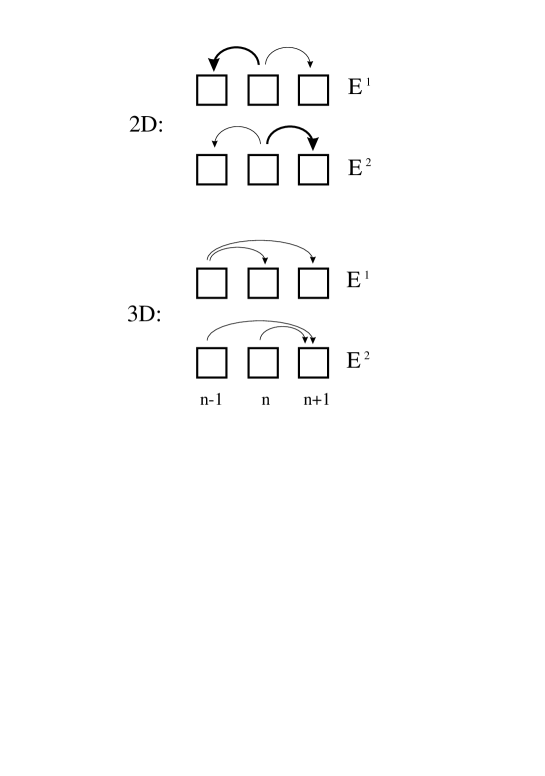
FIG. 2.: The shell triad interactions. Arrows indicates transfer of energy, $E^{1}$, and enstrophy, $E^{2}$, for the 2D case, $\epsilon=5/4$, and energy, $E^{1}$, and helicity, $E^{2}$, for 3D, $\epsilon=1/2$, case. The thickness of the arrows indicates the strength of the transfer.

FIG. 3.: The mean value of the shell velocities as a function of shell number on a logarithmic scale (base $\lambda$), for the 2D case, $\epsilon=5/4,k_{0}=\lambda^{-4},\lambda=2,n=30,\nu=10^{-16},f_{n}=5\times 10^{-3}\times(1+i)\delta_{n,4}$. The model was run for $4.2\times 10^{4}$ time-units.

FIG. 4.: The mean values of, (a), the energy flux, $\Pi_{1}$, and (b) the enstrophy flux, $\Pi_{2}$.

FIG. 5.: Same as figure 3, but with $n=30,\nu=f=0$. Diamonds corresponds to an initial spectral slope of -1.0, that is a high value of A/B. The corresponding curve is statistical equilibrium distribution for $A/B=10^{2}$. Triangles corresponds to an initial spectral slope of -0.8, that is a lower value of A/B. The curve is statistical equilibrium distribution for $A/B=10^{-2}$.

FIG. 6.: The spectral slope $\gamma$ as function of $\epsilon$. The horizontal dashed line is the Kolmogorov scaling for energy cascade. The full curve is the scaling exponent for the enstrophy (or in 3D like case helicity) cascade, and the dotted curve corresponds to the enstrophy (helicity) equipartitioning. All the 3D like models shows energy cascade (equipartitioning corresponds to the line $\gamma=0$). The bold line piece, $0<\epsilon<0.39...$, represents parameter values where the Kolmogorov fixed point is stable [6]. The diamonds are model run with $n=50,k_{0}=\lambda^{-4},\lambda=2,f_{n}=5\times 10^{-4}\times(1+i)\delta_{n,15},(\epsilon=11/10,\nu=5\times 10^{-27},\nu^{\prime}=100),(\epsilon=117/100,\nu=5\times 10^{-27},\nu^{\prime}=100),(\epsilon=5/4,\nu=5\times 10^{-25},\nu^{\prime}=100),(\epsilon=3/2,\nu=5\times 10^{-23},\nu^{\prime}=100),(\epsilon=7/4,\nu=5\times 10^{-23},\nu^{\prime}=100),(\epsilon=2,\nu=5\times 10^{-20},\nu^{\prime}=100).$ The stars are model runs with $n=19,k_{0}=\lambda^{-4},\lambda=2,f_{n}=10^{-4}\times(1+i)\delta_{n,4},\nu=10^{-6},\nu^{\prime}=0,\epsilon=1/2,6/10,7/10$. The 3D like models shows Kolmogorov scaling, with deviations due to intermittency corrections, and energy cascading. The 2D like models shows a cross-over at $\epsilon=5/4$ between statistical equilibrium, $1<\epsilon<5/4$, and enstrophy cascading, $5/4<\epsilon<2$.

FIG. 7.: Same as figures 3 and 4 for $\epsilon=11/10,5/4,3/2,7/4,2$. The spectral slopes are shown in figure 6 (diamonds).

FIG. 8.: Time evolution of shell velocities in the beginning and the end of the inertial subrange. The typical timescale of shell $n$ scales as $T_{n}\sim(k_{n}|u_{n}|)^{-1}\sim k_{n}^{\gamma-1}$. Note that for $\epsilon=5/4$ the timescale is the same for all shells.

FIG. 9.: Probability density functions for real and imaginary parts of shell velocities. The curves are gaussians with the same variance.

FIG. 10.: The deviation of the structure function from Kolmogorov scaling for $\epsilon=11/10,5/4,3/2,7/4,2$.

FIG. 11.: (a) Numerical values of $\delta\zeta(10)$ as a function of $\epsilon$, the error bars represents one standard deviation. (b) Ratio of typical timescales between dissipation scale and forcing scale, $log_{2}(T_{\nu}/T_{f})$ as a function of $\epsilon$. The vertical line indicates the crossover between statistical equilibrium and cascading.

REFERENCES

- [1] E. B. Gledzer, Sov. Phys. Dokl, 18, 216 (1973).
- [2] M. Yamada and K. Okhitani, J. Phys. Soc. of Japan 56, 4210 (1987); Progr. Theo. Phys. 79, 1265 (1988).
- [3] L. Kadanoff, D. Lohse, J. Wang and R. Benzi, Phys. Fluids 7, (1995).
- [4] E. Aurell, G. Boffetta, A. Crisanti, P. Frick, G. Paladin and A. Vulpiani, Phys. Rev. E, 50, 4705, (1994).
- [5] P. Frick and E. Aurell, Europhys. Lett. 24, 725, (1993).
- [6] L. Biferale, A. Lambert, R. Lima, G. Paladin, Physica D, 80, 105 (1995).
- [7] P. D. Ditlevsen, to be published
- [8] M. Yamada and K. Okhitani,Phys. Rev. Lett. 60,983 (1988)
- [9] N. Schörghofer, L. Kadanoff and D. Lohse, preprint 1995.
- [10] R. H. Kraichnan and D. Montgomery, Rep. Prog. Phys., 43, 547, (1980).
- [11] R. H. Kraichnan, J. Fluid Mech., 47, 525, (1971).
- [12] M. H. Jensen, G. Paladin and A. Vulpiani, Phys. Rev. A, 43, 798, (1991).
- [13] O. Gat, I. Procaccia and R. Zeitak, sl preprint, 1994