Phase slips and phase synchronization of coupled oscillators

Abstract

The behaviors of coupled oscillators, each of which has periodic motion with random natural frequency in the absence of coupling, are investigated. Some novel collective phenomena are revealed. At the onset of instability of the phase-locking state, simultaneous phase slips of all oscillators and quantized phase shifts in these phase slips are observed. By increasing the coupling, a bifurcation tree from high-dimensional quasiperiodicity to chaos to quasiperiodicity and periodicity is found. Different orders of phase synchronizations of chaotic oscillators and chaotic clusters play the key role for constructing this tree structure.

The investigation of coupled oscillators has attracted constant interest for many decades [1]. The rich collective behaviors of these systems, such as mutual entrainment, self-synchronization, and so on, are observed in many fields, e.g., coupled laser systems, Josephson junction arrays, biological and chemical oscillators etc. [2-10]. In early studies, interest was focused on coupled oscillators, of which each is periodic without coupling. Recently, the investigation has been extended to coupled chaotic systems (i.e., individual systems are chaotic without coupling). Significant phenomena were found, such as phase synchronization of two mutually coupled chaotic oscillators [11, 12], and clustering and cluster-cluster synchronization of multiple coupled chaotic units for local [13] and global [14] couplings.

In this letter, we study the following $N$ coupled oscillators with the nearest coupling,

$$\stackrel{{\scriptstyle.}}{{\theta}}_{i}=\omega_{i}+\frac{K}{3}[\sin(\theta_{i+1}-\theta_{i})+\sin(\theta_{i-1}-\theta_{i})],$$ (1)

$i=1,2,...,N$, where $K$, $\theta_{i}$ and $\omega_{i}$ are the coupling strength, the angle of modulo $2\pi$ and the natural frequency of the $i$-th oscillator, respectively. Model (1) has been extensively investigated in the past several decades. Here we concentrate on the dynamical behavior of the system. In particular, we are interested in the characteristic features of the motions of individual oscillators, i.e., the microscopic motions, in the regime of desynchronization of the phase-locking state, which have not yet been well investigated by the previous works. Several novel features of this system are found. First, we find simultaneous phase slips of all oscillators at the onset of desynchronization of the phase locking state, and quantized phase shifts in these slips are observed. Moreover, we find the interesting cascade behavior of coupling-induced chaos and a nice tree structure of transitions from qausiperiodicity to chaos to qausiperiodicity and periodicity. Then rich behaviors of synchronizations between chaotic oscillators and chaotic clusters, which have attracted much attention recently for the coupled Rossler and Lorenz oscillators, can be also identified for the rather old as well as popular system (1), of which the individual oscillators have simple periodic motions without coupling. These findings greatly enlarge the application perspectives of chaos synchronization. These features of phase dynamics are expected to be observable in practical systems by experiments, such as coupled laser arrays, Josephson junction chains and coupled electrical circuits.

In Eq. (1) the periodic boundary condition $\theta_{i+N}(t)=\theta_{i}(t)$ is applied. Without losing generality we scale $\omega_{i}$ such that

$$\sum\limits_{i=1}^{N}\omega_{i}=0.$$ (2)

It is well known that for a given $N$ and $\{\omega_{i},\ i=1,...N\}$, there is a critical coupling $K=K_{c}$. For $K>K_{c}$, phase-locking can be observed, and then we have $\{\stackrel{{\scriptstyle.}}{{\theta}}_{i}=0,\ i=1,...,N\}$ , and each $\theta_{i}$ is locked to a fixed value. For $K<K_{c}$, no phase-locking exists, and $\stackrel{{\scriptstyle.}}{{\theta}}_{i}(t)$ are no longer zero. In [8-10], it is found that if we define an average frequency as

$$\stackrel{{\scriptstyle\_}}{{\omega}}_{i}=\lim_{T\rightarrow\infty}\frac{1}{T}\int_{0}^{T}\stackrel{{\scriptstyle.}}{{\theta}}_{i}(t)dt,$$ (3)

synchronization between different oscillators, in the sense of $\stackrel{{\scriptstyle\_}}{{\omega}}_{i}=\stackrel{{\scriptstyle\_}}{{\omega}}_{j}$, $i\neq j$, can be observed in the region where strict phase-locking of $\stackrel{{\scriptstyle.}}{{\theta}}_{i}=0$ is broken. It is interesting to investigate how the various oscillators are led to complete synchronization (phase-locking for $K>K_{c}$) via a sequence of bifurcations by increasing the coupling $K$ from $K=0$.

In order to get a general idea about the global behavior of the system, we first measure the following two positive macroscopic quantities $R$ and $\Omega$:

$$R=\frac{1}{N}\left|\sum\limits_{j=1}^{N}e^{i\theta_{j}}\right|,\quad\Omega=\lim_{T\rightarrow\infty}\frac{1}{T}\int_{0}^{T}{\sum\limits_{i=1}^{N}}\left|\stackrel{{\scriptstyle.}}{{\theta}}_{i}(t)\right|dt.$$ (4)

It is clear that $R$ is time-dependent beyond the phase-locking region. Then we further measure its time average as an order parameter:

$$\left<R\right>=\lim_{T\rightarrow\infty}\frac{1}{T}\int_{0}^{T}R(t)dt,$$ (5)

In Figs. 1(a) and (c), we plot $\Omega$ vs. $K$ for $N=5$ and $15$, respectively. In both cases, natural frequencies are randomly chosen from a normal Gaussian distribution. The actual frequencies can be seen in Fig. 3(a) for $N=5$ and Fig. 3(b) for $N=15$ at $K=0$, respectively. These natural frequencies are used for all figures in this letter. We found, for the given natural frequencies, $K_{c}=5.08$ for $N=5$ and $K_{c}=6.22$ for $N=15$. When $K>K_{c}$ we have identically $\Omega=0$, and then complete synchronization (phase-locking) is justified. In Figs.1(b) and (d) we do the same as (a) and (c), respectively, with the measured quantity replaced by $<R>$. In computing Figs.1, initial conditions of $\theta_{j}(0)$ are randomly chosen, and then in the shaded region of Fig. 1(d) the coexistence of multiple attractors of phase-locking states is justified for $K>K_{c}$. In Fig.1, the quantity $T$ in Eqs. (4) and (5) is taken sufficiently long in our simulations so that the fluctuations due to finite $T$ are invisible. It is interesting to observe that several discontinuities appear in the region $K<K_{c}$, indicating that, apart from the apparent phase-locking transition, some additional transitions exist even before $K_{c}$.

For the microscopic quantities, it is natural to study the velocities of various oscillators. In Figs. 2(a) and (b), we present the motions of $\stackrel{{\scriptstyle.}}{{\theta}}_{i}$ vs. $t$ for $N=5$ and different $K$’s. For $K=0$, $\stackrel{{\scriptstyle.}}{{\theta}}_{i}$ must be equal to the constant $\omega_{i}$, and for small $K$ [see (a)] $\stackrel{{\scriptstyle.}}{{\theta}}_{i}$ varies oscillatorily around its natural frequency. As $K$ increases, the oscillations of $\stackrel{{\scriptstyle.}}{{\theta}}_{i}$ become large, and the oscillation centers of all oscillators shift close to each other. An interesting feature is that near the onset of synchronization [see (b)], we can find simultaneous phase slips, i.e., all oscillators keep in a the phase-locking condition (OFF-state) for a long time, and then simultaneous bursts of all oscillators (ON-state) break the locking state. After a short firings all oscillators calm down again simultaneously to another phase-locking state, and then repeat the same process periodically. As $K$ gets closer to $K_{c}$, the length of the OFF state $\tau$ becomes longer. We find a clear scaling between $\tau$ and $K_{c}-K$:

$$\tau\propto(K_{c}-K)^{-0.5}.$$ (6)

The above features of synchronized actions of phase slips can be well understood by an intuitive explanation. Suppose various oscillators can be locked to a set of phases $\stackrel{{\scriptstyle\_}}{{\theta}}_{i}(K)$ for $K\geq K_{c}$. Then all solutions satisfying

$$\stackrel{{\scriptstyle\_}}{{\theta}}_{i+1}(K,{\bf m})-\stackrel{{\scriptstyle\_}}{{\theta}}_{i}(K,{\bf m})=\stackrel{{\scriptstyle\_}}{{\theta}}_{i+1}(K)-\stackrel{{\scriptstyle\_}}{{\theta}}_{i}(K)+2\pi m_{i}$$ (7)

with ${\bf m}=(m_{1},...,m_{j},...m_{N})$ and $m_{i}$ being any integer, must also be phase-locking solutions of (1). By reducing $K$ lower than $K_{c}$, all the above solutions lose their stability via the saddle-node bifurcation. At $K=K_{c}$, there exists a heteroclinic path linking some of the above solutions, which has the lowest potential, and is attracting (the existence of such a heteroclinic path can be rigorously proven for $N=2$). For $K<K_{c}$, and $\left|K-K_{c}\right|\ll 1$, the system takes such a periodic path, which stays in the vicinity of one of the above stationary solution for a long time, and escapes away from this solution (simultaneous phase slips for all oscillators), and then approaches to the vicinity of the next stationary solution alone the heteroclinic path of $K=K_{c}$; this produces the periodic pulses of Fig. 2(b). The scaling property of time length of the OFF-state $\tau$ can be also computed since for the saddle-node bifurcation we have a universal form $\stackrel{{\scriptstyle.}}{{x}}=(K_{c}-K)+x^{2}.$ The time $\tau$ for $x$ to move from $x=0$ to $x\rightarrow\infty$ reads $\tau\propto\int_{0}^{\infty}\frac{dx}{(K_{c}-K)+x^{2}}=\frac{\pi}{2\sqrt{K_{c}-K}}$; this explains our observation of the scaling law of Eq. (6).

It is interesting to compute the phase shifts for various oscillators in each phase slip pulse in Figs. 2(b). Let $\Delta\theta_{i}$ represent the phase shift of $\theta_{i}$ during each pulse. From (1) and (2) we have

$${\sum\limits_{i=1}^{N}\Delta\theta_{i}=0.}$$ (8)

We argue that any two adjacent fixed points in a heteroclinic path at $K=K_{c}$ take $m_{i}=0$ or $\pm 1$ in Eqs. (7), i.e.,

$$\Delta\theta_{i+1}-\Delta\theta_{i}=0\text{ or }\pm 2\pi$$ (9)

for $i=1,...,N-1$. Considering both conditions (8) and (9), $\Delta\theta_{i}$ can take only quantized values

$$\Delta\theta_{i}=0,\pm\frac{2\pi}{N},\pm\frac{4\pi}{N},...,\pm\frac{2(N-1)\pi}{N},\pm 2\pi.$$ (10)

The concrete value for each $\Delta\theta_{i}$ depends on the particular distribution of $\omega_{i}$. In Figs.2(c) and (d) the phase shifts observed in all pulses fully agree with our heuristic argument. Further considering Fig.3, the phase shifts in Fig.2 can be exactly predicted (see [15]). One more conclusion from the above analysis is that at the onset of instability of the phase-locking state, all velocities $\stackrel{{\scriptstyle\_}}{{\omega}}_{j}$ have the scaling $\stackrel{{\scriptstyle\_}}{{\omega}}_{j}\propto\sqrt{K_{c}-K}$, and the ratios between different $\stackrel{{\scriptstyle\_}}{{\omega}}_{j}$ must be quantized to discrete rational numbers.

As we further reduce $K$ to values considerably smaller than $K_{c}$, no more phase-locking exists, and no apparent synchronization can be observed directly for $\stackrel{{\scriptstyle.}}{{\theta}}_{j}(t)$. However, some other implicit synchronization — phase synchronization — can be still found. To get a general idea, we plot $\stackrel{{\scriptstyle\_}}{{\omega}}_{i}$ defined in (3) vs. $K$ for $N=5$ and $15$ in Fig. 3(a) and (b), respectively, by varying $K$ from $K=0$ to $K>K_{c}$. Interesting behavior of transition tree for phase synchronization is clearly shown. Though some synchronizations can be expected from the observations of frequency plateaus reported in previous papers [8-10], a number of characteristic features revealed in these trees are novel and interesting. Three kinds of transitions can be observed in these trees. First, if two adjacent oscillators (or adjacent clusters of oscillators) have close frequencies, they can be easily synchronized by increasing $K$. In this case, one always finds two branches merging to a single one (indicated by A). Second, if two non-adjacent oscillators (or two non-adjacent clusters) have close frequencies while the oscillators between them have considerably different frequencies, one can find the non-adjacent oscillators can be also synchronized to each other, i.e., non-local clusters can be formed, and these non-local clusters can quickly bring the oscillators between them to the synchronized status, and form a solidly larger synchronized cluster. In this case, the transition may be from two to one or from multiple branches to one (indicated by B). An oscillator, which is synchronized to a cluster for certain $K$, can be desynchronized from the original cluster by increasing $K$. This desynchronization always happens at an edge oscillator of a cluster, due to the competition between two neighbor clusters (indicated by C, see 2nd and 3rd oscillators of Fig. 3(b)). It is obvious that C is the inverse of A. The transitions of types B and C have never been realized before.

The most interesting and novel finding is the nature of these synchronizations. The motions in these synchronization trees may be very different. They can be periodic, quasiperiodic and chaotic. In Fig. 4(a), we take $N=15$ and plot the largest Lyapunov exponent of the system vs. $K$. In a large interval of $K$, we find the positive Lyapunov exponent, indicating chaos. Thus, in this region phase synchronizations of chaotic oscillators are identified. Recently, the phase synchronization of coupled chaotic systems has attracted great attention [11]. Here the major difference between our system and the previous chaos synchronization is that our oscillators are periodic without coupling, and chaos is induced by the coupling, while in the latter case the individual systems are chaotic without coupling. Moreover, we find that these coupling-induced chaotic motions of different oscillators may have different levels of synchronizations by varying the coupling, and the cascade of synchronization forms a tree-like structure of Fig. 3.

In Figs. 4(b) to (f) we plot the maps of $\stackrel{{\scriptstyle.}}{{\theta}}_{1}(n)$ to $\stackrel{{\scriptstyle.}}{{\theta}}_{1}(n+1)$, where $\stackrel{{\scriptstyle.}}{{\theta}}_{1}(n)$ is the $\stackrel{{\scriptstyle.}}{{\theta}}_{1}$ value at the time $t$ when $\theta_{1}(t)$ crosses the angles $2n\pi$ with $n$ being an integer. For $K>K_{c}$, we have fixed point solution, and the map is fixed at $\stackrel{{\scriptstyle.}}{{\theta}}_{1}(n)=\stackrel{{\scriptstyle.}}{{\theta}}_{1}(n+1)=0$. For $K$ slightly smaller than $K_{c}$ we have periodic solution represented by the finite number of dots in Fig. 4(b). The period $8$ can be easily understood from Fig. 2(d). The period of the total system is $15\tau$, where $\tau$ is the time interval between the two adjacent slips, and the change of of $\theta_{1}$ in $15\tau$ is $-16\pi$. This leads to the period-$8$ solution of Fig. 4(b). Two-frequency torus can be identified in the three-cluster regime [see Fig. 4(c)]. For very small $K$, we can find high-dimensional quasiperiodicity [e.g., Fig. 4(f)]. Chaos is prevailing in the $K$ region between Fig. 4(c) and 4(f) [see Fig. 4(d) and (e), and Fig. 4(a)]. Many periodic windows are found in the quasiperiodic and chaotic regions, which will be investigated in detail in our forthcoming extended paper.

The entire variation from high-dimensional quasiperiodicity (for very small $K$) to periodic motion ($K<K_{c}$, $\left|K-K_{c}\right|\ll 1$) through various orders of chaos synchronizations can be vitally seen in Figs. 3 and 4. Starting from the high-dimensional quasiperiodicity for $K\ll 1$, by increasing $K$ various neighboring oscillators with close frequencies start to form clusters via phase synchronization, and chaos is induced near the first synchronization. Then in each cluster, different oscillators perform different chaotic motions, while having identical winding number. The winding numbers for different chaotic clusters are different. When further increasing $K$, adjacent chaotic clusters can be synchronized to form larger clusters, until two large clusters are formed when the motion becomes periodic. This tree picture of the transitions is expected to be the same for general large number of coupled non-identical oscillators, which are periodic in bare case.

Since system (1) qualitatively describes practical situations in wide fields, ranging from physics, chemistry to biology, the findings in this letter are expected to be of general significance, and they can be used for understanding the mechanisms of rich collective behaviors of coupled systems. Laser arrays, Josephson junction chains and coupled electrical circuits may be ideal candidates for experimentally revealing the features explored in this letter.

This work is supported in part by the Research Grant Council RGC and the Hong Kong Baptist University Faculty Research Grant FRG and in part by the National Natural Science Foundation of China.

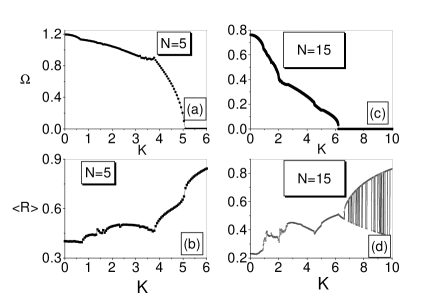
FIG. 1.: $\Omega$ and $<R>$ defined in Eqs. (4) and (5) plotted vs. $K$ for $N=5$ and $15$. The natural frequencies are shown in Fig. 3 at $K=0$. $K_{c}=5.08$ and $6.22$ for $N=15$ and $N=15$. For $K>K_{c}$, phase-locking can be observed, and the shaded region in (d) indicates the coexistence of multiple attractors of phase-locking states. Initial conditions are randomly chosen for each $K$ detected.

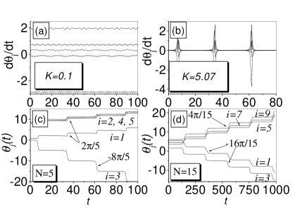
FIG. 2.: (a), (b): The time evolutions of $\stackrel{{\scriptstyle.}}{{\theta}}_{i}$ plotted for $N=5$ and two different $K$. Near the onset of the instability of the phase-locking state [(b)], simultaneous phase slips of all oscillators are clearly seen. (c), (d): Some $\theta_{i}(t)$ plotted against $t$ near $K_{c}$. (c) $K=5.07$, $N=5$; (d) $K=6.212$, $N=15$. Quantization of phase shifts for all oscillators at each phase slip and the pulse are justified.

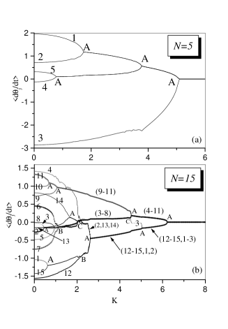
FIG. 3.: Transition trees of synchronization for averaged velocities versus $K$. (a) $N=5$, (b) $N=15.$ Note the existence of three kinds of transitions labeled by A, B and C.

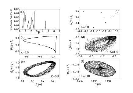
FIG. 4.: (a) The largest Lyapunov exponent of the coupled oscillators plotted against $K$, $N=15$. (b)-(f) give the maps of $\stackrel{{\scriptstyle.}}{{\theta}}_{1}(n+1)$ vs. $\stackrel{{\scriptstyle.}}{{\theta}}_{1}(n)$ where $\stackrel{{\scriptstyle.}}{{\theta}}_{1}(n)$ is the value of $\stackrel{{\scriptstyle.}}{{\theta}}_{1}(t)$ when $\theta_{1}$ crosses $2\pi n$. (b) $K=6.0$, the motion is periodic. (c) $K=3.0$, the motion is quasiperiodic with two irreducible frequencies. (d), (e): $K=1.5$ and $0.9$, respectively. The motions are chaotic. (f) $K=0.01$, the motion is high-dimensional quasiperiodicity.

REFERENCES

- [1] H. Haken, Advanced Synergetics (Springer, Berlin, 1983).
- [2] Y. Kuramoto, Chemical Oscillations, Waves, and Turbulence (Springer, Berlin, 1984); A. T. Winfree, The geometry of Biological Time (Springer, Berlin, 1980).
- [3] A. H. Cohen, P. J. Holmes and R. H. Rand, J. Math. Biology 13, 345 (1982); G. B. Ermentrout, J. Math. Biology 23, 55 (1985).
- [4] K. Wiesenfeld, P. Colet and S. H. Strogatz, Phys. Rev. Lett. 76, 404 (1996).
- [5] S. H. Strogatz, R. E. Mirollo and P. C. Matthews, Phys. Rev. Lett. 68, 2730 (1992); H. Daido, Phys. Rev. Lett. 61, 231 (1988).
- [6] H. Tanaka, A. J. Lichtenberg and S. Oishi, Phys. Rev. Lett. 78, 2104 (1997).
- [7] P. Tass, Phys. Rev. E 56, 2043 (1997); T. W. Carr and I. B. Schwartz, Physica D 115, 321 (1998).
- [8] H. Sakaguchi, S. Shinomoto and Y. Kuramoto, Prog. Theor. Phys. 77, 1005 (1987); 79, 1069 (1988).
- [9] S. H. Strogatz and R. E. Mirollo, J. Phys. A 21, L699 (1988); Physica D 31, 143 (1988); N. Kopell and G. B. Ermentrout, Commun. Pure Appl. Math. 39, 632 (1986).
- [10] J. L. Rogers and L. T. Wille, Phys. Rev. E 54, R2193 (1996).
- [11] M. Rosenblum, A. S. Pikovsky and J. Kurths, Phys. Rev. Lett. 76, 1804 (1996); 78, 4193 (1997).
- [12] E. J. Rosa, E. Ott, and M. H. Hess, Phys. Rev. Lett. 80, 1642 (1998).
- [13] G. V. Osipov, A. S. Pikovsky, M. G. Rosenblum, and J. Kurths, Phys. Rev. Lett. E 55, 2353 (1997).
- [14] A. S. Pikovsky, M. G. Rosenblum and J. Kurths, Europhys. Lett. 34, 165 (1996).
- [15] From Fig.3(a) and Eqs.(7) and (8), we have and which lead to , and , . The same computation from Fig. 3(b) leads to , , producing for and for .