Delayed Dynamics toward Applications

Abstract

We propose two dynamical models with delay taking advantage of their complex dynamics for information processing tasks. The first model incorporates coupled delayed dynamics of multiple bits, which is shown to have desirable properties as an encryption scheme. The second model is a single binary element with delayed stochastic transition, which presents a resonance behavior between noise and delay.

1 INTRODUCTION

Complex behaviors due to time delays are found in many natural and artificial systems. Some examples are delays in bio-physiological controls [1, 2], and signal transmission delays in large–scale networked or distributed information systems (See e.g. [3, 4]). Research on systems or models with delay has also been carried out in the fields of mathematics [5, 6], artificial neural networks [7, 8], and in physics [9, 10, 11]. This series of research has revealed that time delay can introduce surprisingly complex behaviors to otherwise simple systems, because of which delay has been considered an obstacle from the point of view of information processing.

In this paper, however, we actually take advantage of this complexity with delayed dynamics and propose two models. The first model incorporate delayed dynamics into a new model of encryption. The second model shows a resonance behavior between noise and delay. Through these two models, we explore the possibility of applications for delayed dynamics.

2 THE ENCRYPTION MODEL

The encryption process is identified with a coupling dynamics with various time delays between different bits in the original data. We show that the model produces a complex behavior with the characteristics needed for an encryption scheme.

Let us now describe the encryption model in more detail. ${\bf{S}}(0)$ is the original data of $N$ binary bits, whose $i$th element $s_{i}(0)$ takes values $+1$ or $-1$. The delayed dynamics for the encryption can be specified by a key which consists of the following three parts: (1) a permutation ${\bf P}$ generated from $(1,2,3,..,N)$, (2) a delay parameter vector $\tau$ which consists of $N$ positive integers, and (3) number of iterations of the dynamics $T$. Given the key $K=({\bf P}$, $\tau$, $T)$, the dynamics is defined as

$$s_{i}(t)=(-1)\times s_{p_{i}}(t-\tau_{i}),$$ (1)

where $p_{i}$ and $\tau_{i}$ are $i$th element of ${\bf P}$ and $\tau$, respectively. (If $t-\tau_{i}<0$, we set $t-\tau_{i}=0$.) In Figure 1, this dynamics is shown schematically. The state of the $i$th element of ${\bf{S}}(t)$ is given by flipping the state of the $p_{i}$th element of ${\bf{S}}(t-\tau_{i})$. Thus this dynamics causes interaction between $N$ bits of the data in both space and time. The encoded state ${\bf{S}}(T)$ is obtained by applying this operation of equation (1) iteratively $T$ times starting from ${\bf{S}}(0)$.

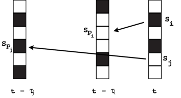
Figure 1: Schematic view of the model dynamics. The state of the $i$th element of ${\bf{S}}(t)$ is given by flipping the state of the $p_{i}$th element of ${\bf{S}}(t-\tau_{i})$.

We investigate numerically the nature of the delayed dynamics from the perspective of measuring the strength as an encryption scheme. First, we examine how the state ${\bf{S}}(t)$ evolves with time. In Figure 2 (A), we have shown an example of encoded states with different $T$ using the same ${\bf P}$ and $\tau$ for a case of $N=81$. To be more quantitative, we compute the following quantity as a measure of difference between two encoded states at different times $t$ and $t_{f}$:

$$Y(t)={1\over N}\,\sum_{i=0}^{N}S_{i}(t)S_{i}\left(t_{f}\right)$$ (2)

A typical example is shown in Figure 2(B). We note that the dynamics of our model has a property of occasionally very similar, but not exactly the same, states appearing indicated by sharp peaks in the figure. Except around these particular points, however, we generally obtain rather uncorrelated encoded states (i.e., $Y\approx 0$) with different iteration times. This is a desirable property of the model as an encryption scheme: the same state can be encoded into uncorrelated states by changing $T$.

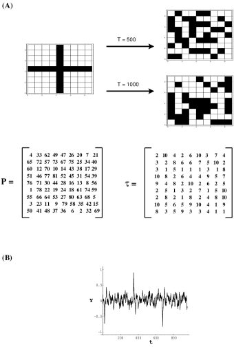
Figure 2: (A) Examples of encoding with the model dynamics from an initial state to $T=500$ and $T=1000$ with ${\bf P}$ and $\tau$. (B) Example of the correlation $Y$ between encoded states at different time steps evaluated by equation (2). Cases with $t_{f}=1000$ are plotted with the initial state and ${\bf P}$ and $\tau$ the same as in Figure 2 (A).

Next, we investigated the effect of a minor change of ${\bf P}$ and $\tau$ on the model dynamics. Starting with the same initial condition, we evaluate how two states ${\bf{S}}(t)$ and ${\bf{S^{\prime}}}(t)$ are encoded with slightly different ${\bf P}$ and ${\bf P^{\prime}}$, respectively, by computing

$$X(t)={1\over N}\,\sum_{i=0}^{N}S^{\prime}_{i}(t)S_{i}\left(t\right)$$ (3)

A representative result is shown in Figure 3(A). The same evaluation with $\tau$ and $\tau^{\prime}$ is shown in Figure 3(B). These graphs indicate that if we take sufficiently large $T$, the same state can evolve into rather uncorrelated states with only a slight change of ${\bf P}$ and $\tau$. This again is a favorable property in the light of encryption. It makes iterative and gradual guessing of ${\bf P}$ and $\tau$ in terms of their parts and elements very difficult: a nearly correct guess of the values of ${\bf P}$ and $\tau$ does not help in decoding.

Figure 3: Example of the correlation $X$ evaluated by equation (3) between two states encoded by slightly different (A) ${\bf P}$ and ${\bf P^{\prime}}$, and (B) $\tau$ and $\tau^{\prime}$. The difference of ${\bf P^{\prime}}$ from ${\bf P}$, and $\tau^{\prime}$ from $\tau$ are indicated by boxes. The initial state and ${\bf P}$ and $\tau$ are the same as in Figure 2.

With these properties of the model, an exhaustive search appears to be the only method for guessing the key. Even if one knows $N$ and $\tau_{max}$, the largest element in $\tau$, one is still required to search for the correct key from among $(N!)(\tau_{max})^{N}$ combinations and to guess $T$. The commonly used DES (Data Encryption Standard) employs $2^{56}$ bit keys [12]. We can obtain a similar order of difficulty with rather small values of $N$ and $\tau_{max}$; for instance, $N\approx 11$ and $\tau_{max}\approx 10$ [13].

There are different methods possible for using this model for a secure communication between two persons who share the key. One example is that the sender sends a series of encoded data in sequence for the interval between $T$ and $T+\tau_{max}$ (or longer). The receiver can recover the original data from this set of encoded data by applying a reverse dynamics with the key. In a situation where the data sent is a choice out of multiple data sets known to the receiver, the receiver can run the encryption dynamics to the entire sets with the key for case matching.

3 RESONANCE BETWEEN NOISE AND DELAY

The second model is a stochastic binary element with delayed transition which is schematically shown in Figure 4. The state of the element $X(t)$ at time step $t$ can take either $-1$ or $1$ and the transition probabilities are indicated by the arrows. We further include delay in the model, which makes the formal definition of the model as follows:

$$P(1,t+1) = p\ \ \quad X(t-\tau)=-1,$$ (4)

$$= 1-q\quad X(t-\tau)=1,$$

$$P(-1,t+1) = q\ \ \quad X(t-\tau)=1,$$ (5)

$$= 1-p\quad X(t-\tau)=-1,$$

where $P(s,t)$ is a probability that $X(t)=s$.

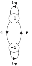
Figure 4: Schematic view of the stochastic model dynamics.

Hence, the transition probability of this model depends on its state at $\tau$ steps earlier. In this sense, this model is a special case of ”delayed random walks”[11, 14] except it can take only two states.

Let us now discuss our motivation for considering such a model. It has been shown that a simple stochastic binary element can show a resonant behavior with a external oscillating signal with an appropriate choice of transition probability. This phenomena is termed as “Stochastic Resonanc” (see e.g. [15]) now widely investigated. In our model here, we have replaced an external oscillatory signal with delay and its associated oscillatory behavior. Hence, we can expect some form of resonance can be seen with the model between the oscillatory dynamics due to noise and that due to delay.

A preliminary simulation study shows this is indeed the case. We have fixed $q=1-q=0.5$ and $\tau=10$, and varied $p$. The simulations are done up to 20000 steps. In Figure 5, where we have plotted examples of residence time histograms in the $-1$ state and dynamics of $X(t)$, we can see a resonance phenomena as a height of the peak at the period equal to the delay. If we tune the noise ($p$) appropriately, we observe the height of the residence time histogram peak reaching the maximum value. This is shown in Figure 6[16].

With this property, this model can be used to stochastically encode information. We have built a preliminary application to encode static pictures using this model, which will be reported elsewhere.

4 Summary

We have proposed two models which include delay. These two models indicate that complex delayed dynamics can be used for information processing tasks rather than necessarily being obstacle. More thorough investigation of each model is presented elsewhere, and concrete applications of these models are currently being devloped.

Figure 5: The residence time histogram and dynamics of $X(t)$ as we change $p$. The values of $p$ are (A) $p=0.005$, (B) $p=0.04$, (C) $p=0.2$.

Figure 6: A plot of peak height with varying $p$

References

- [1] M. C. Mackey and L. Glass, Science 197, 287 (1977);
- [2] A. Longtin and J. Milton, Biol. Cybern. 61, 51 (1989);
- [3] P. Jalote, Fault Tolerance in Distributed Systems. (Prentice Hall, NJ, 1994).
- [4] N. K. Jha and S. J. Wang, Testing and Reliable Design of CMOS Circuits. (Kluwer, Nowell, MA, 1991).
- [5] K.L. Cooke and Z.Grossman, J. Math. Analysis and Applications 86, 592 (1982);
- [6] U. Küchler and B. Mensch, Stochastics and Stochastics Reports 40, 23 (1992).
- [7] C. M. Marcus and R. M. Westervelt, Phys. Rev. A 39, 347 (1989);
- [8] J. A. Hertz, A. Krogh, and R. G. Palmer, Introduction to the Theory of Neural Computation (Addison–Wesley, Redwood City, CA, 1991).
- [9] M. W. Derstine, H. M. Gibbs, F. A. Hopf and D. L. Kaplan. Phys. Rev. A 26, 3720 (1982);
- [10] K. Pyragas. Phys. Lett. A 170, 421 (1992);
- [11] T. Ohira, Phys. Rev. E 55, R1255 (1997).
- [12] For description of DES, see e.g., A. J. Menezes, P. van Oorschot, and S. A. Vanstone, Handbook of Applied Cryptography (CRC Press, 1996). A bit key scheme was recently revealed in an open challenge using many computers over the Internet. (http://www.rsa.com/pressbox/html/980226.html).
- [13] The search space increases rapidly in particular with the increase of due to factorials.
- [14] T. Ohira and J. G. Milton, Phys. Rev. E.52, 3277, (1995).
- [15] A. R. Bulsara and L. Gammaitoni, Physics Today, 49, 3, 39, (1996).
- [16] For the case of fixed and varying , a preliminary investigation shows that a monotone decreasing histograms appear for .