Chemical or biological activity in open chaotic flows

I Introduction

Active processes taking place in chaotic hydrodynamical flows have attracted recent interest [1]-[10]. By chaotic we mean time-dependent but nonturbulent velocity fields with chaotic tracer dynamics (Lagrangian chaos) [11]-[13]. In the simplest approximation we can assume that the advected particles undergo certain chemical or biological changes but do not modify the fluid flow. The motivation for such studies has been to understand the effects of imperfect mixing [3] due to the underlying chaotic particle dynamics. The implications can be perceived in laboratory experiments [3, 14], but the effects are perhaps more striking in environmental flows. In particular, there is increasing evidence of filamental structures in the product distribution of environmental processes both in the atmosphere, such as ozone reactions [4, 5, 6, 8, 9], and resulting from the interaction of populations of microorganisms in the sea, such as plankton distributions [15, 16]. Our aim is to show that these structures might be consequences of the fractal structures of the reaction free flows [7].

Here we shall consider open flows with asymptotic simplicity in which the velocity field in the far up and downstream regions is uniform. A well-known (time-periodic) laboratory example is the flow around a cylinder. Its actual realization can be observed in environmental flows, like, e.g., in the fluid motion in the wake of a pillar or in the motion of air behind an isolated mountain. A unique feature of such open flows is the pronounced and stable fractal feature associated with the chaotic tracer dynamics [17]-[27], which is clearly measurable in experiments [28]. The central object governing the dynamics is a nonattracting chaotic saddle [29] containing an infinite number of periodic and nonperiodic tracer orbits which remain bounded and never reach either the far up or the downstream regions. A characteristic quantity of the saddle is its escape rate $\kappa$ whose reciprocal value is the average chaotic lifetime. The far up and downstream regions are foliated by the saddle’s stable and unstable manifold, respectively. The saddle’s unstable manifold directs tracers ever approaching the saddle to the far downstream region. Though both the saddle and its manifolds are not space-filling fractal objects, it has been pointed out [17] - [28] that the unstable manifold is the avenue of propagation and transport in such flows. It is the pronounced fractal structure of such flows (which is not present in closed flows) that makes them specially interesting catalyst of active processes [7].

In this paper we consider the advection of active particles in flows with asymptotic simplicity in which the activity is assumed to be of chemical or biological origin in the simplest possible form. The reaction is a kind of “infection” leading to a change of certain properties, such as color of reacting particles. Particles with new properties are the products. Since it is in the close vicinity of the chaotic saddle and its unstable manifold that the particles spend the longest time close to each other, it is there where the effect of the activity is most pronounced. It is then natural to expect that the products should accumulate along the unstable manifold and trace out this fractal object.

In our work we support this conjecture and present a detailed analysis of such active processes. We show that the unstable manifold of the chaotic saddle is the backbone of the reaction. The newly born components cover the branches of the unstable manifold with a well defined average width $\varepsilon^{*}$. Thus, an effective fattening up of the fractal set takes place due to the activity of the tracers. This implies that on linear scales smaller than this width $\varepsilon^{*}$, fractality is washed out, but a clear fractal scaling of the material with a dimension $D_{0}$ can be observed on larger scales. This fractal dimension is the same $D_{0}$ as that of the unstable manifold in the reaction free flow. Although the fractal set itself is a set of measure zero, the amount of chemical products is finite due to the fattening-up process of this manifold.

A consequence of the fractal backbone is that the amount of the reaction product follows a singular scaling law with irrational $D_{0}$-dependent powers of the number of product particles, signaling a singular enhancement of productivity [7]. (The enhancement of activity is meant in comparison with non-chaotic, e.g., stationary flows.) This singularly enhanced rate of activity has profound practical consequences. It may account for the observed filamental patterns of intense activity in environmental flows [4, 5, 6, 8], an effect that cannot be explained if one considers diffusion processes alone. In this work we show how small-scale structures are generated in the dynamics of active particles, and how these dynamical structures are responsible for the enhancement of activity.

In summary, the effect of the chaotic saddle producing this activity is twofold: (i) to keep the reacting particles longer, as given by the escape rate $\kappa$, in the interaction region, and (ii) to generate the unstable manifold’s fractal structure that brings the reacting particles together.

We derive the corresponding reaction equations in the form of maps or differential equations depending on the regime under consideration. Such processes are generalization of classical surface reactions [30], but, by contrast, in our case the surface is a fattened-up fractal. The reaction equations contain new terms not present in the traditional well-stirred reaction model of the same process. In spite of the passive tracers’ Hamiltonian dynamics, these reaction equations turn out to be of dissipative character possessing attractors.

We find that the chemical activity and the advection by the hydrodynamical flow are in permanent competition. Due to this competition, most typically, a kind of stationary state sets in after sufficiently long times. In the case of time-periodic flows of period $T$, the asymptotic state is typically also periodic with $T$, i.e., the reaction becomes synchronized to the flow. Thus, a chaotic particle dynamics is consistent with a non-chaotic reaction dynamics.

To be more specific, we consider simple kinetic models [1] with disk-like particles. Two particles of different kinds undergo a reaction if and only if they come within a distance $\sigma$, which is the interaction range. Due to the incompressibility of the fluid (which is always a good approximation for velocities much below the speed of sound), two-dimensional flows are area-preserving. Therefore, if we cover a layer of fluid by particles, this single-particle coverage of the layer will not change in time. In other words, the average linear distance $\varepsilon_{0}\leq\sigma$ between the actual nearest-neighbor particles is constant. (Note, however, that the linear distance between specific particles is typically increases in time due to the chaotic dynamics.) Thus, the result of the reaction is just the spreading of the products in the layer of particles being advected by the flow. We emphasize again that particles are assumed to have no feedback on the flow. Furthermore, the advection dynamics is purely deterministic, i.e., we work in the limit of weak diffusion where the reaction range represents some kind of diffusion distance too.

We shall consider both an autocatalytic process, $A+B\rightarrow 2B$, and a collisional reaction $A+B\rightarrow 2C$. In both cases $A$ is considered to be the background material which covers initially the full infinite layer of observation. In the autocatalytic process a single seed of particle $B$ is sufficient to trigger reactions leading to the stationary state, while in the collisional reaction a continuous feeding of material $B$ is necessary.

For computational convenience we assume that the reactions are instantaneous and take place at integer multiples of a time lag $\tau$. We shall see that an important dimensionless parameter will be the ratio between the time lag and the average chaotic lifetime: $\nu=\tau/(1/\kappa)=\tau\kappa$. This can also be considered to be the dimensionless reaction time, whose reciprocal value tells us how many reaction events occur on the characteristic time of chaos.

The case of time continuous reactions is obtained in the limit $\tau\rightarrow 0$ (or $\nu\rightarrow 0$) by keeping the reaction front velocity $v_{r}$ finite. In this limit we assume, too, that the average distance $\varepsilon_{0}$ between particles goes also to zero, and we obtain a continuous distribution of particles. We call this limit the chemical frame. A fractal product distribution is then expected to appear if the reaction is slow compared to the flow ($v_{r}\ll\kappa L$ with $L$ as a characteristic length). An example for time continuous reactions is related to the depletion of ozone at the polar vortex: the trimolecular reaction of ClO with NO₂. In late winter and early spring the polar vortex exhibits high concentrations of ClO and very low concentrations of NO₂ while outside the vortex the situation is typically reversed with relatively high concentrations of NO₂ and low concentrations of ClO. Thus the reaction ClO$+$NO${}_{2}\rightarrow$ ClONO₂ is a natural candidate to produce a filamental ClONO₂ distribution along the edge of the polar vortex [5, 8, 9, 31, 32] on the time scale of a few days, where the molecular diffusivity is negligible.

In order to contrast our work with the conventional description of chemical processes, we briefly discuss now the continuous time dynamics of the autocatalytic surface reaction $A+B\rightarrow 2B$ in a uniform flow. Let us observe the flow moving to the right with velocity $v_{0}$ in a unit square (fixed to the observer at rest). A seed particle of type $B$ is kept fixed about the middle of the left boundary. Particles of type $A$ are distributed with uniform density everywhere on the surface of the flow (also upstream). The seed particle starts to interact with its $A$ neighbors transforming them into $B$. Since $B$ particles are transported away, more and more $A$ particles are converted into $B$. Let us assume that at time $t$ the $B$ particles cover a triangle across the square which is symmetric about a horizontal line (Fig. 1).

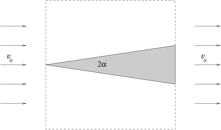
FIG. 1.: Schematic diagram of a uniform flow of velocity $v_{0}$ with autocatalytic reaction. A single seed $B$ is kept fixed at the left corner of the gray triangle occupied by material $B$ which lies in a layer of white $A$ particles. The observation region is a unit square (dashed line).

We assume that the half angle $\alpha$ is small. The area ${\cal A}_{B}$ occupied by $B$ is simply $\alpha$. The change in this area during time $dt$ is due to a horizontal displacement $v_{0}dt$ and a vertical increase $v_{r}dt$ of both fronts, where $v_{r}$ is the reaction front velocity. The gain of the area ${\cal A}_{B}$ is just $2(-v_{0}\alpha+v_{r})dt=$ $2(-v_{0}{\cal A}_{B}+v_{r})dt$. The differential equation governing this area is thus

$$\dot{{\cal A}}_{B}=-2v_{0}{\cal A}_{B}+2v_{r}.$$ (1)

It has a stationary solution, corresponding to a stabilized triangular distribution of $B$ particles of area ${\cal A}_{B}^{*}\equiv\alpha^{*}=v_{r}/v_{0}$. We shall see that the presence of a saddle in a time dependent nonuniform flow results in a slower decay and a faster production ($2v_{0}$ is replaced by the escape rate $\kappa$ and the production term will contain a factor with a negative power of the area itself due to the fractality of the unstable manifold).

For generality, we also investigate cases where the time lag $\tau$ is finite so that its dimensionless version $\nu$ is of order unity or larger. If $\nu$ exceeds a critical value, we find that no product remains, i.e., an emptying transition takes place. Because of the finite values of $\tau$, and the discrete character of the particles ($\varepsilon_{0}$ might also be considered as the size of particles), this latter effect might be of relevance to biological processes accompanying advection. An example can be a crude model of the dynamics of plankton populations [15, 16] in the presence of a time dependent flow. The so-called zooplanktons ($B$) have a daily rhythm: they sink down during night time but come up to the surface of the sea again during day-time when they eat up phytoplanktons ($A$), reproduce themselves and then grow in number.

This paper is organized as follows. In Sec. II, we present the model and the numerical procedure used, while the results for both reaction types are shown in Sec. III. A detailed theory based on these observations is derived in Sec. IV. The concluding Sec. V gives remarks on properties expected to be valid in more general models of active processes in open flows.

II The model flow and numerical procedure

The flow chosen to illustrate the fractal active dynamics is an example of a two-dimensional, incompressible time-periodic fluid motion, the case of the von Kármán vortex street in the wake of a cylinder [18]- [28]. The radius $R$ of the cylinder and the period $T$ of the flow are taken as the length unit and the time unit, respectively. In what follows we keep the flow parameters constant, implying a fixed value of the escape rate $\kappa$, and investigate the dependence of the reaction outcome on parameters like the reaction range ($\sigma$) and time $(\nu)$.

For simplicity, we use an analytic model for the stream function introduced in Ref. [20] (the explicit form of the stream function can also be found in the Sec. III of Ref. [24]). This model has been motivated by direct numerical simulations at Reynolds number of about 250 [19], and has been used successfully to reproduce qualitative features of the tracer dynamics. The escape rate of the particles in the reaction free flow is $\kappa=0.36$ and the fractal dimension of the unstable manifold is $D_{0}=1.61$, while the background flow velocity is $v_{0}=14$ [20, 24].

Since the flow is periodic, we fix the “phase” of the reaction relative to the flow. We consider time zero, $t=0$, to be the instant when a vortex is born close to the surface of the first quadrant of the cylinder and, simultaneously, a fully developed vortex is detaching in the fourth quadrant of the surface [20, 24].

For convenience, we carry out the simulations on a uniform rectangular grid of lattice size $\varepsilon_{0}$ covering both the incoming flow and the mixing region in the wake of the cylinder. This $\varepsilon_{0}$ also corresponds to the average distance between nearest-neighbor particles. If there is a tracer inside a cell, it is always considered to be in its center; the reaction range is bounded from below by the lattice size: $\varepsilon_{0}\leq\sigma$. This projection of the tracer dynamics on a grid essentially defines a mapping among the cells.

The course of the chemical reaction starts with nearly all cells occupied by species $A$, the background material. Few cells contain $B$ distributed according to the initial conditions chosen for the type of reaction under consideration. One iteration of the process just described consists of two mappings in involution. The first mapping models the advection of the particles on the chosen grid, while the second models the instantaneous active process (e.g. chemical reaction) occurring on the same grid of cells. In fact, in any closed region considered there is a loss of the products due to the advection but also a gain in the product amount due to the reaction. Later we find a balance between these two competing effects manifested in a steady state in the product distribution. The simulation consists of a repeated application of advection and reaction steps. We apply different algorithms for different reaction types.

A Autocatalytic reaction: $A+B\rightarrow 2B$

If a tracer starting from the center of a cell is advected into another one after time $\tau$, then the latter cell is considered to be the image of the first one with respect to the dynamics. After an application of the map, a cell will be considered occupied by reagent $B$ if it is an image of at least one $B$ cell. Otherwise the cell is considered to contain species $A$ after the mapping. In addition, if a cell contains $B$ at the time of the reaction, all of the 8 neighboring cells are infected by $B$. Consequently, $\varepsilon_{0}$ plays the role of the interaction range $\sigma$ in our simulation.

B Collisional reaction: $A+B\rightarrow 2C$

In this case, a cell is considered to be the image of another one with respect to the dynamics if its center’s preimage is inside this other cell $\tau$ time earlier [33]. This defines the mapping among the cells due to the dynamics. After the action of the mapping, the reaction can modify the cell contents: Any cell containing $A$ ($B$) before the reaction becomes $C$, if there is a $B$ ($A$) cell within a radius $\sigma$ from its center. Otherwise the cell keeps its content. Numerically we found convenient to store the configuration of the lattice just before reactions only. Then the content of a cell at the time just before a reaction can be deduced from its preimage and the neighbors of the preimage according to the following criterion: If, $\tau$ time earlier, among the preimage cell and its neighbors there were both types $A$ and $B$ present, then the cell must have become C during the last reaction; if all of them were of one type only (apart from C, which is inert), the cell inherits the type of its preimage. This means that we unify the advection-reaction process in one mapping connecting the cell contents just before reactions. In all experiments the reaction range $\sigma$ is on the order of the lattice size $\varepsilon_{0}$.

III Results

A Autocatalytic reaction: $A+B\rightarrow 2B$

Initially, we introduce a seed of reagent $B$ in front of the cylinder. Since there are only two species in the system, we monitor only reagent $B$. Values referring to material $A$ inside the computational domain can be obtained from mass (in our two-dimensional model, area) conservation. Figure 2 displays the spreading of reagent $B$ (black) in the course of time. Note the rapid increase of the $B$ area and the quick formation of a filamental structure that becomes stationary after a few time units, but changes periodically with the period of the flow.

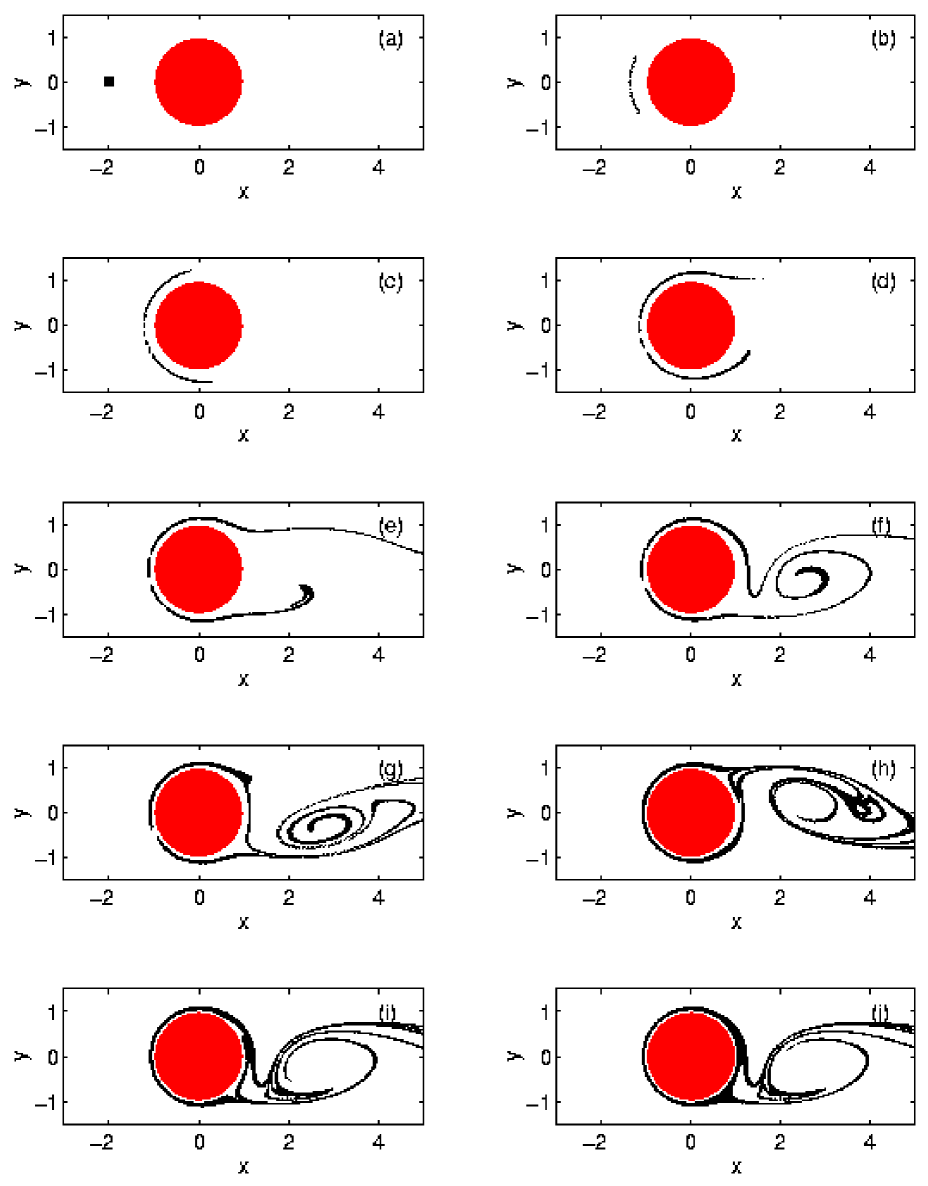
FIG. 2.: Time evolution of a seed of $400$ $B$ particles (black) placed in the flow in front of the cylinder (on a square of linear size $0.2$) at time $0$. As the auto-catalytic reaction evolves having $A$ as the background particles (white), the amount of $B$ increases and traces out a complicated object in the wake of the cylinder. After some initial increase, a steady state sets in. The snapshots (a-j) are taken at times $t=0,0.2,0.4,0.6,0.8,1.0,1.2,1.6,2.0$, and $3.0$ respectively, right before a reaction takes place. The computational domain $-3<x<5$ and $-1.5<y<1.5$ covers both the incoming and mixing regions. The time lag between reactions is $\tau=0.2$, consequently $\nu=0.072$, and the lattice size is $\varepsilon_{0}=\sigma=0.01$

To support this qualitative observation, Fig. 3 shows the number of $B$ particles in the computational domain as a function of time. After four periods, a self-repeating time dependence sets in.

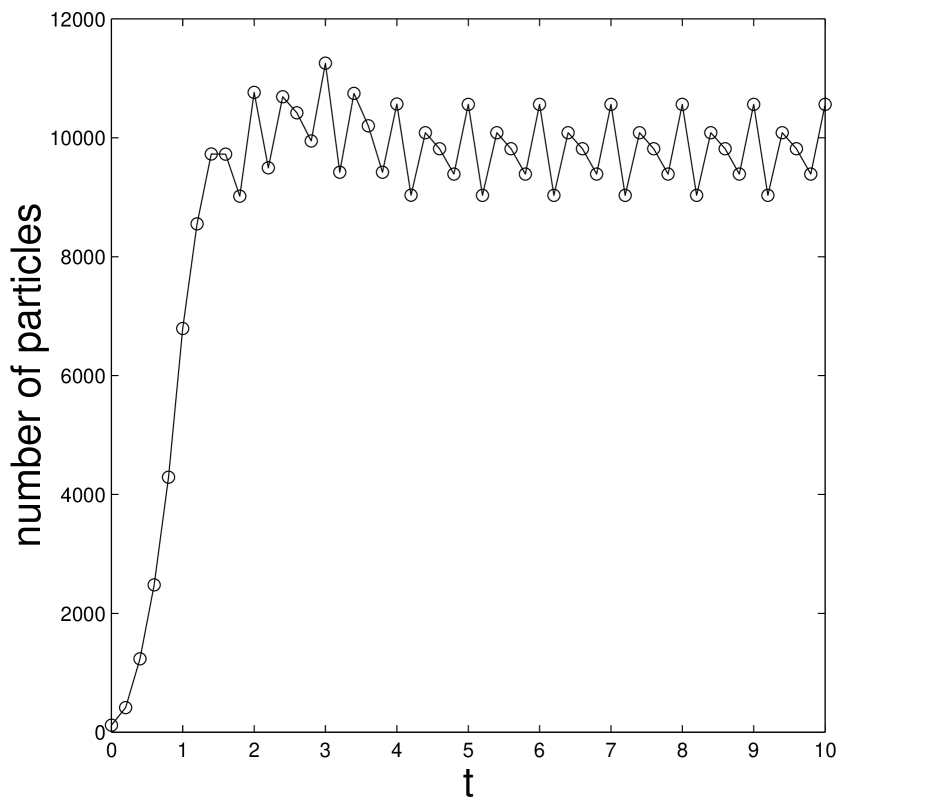
FIG. 3.: The dependence of the number ${\cal A}_{B}^{(n)}(\tau)/\varepsilon_{0}^{2}$ ($\varepsilon_{0}=\sigma$) of $B$ particles in the computational domain of Fig. 2 on time $t=n\tau$ right before the reaction events. Note the stationary time-periodic behavior reached after about four time units.

This means that the chemical reaction takes over the flow’s basic periodicity and reaches a stationary state: the number of cells being born in the reaction is the same as the number of cells escaping due to the advection dynamics.

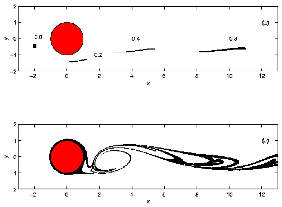
FIG. 4.: (a) Time evolution of a droplet of the same size as used in Fig. 2(a) but placed off axis for $\tau=0.2$ and lattice size $\epsilon_{0}=\sigma=0.01$. The distribution of B particles is shown at instants $t=0,0.2,0.4$ and $0.8$. No B particle is in the wake of the cylinder after a time $1.0$. (b) The same as Fig. 2(j) just in a more elongated frame. Note the downstream widening of the filaments.

In fact, owing to a special symmetry, which is not present in the case of general obstacles, the flow is reflection symmetric with respect to the $x$ axis after a time shift of one-half. Therefore, the product distribution is of period $1/2$ [34].

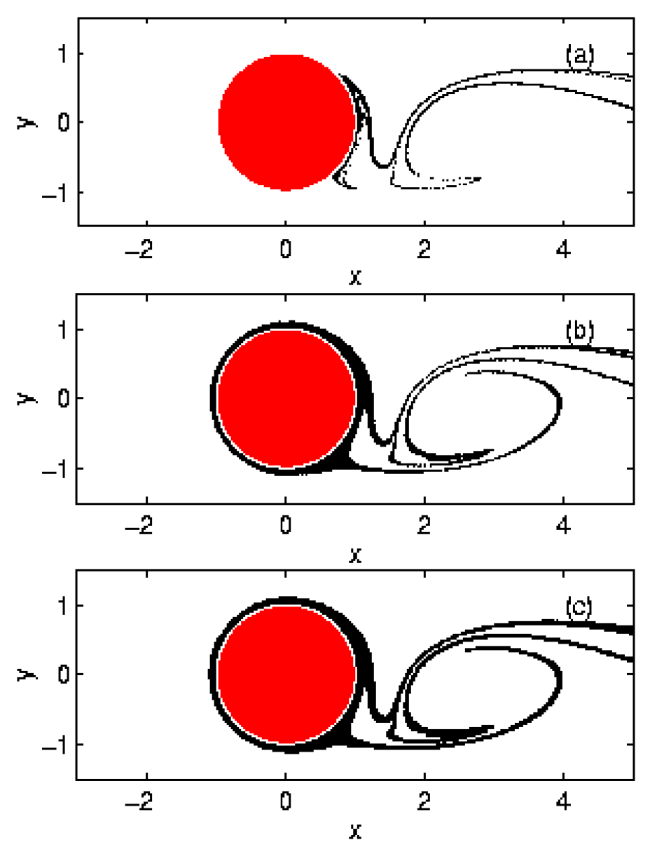
FIG. 5.: (a) The unstable manifold of the chaotic saddle in the reaction free flow generated by distributing $20.000$ passive point particles (black dots) on short segments along the local unstable direction of three basic fixed points of the Lagrangean dynamics, and iterating them forward in time over several periods. (b) and (c) shows the $B$ particle distribution at $t=10.0$ just before and just after the reaction, respectively. Note the accumulation of $B$ along the unstable manifold and note its sudden broadening from (b) to (c). The parameters are as in Fig 2.

The outcome of the dynamics depends strongly on the initial position of the seed particle. If the initial B droplet is off axis [as in Fig. 4(a)], it does not penetrate the mixing region in the wake of the cylinder, and the initial droplet is just simply stretched before the whole amount of B is washed downstream. One can observe that the size of the compact patch B increases due to the autocatalytic process as time goes on. Note that in this case no material B remains in the mixing region and the reaction dynamics dies out in any fixed observation region of finite size. This behavior is to be compared with cases where the droplet penetrates the mixing region. To sharpen the contrast, in Fig. 4(b) we display the $B$ distribution of Fig. 2(j) in a much longer region downstream. This clearly indicates that material $B$ is now present at any instant of time at any $x$-value in the wake. The gradual broadening of the stripes of product downstream is due to the autocatalytic feature of the process (and would not be present in the case of collisional reactions).

In what follows we focus on such nontrivial cases in which the droplet penetrates the mixing region. To understand the dynamics of Fig. 2, we recall that the tracer dynamics is governed by a chaotic saddle in the wake of the cylinder. Passive tracers coming close to the chaotic saddle spend a long time in the mixing region before being advected away along the unstable manifold of the chaotic saddle [cf. Fig. 5(a)]. Thus tracers having spent long time in the mixing region accumulate on the unstable manifold. A comparison of Figs. 2(i-j) and 5(a) provides numerical evidence for the accumulation of material $B$ in stripes of finite widths along this manifold.

In order to gain more insight into the reaction dynamics, Figs. 5(b) and (c) show the reagent distribution just before and just after the autocatalytic reaction takes place, respectively, in the steady state. In the first case, the $B$ distribution has a rather scanty appearance, while right after the autocatalytic reaction most of the filaments of the manifold are washed out due to a sudden widening. The two pictures correspond to two different coverages of the fractal manifold. Just before the reaction, the unstable manifold is covered with stripes of average width $\varepsilon^{*}(\tau)$, while just after the reaction with $\varepsilon^{*}(0)>\varepsilon^{*}(\tau)$. The sudden increase of the coverage width at certain times is due to our modeling of the chemical reaction as a “kicked” process. In the case of time continuous reaction obtained in the limit $\tau\rightarrow 0$ this feature is not present, but the fact that material $B$ occupies a fattened-up fractal remains unaltered. We do not want to restrict our attention to the time continuous case, because the more general setting might also be of relevance to biological phenomena, as discussed in the Introduction.

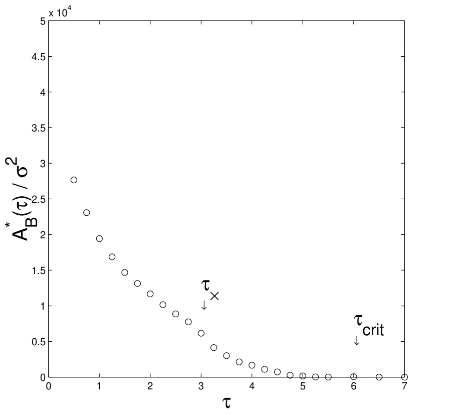
FIG. 6.: Dependence of the number ${\cal A}_{B}^{*}(\tau)/\sigma^{2}$ of $B$ particles just before reaction in the steady state on the time lag $\tau$ (all other parameters are as in Fig. 2, with the exception of the reaction range which is $\sigma=\varepsilon_{0}=0.003$, and of that a boundary layer of width $0.01$ has been cut out around the cylinder surface). Note the sudden decrease around $\tau_{\times}\approx 3$ ($\nu_{\times}\approx 1.1$), leading to a complete disappearance of $B$ from the mixing region, indicating an emptying transition, around $\tau_{crit}=6$.

One of the most interesting quantities to follow is the change of the number of $B$ particles with the time lag $\tau$ (or $\nu$) in the steady state, as shown in Fig. 6. Observe the monotonic decrease and observe that for relatively large $\tau$ values ($\tau>\tau_{crit}$) no particle remains in the wake. This indicates the existence of an “emptying transition”. For reactions taking place rather seldomly, the effect of the advection by the background flow is so strong that no $B$ particles survive the time lag $\tau$ in the wake of the cylinder, and therefore, no reaction takes place in the mixing region. Such emptying transition occurs if $\tau$ is on the order of the chaotic lifetime, and hence $\nu_{crit}\approx 1$.

B Collisional reaction: $A+B\rightarrow 2C$

Initially the flow consists of material $A$, into which we inject reagent $B$ continuously, along a line segment of length $l$ perpendicular to the background flow in front of the cylinder. As time evolves, material $C$ is produced. Figure 7 displays typical snapshots of the surroundings of the cylinder. The narrow stripes of constituent $C$ (black) separating the areas occupied by background material $A$ (white) and reagent $B$ (grey) are clearly visible. Both $B$ and $C$ stripes are now pulled along the unstable manifold of the chaotic saddle forming lobes behind the cylinder. This implies again that the reaction essentially takes place along this manifold [cf. Fig. 5(a)].

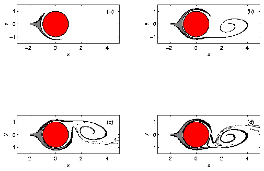
FIG. 7.: Time evolution for the collisional reaction $A+B\rightarrow 2C$. Snapshots (a-d) of the surroundings of the cylinder are taken at times $0.5,1,1.5$ and $2$, respectively, right before the reactions. The region $-3<x<5$, $-1.5<y<1.5$ is shown. Initially the flow consists of material $A$, into which we introduce reagent $B$ along the line segment $x=-2$, $-0.05<y<0.05$ ($l=0.1$). White area denotes the background material $A$, grey is reagent $B$, while black is the product $C$ separating the former constituents. The reaction range is $\sigma=0.011$, $\varepsilon_{0}=0.01$, while the time lag is $\tau=0.05$. These imply an injection rate of $14.000$ particles per unit time.

Figure 8 shows the time evolution of the number of cells occupied by $B$ and $C$. After a short transient, a saturation is reached. This means, that the number of $C$ cells born in the reaction is the same as the number of $C$ cells escaping due to the emptying dynamics.

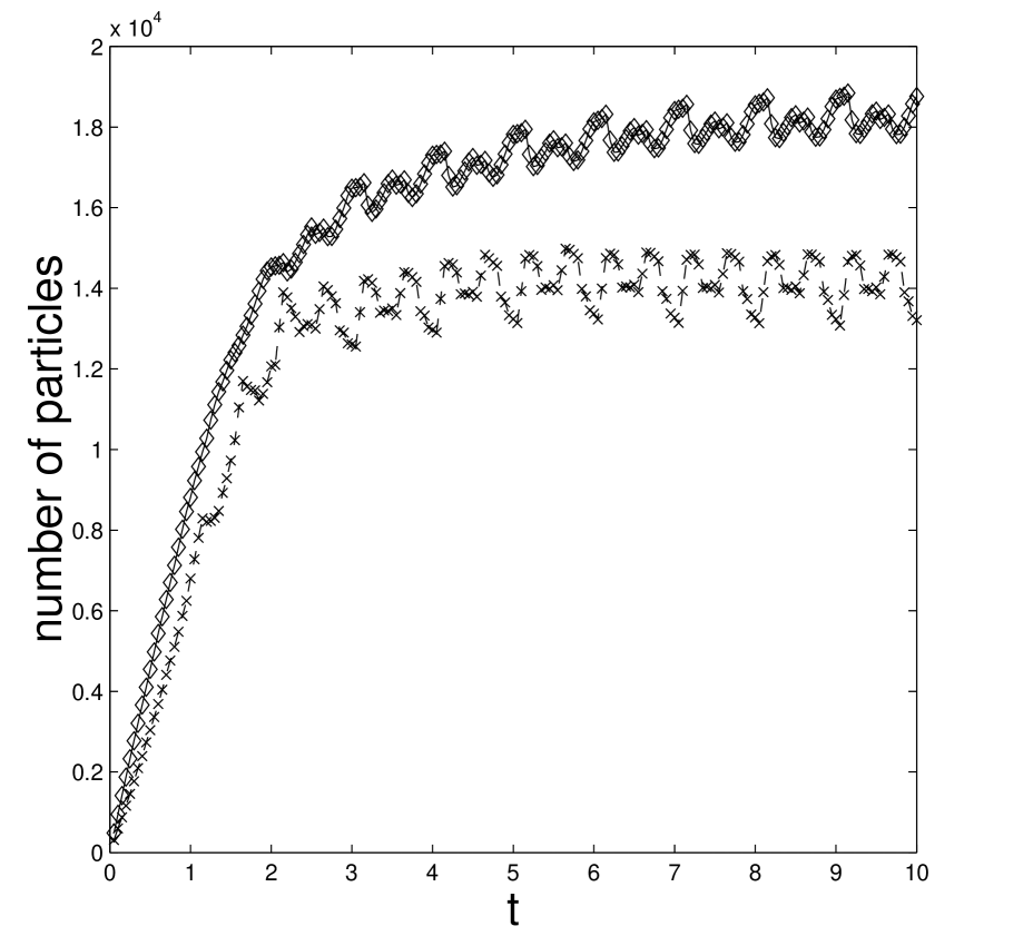
FIG. 8.: Time evolution of the number of cells occupied by $B$ (shown by diamonds) and $C$ (crosses) right before the reaction in the numerical experiment of Fig. 7. Note the asymptotic stationarity reached by both components.

As in the autocatalytic reaction, the approached stationary value of $C$ depends on the reaction range $\sigma$ and the reaction time $\nu$. The number of $B$ cells also converges to a stationary value after sufficiently long time that depends not only on $\sigma$ and $\nu$, but also on the velocity $v_{0}$ of the background flow, and on the width $l$ since the amount of inflowing $B$ per unit time is $v_{0}l$. The number of $B$ cells increases, in spite of the reaction that consumes $B$, due to the flow that brings initially more and more $B$ particles into the mixing region. A periodic pulsation can be observed after saturation has set in, just like in the autocatalytic case. By increasing the time lag $\tau$, we observe that material $B$ is not arranged along a fractal set in the wake, or does not reach the wake at all, due to the finite resolution of the grid. This already happens for not too large values of the grid size $\varepsilon_{0}$. Because we are interested in the pronounced fractal structures formed, we keep the dimensionless reaction time considerable below unity in order to ensure that activity extends into the wake along the unstable manifold.

IV Theory

A Autocatalytic reaction: $A+B\rightarrow 2B$

Basic dynamics

Let ${\cal A}_{B}(t)\equiv{\cal A}_{B}^{(n)}(s)$ denote the area occupied by reagent $B$. Here $s\in\left[0,\tau\right]$ is the time after the $n$th reaction. Thus the total physical time is $t=n\tau+s$. During the time interval of length $\tau$ only the dynamics of the chaotic flow controls the motion of the two components. In a fixed region of observation, say in a rectangle in the wake, ${\cal A}_{B}^{(n)}(s)$ decreases according to the escape rate $\kappa$ of the chaotic saddle as

$$\frac{d{\cal A}_{B}^{(n)}}{ds}=-\kappa{\cal A}_{B}^{(n)},~{}~{}~{}0\leq s<\tau,$$ (2)

provided the material is distributed along sufficiently narrow stripes around the unstable manifold at $s=0$. Solving this equation we find that the area occupied by material $B$ at the end of the interval $\tau$ is

$${\cal A}_{B}^{(n)}(\tau)={\cal A}_{B}^{(n)}(0)\;e^{-\nu}$$ (3)

with $\nu=\kappa\tau$ [35].

FIG. 9.: Schematic diagram of the components’ distribution along the unstable manifold (bold line) before and after the $n$th reaction. The borderline between the components is denoted by solid (dashed) lines before (after) the reaction. (a) Auto-catalytic reaction. (b) Collisional reaction. Here all reagents $A$ and $B$ within a distance $\sigma$ are transformed into $C$ in the course of reaction. The broadening of the half width of each $C$ stripe at reaction $n+1$ is denoted by $\zeta^{(n+1)}\geq 0$.

In order to determine the new area ${\cal A}_{B}^{(n+1)}(0)$ right after the $(n+1)$th reaction [which is expected to be larger than ${\cal A}_{B}^{(n)}(\tau)$], we recall that after sufficiently long time from the onset of the reaction [when the exponential decay law (3) holds] the area of $B$ is pulled into narrow stripes of more or less constant widths along the unstable manifold [cf. Fig. 9(a)]. In other words, the fractal unstable manifold is fattened up with material $B$ which has a nonzero area. Let $\varepsilon(t)\equiv\varepsilon^{(n)}(s)\ll 1$ denote the average width of the stripes at time $t=n\tau+s$. This means that on scales longer than or equal to $\varepsilon^{(n)}(s)$ the territory occupied by $B$ appears to be a fractal of the same dimension $D_{0}$ as the unstable manifold. Covering the full area occupied by $B$ at any time instant by squares of linear size $\varepsilon\geq\varepsilon^{(n)}(s)$, the number of boxes needed for this coverage behaves as $N(\varepsilon)={\cal H}\varepsilon^{-D_{0}}$. Here ${\cal H}$ is a constant characterizing the geometry, the so-called Hausdorff measure (or area) of the manifold. It can be obtained by determining the (unstable) manifold of the advection dynamics of the reaction-free flow. In what follows we assume ${\cal H}$ to be known.

It is worth noting that although the dimension is independent on the instant at which the snapshot is taken, the Hausdorff measure is not. Since the flow is periodic, $\cal H$ is periodic with the period of the flow: ${\cal H}(t)={\cal H}(t+1)$. (In fact, due the special reflection symmetry explained in Sec. III.A, $\cal H$ is periodic with period $1/2$.) For convenience, we choose the period of the flow to be a multiple or a divisor of the time lag: $M\tau=1$, where $M$ or $1/M$ is an integer, respectively. For time lags shorter than the flow’s period, the period contains an integer number of reactions, otherwise the time lag is an integer multiple of the period. Thus ${\cal H}^{(n)}(\tau)={\cal H}^{(n+1)}(0)$ $\equiv{\cal H}^{(n)}$ is $M$ or $1/M$ periodic as a function of $n$. Since $\varepsilon^{(n)}(s)$ is the smallest box size with which the fractality of the reagent can be felt, the area ${\cal A}_{B}^{(n)}(s)$ of $B$ can be written at any time as

$${\cal A}_{B}^{(n)}(s)={\cal H}^{(n)}(s)\;{\varepsilon^{(n)}(s)}^{2-D_{0}}.$$ (4)

To determine the dynamics of the covering width $\varepsilon^{(n)}(s)$ we observe that, at any reaction, there is a change due to the sudden increase of the product area [see Fig. 9(a)]. Since the filaments are locally smooth lines, this widening is proportional to the reaction range $\sigma$. We can thus write

$${\varepsilon^{(n+1)}(0)}={\varepsilon^{(n)}(\tau)}+\sigma d^{(n)}.$$ (5)

If the widening were exactly orthogonal to the manifold, and all the stripes occupied by $B$ were nonoverlapping, the coefficient $d^{(n)}$ would be $2$. After some time, however, initially distinct stripes start to overlap. This leads to a change in the effective free surface available for the reaction. The phenomenological factor $d^{(n)}$ introduced in Eq. (5) describes both the effect of the geometrical shapes (stripes being tilted) and the effect of overlap, on the average. It depends on the time instant $n$, and on the flow parameters. The time evolution of the shape factor $d^{(n)}$ is unknown a priori. We shall see, however, that the theory becomes consistent with the numerical observations if, after a long time, the shape factor takes over the period of the flow. Thus we assume that $d^{(n)}$ is also $M$ or $1/M$ periodic in $n$.

By taking into account Eqs. (3-4), the area ${\cal A}_{B}^{(n+1)}(\tau)$ before the $(n+1)$st reaction can be written as

$${\cal A}_{B}^{(n+1)}(\tau) = {\cal H}^{(n+1)}\left[{\varepsilon^{(n+1)}(\tau)}\right]^{2-D_{0}}$$ (6)

$$= e^{-\nu}{\cal H}^{(n)}\left[{\varepsilon^{(n+1)}(0)}\right]^{2-D_{0}}.$$ (7)

From this we find that the average widths $\varepsilon^{(n+1)}(\tau)$ just before reaction $(n+1)$ is proportional to $\varepsilon^{(n+1)}(0)$, the width right after the $n$th reaction:

$${\varepsilon^{(n+1)}(\tau)}=\varepsilon^{(n+1)}(0)\left[\frac{e^{-\nu}{\cal H}^{(n)}}{{\cal H}^{(n+1)}}\right]^{1/(2-D_{0})}.$$

Then from (5), a closed recursion relation follows for the widths just before the reactions:

$${\varepsilon^{(n+1)}(\tau)}=\left[\frac{e^{-\nu}{\cal H}^{(n)}}{{\cal H}^{(n+1)}}\right]^{1/(2-D_{0})}\;\left[{\varepsilon^{(n)}(\tau)}+\sigma d^{(n)}\right].$$ (8)

In view of Eq. (4), this implies a recursion for the $B$ area as

$${\cal A}_{B}^{(n+1)}(\tau)=e^{-\nu}\left\{\left[{\cal A}_{B}^{(n)}(\tau)\right]^{1/(2-D_{0})}+g^{(n)}\sigma\right\}^{2-D_{0}}.$$ (9)

This reaction equation is a discrete dynamics for ${\cal A}^{(n)}_{B}(\tau)$ expressing the amount of $B$ before a reaction in terms of the amount before the previous reaction. Since the quantities $d^{(n)}$ and ${\cal H}^{(n)}$ appear in a specific combination for this map, we have introduced the shorthand notation

$$g^{(n)}\equiv d^{(n)}\left.{\cal H}^{(n)}\right.^{1/(2-D_{0})}.$$ (10)

In contrast to the width dynamics (8), the area dynamics contains all geometrical contributions via $g^{(n)}$, which is called therefore the geometrical factor.

Equation (9) belongs to the same class of dynamics as recursion relations of the type $x_{n+1}=f(x_{n})$, like e.g. the famous logistic map [36]. It is one-dimensional and strongly dissipative, therefore it describes the convergence towards asymptotic motions which are represented by attractors. If ${\cal H}^{(n)}\equiv{\cal H}$ and $g^{(n)}\equiv g$ is constant, a fixed point of the system is found from ${\cal A}_{B}^{*}(\tau)={\cal A}_{B}^{(n+1)}(\tau)={\cal A}_{B}^{(n)}(\tau)$ in the form of

$${\cal A}_{B}^{*}(\tau)\equiv{\cal H}{\varepsilon^{*}}^{(2-D_{0})}=\left(\frac{\sigma g}{e^{\nu/(2-D_{0})}-1}\right)^{2-D_{0}}.$$ (11)

This is the area occupied by reagent $B$ right before a chemical reaction takes place in the stationary state. The area of $B$ right after the reaction is a factor $e^{\nu}$ larger.

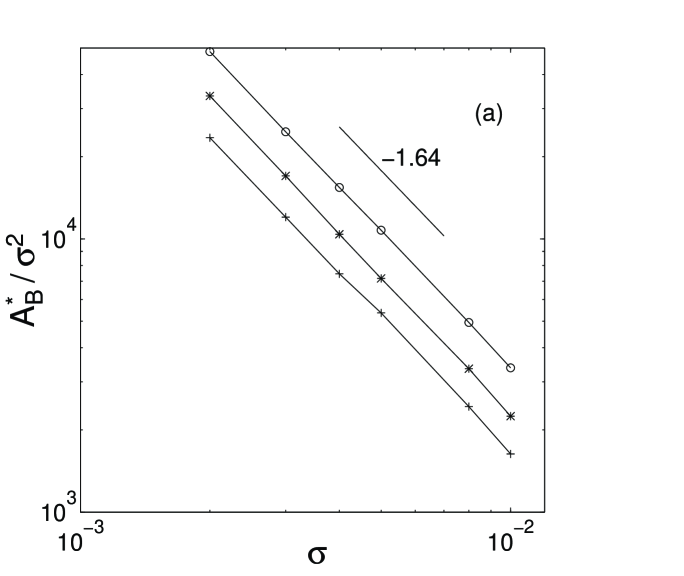
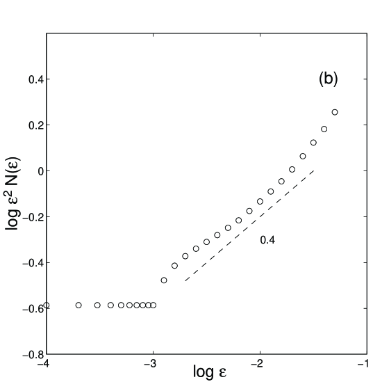
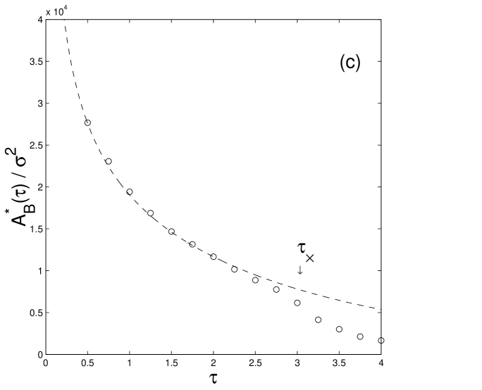
FIG. 10.: Scaling properties in the autocatalytic reaction. (a) The area ${\cal A}_{B}^{*}\equiv{\cal A}_{B}^{*}(\tau)$ occupied by $B$ in the steady state scales as ${\cal A}_{B}^{*}\sim\sigma^{2-D_{0}}$ at different values of the time lag $\tau$ (’o’ $\tau=1$, ’*’ $\tau=2$, ’+’ $\tau=3$) with $D_{0}=1.64$, in good agreement with the fractal dimension of the unstable manifold of the reaction free flow. Several runs were carried out with different values of the reaction range $\sigma$, which is set equal to the lattice constant $\sigma=\varepsilon_{0}$. (b) Number $N(\varepsilon)$ of boxes of size $\epsilon$, covering the $B$ material distribution right before the reaction, shows a fractal scaling. On the $\log_{10}{\varepsilon^{2}N(\varepsilon)}$ vs. $\log_{10}{\varepsilon}$ plot an exponent $0.4$ appears implying $D_{0}=1.6$. The crossover value is $\epsilon^{*}\approx 0.003$. Below this scale the fractal structure is completely washed out and a trivial exponent $0$ emerges. The parameters are $\sigma=0.001$, $\tau=1$. (c) The small to medium time lag range of Fig. 6, ($0<\tau<3$) fitted to (11) with $g=5.5$, $\kappa=0.36$, $D_{0}=1.61$, and $\sigma=0.003$.

In the more general case when $d^{(n)}$, ${\cal H}^{(n)}$, and thus $g^{(n)}$, are periodic with some integer $M$, a limit cycle of period $M$ is the attractor. The active process becomes thus synchronized to the underlying flow dynamics. Due to the linearity of Eq. (8), and the fact that the factor $e^{-\nu/(2-D_{0})}<1$, the limit cycle attractor of (9) is always stable (in contrast to the logistic map).

Equation (11) can be used to determine approximately the mean value of the geometrical factor $g^{(n)}$ and its oscillation amplitude about the mean in a temporally periodic steady state. For the case of Fig. 3, when the attractor is of period-5, we obtain $g=16\pm 3$. Note that for integer values of $\tau\geq 1$ (when $1/M$ is integer, too), $d^{(n)}$ and ${\cal H}^{(n)}$ are constant since the periodicity of the flow is unity. Then (11) holds again exactly.

We have carried out a series of numerical experiments for such cases to carefully check the validity of (11). Fig. 10(a) shows the scaling of $\ln{{\cal A}_{B}^{*}(\tau)}$ vs. $\ln{\sigma}$. A scaling exponent of 0.36 emerges that is close to the theoretically predicted value of $2-D_{0}\approx 0.39$.

A quantitative measure of the fractality of the $B$ pattern can be obtained by computing the “box-counting” dimension. The number of boxes of linear size $\epsilon$ that contain material $B$ is expected to scale as $\epsilon^{-D_{0}}$. Fig. 10(b) shows a fractal scaling with $1.6$ for $\epsilon>\epsilon^{*}$ and a sudden crossover at $\epsilon^{*}$ due to the fattening-up of the fractal at small scales. This $\epsilon^{*}$ is the average width of the coverage of the unstable manifold and is found to be $\epsilon^{*}=0.003\pm 0.0002$. A comparison with (11) yields that the shape factor is on the order of $d=0.6$.

Fig. 10(c) shows a fit of Eq. (11) to the measured values of ${\cal A}_{B}^{*}(\tau)$. A good quality fit has been obtained with the geometrical factor $g=5.5$ up to moderate values of the time lag $\tau$.

Observe from formula (11) that, in the limit as $\tau\to\infty$, the area of material $B$ vanishes, ${\cal A}_{B}^{*}(\tau)\to 0$. This does not necessarily mean that there is no material $B$ left in the mixing region. In fact, there is always some material $B$ left in this region, in the form of a fractal set of zero area. The $\tau\to\infty$ limit corresponds to the case where the $B$ set literally coincides with the unstable manifold of the chaotic set. Since during a reaction the $B$ set fattens up with average width proportional to $\sigma$, the fattened-up $B$ set should not have vanishing area as $\tau\to\infty$. In fact, assuming that $g^{(n)}$ is constant, and using Eqs. (3) and (11), the limit $\tau\to\infty$ gives:

$$\lim_{\tau\to\infty}{\cal A}_{B}^{*}(0)=\lim_{\tau\to\infty}e^{\nu}{\cal A}_{B}^{*}(\tau)=(\sigma g)^{2-D_{0}}\neq 0.$$ (12)

Thus, taking the limit $\tau\to\infty$ in (11) is only consistent with the chemical framework, i.e., with a continuous distribution of particles. Of course, the numerics can deal with finite grid size only. However, when the grid size is small enough, we get a good agreement with our formulas, for not too large time lags, as shown in Fig. 10(c).

Emptying transition

When deriving the theory, we do not make use of the finiteness of the grid, which can also be interpreted as the finiteness of the particle size. It is this finite size effect which leads to the emptying transition for large time lags. If during the advection dynamics of duration $\tau$ the number of escaping particles exceeds the number of new $B$ particles created at the next reaction, then the balance favors the total extinction of material $B$ from the wake. This happens at a critical value for the dimensionless reaction-time, $\nu_{crit}$ .

We derive an expression for $\nu_{crit}$ via defining the productivity of the reaction. The productivity of the chemical reaction in the steady state can be characterized by the ratio of newly-born to parent particles $B$ as

$$S=[{\cal A}_{B}^{*}(0)-{\cal A}_{B}^{*}(\tau)]/{\cal A}_{B}^{*}(\tau)=e^{\nu}-1.$$ (13)

The productivity $S$, however, cannot be arbitrarily large. An absolute maximum $S_{max}$ exists, since the number of cells inside the reaction range $\sigma$ is limited. This implies that

$$e^{\nu}-1\leq S_{max}.$$ (14)

For $\nu$ smaller than

$$\nu_{crit}=\ln{(1+S_{max})}$$ (15)

the productivity of the chemical reaction grows exponentially with increasing reaction time $\tau$ or $\nu$. For $\nu>\nu_{crit}$, however, $S$ does not grow further. Using Eq. (13) and the fact that $S\leq S_{max}$, we have

$${\cal A}_{B}^{*}(0)\leq(1+S_{max})\;{\cal A}_{B}^{*}(\tau).$$ (16)

Inserting expression (3), this leads to

$${\cal A}_{B}^{*}(0)\leq(1+S_{max})\;{\cal A}_{B}^{*}(0)\;e^{-\nu}.$$ (17)

For $\nu>\nu_{crit}$ the quantity $(1+S_{max})e^{-\nu}$ is less than $1$, therefore (17) can only hold for ${\cal A}_{B}^{*}(0)=0$. Thus, for $\nu>\nu_{crit}$, the area of reagent $B$ quickly drops to zero in time, and remains only the background material $A$ in the system in the steady state. In our case $S_{max}=8$, thus the critical reaction time lag becomes $\tau_{crit}=2\ln{3}/\kappa=6.10$. Indeed, this is confirmed by the measurements exhibited in Fig. 6.

The definition of the productivity leads us to another important time value, the crossover time lag, $\nu_{\times}$. It represents the threshold time lag of productivity for which the effects of finite particle size (and grid) come into play. Below this value, the filaments are ‘tightly’ covered by the $B$ cells, so on average one particle is responsible for at most two newborns, $S=2$. At $\nu_{\times}$, the coverage of the filaments is just about to break up, thus:

$$\nu_{\times}=\ln{(1+S)}=\ln{3}\;,$$ (18)

which leads to $\tau_{\times}=\ln{3}/\kappa=\tau_{crit}/2=3.05$. For values of $\tau$ larger than $\tau_{\times}$, the theory described in the previous paragraph breaks down since it does not make use of the finite particle size. Indeed, a deviation from (11) shows up in Fig. 6 by $\tau=3$.

The continuous time limit

Before taking the continuous time limit $\tau\rightarrow 0$, it is worth rewriting the reaction equation (9) in a different form. If the coverage of the manifold by $B$ is relatively wide, i.e., $\varepsilon^{(n)}(\tau)\gg g^{(n)}\sigma$, we can expand the right hand side of (8) to first order to obtain

$${\cal A}_{B}^{(n+1)}(\tau) = {\cal A}_{B}^{(n)}(\tau)\;e^{-\nu}$$ (19)

$$+ \sigma g^{(n)}\;(2-D_{0})\;e^{-\nu}\left[{\cal A}_{B}^{(n)}(\tau)\right]^{-\beta},$$ (20)

where

$$\beta=\frac{D_{0}-1}{2-D_{0}}$$ (21)

is a nonnegative number (it takes on zero only in nonchaotic flows). This equation is equivalent to saying that the reaction gain is proportional to the perimeter $\cal L$ of the $B$ area times the reaction range $\sigma$ [7], and that this gain can be expressed to be proportional to a power $-\beta$ of the area. [With the identification $c\equiv g^{(n)}(2-D_{0})$, Eq. (20) coincides with Eq. (3) of Ref.[7].] Because exponent $\beta$ is negative, the equation contains a singular expression of the $B$ area. The fixed point (11) for $\varepsilon^{*}$ is, in general, of the order of $g\sigma$, and the condition leading to this form is typically not valid after a long time. Therefore, Eq. (20) can only hold for a transient period before coming close to the attractor. If, however, the time lag is small enough and decreases, $\nu\ll 1$, the region of validity of (20) is increasingly longer. It is thus not surprising that in the continuous time limit, the differential equation obtained for the $B$ area is the analog of the singular map (20):

$$\dot{{\cal A}}_{B}=-\kappa{\cal A}_{B}+g(t)\;(2-D_{0})v_{r}\left({\cal A}_{B}\right)^{-\beta}.$$ (22)

Here ${\cal A}_{B}(t)$ denotes ${\cal A}_{B}^{(t/\tau)}(0)$ or ${\cal A}_{B}^{(t/\tau)}(\tau)$ for $\tau\rightarrow 0$, and

$$v_{r}=\lim_{\tau\rightarrow 0}\frac{\sigma}{\tau}$$ (23)

represents the velocity of the reaction front.

A comparison with the case of a uniform flow [Eq. (1)] shows that Eq. (22) represents a novel form of reaction equation containing a negative power of the material content due to the fractality of the unstable manifold. Its special case obtained for $D_{0}=1$ describes a surface reaction in the presence of a single isolated hyperbolic orbit in the wake

$$\dot{{\cal A}}_{B}=-\kappa{\cal A}_{B}+g(t)\;v_{r}.$$ (24)

Note that this is already structurally similar to the traditional equation (1). But even for a single periodic orbit the decay is slower than without its existence because the time scale set by the escape rate (which is now just the Lyapunov exponent of the orbit) is typically much longer than the characteristic time of the flow.

Altogether, Eq. (22) deviates in both terms from the traditional reaction dynamics (1). The decay is slower while productivity is much faster than in an unstructured flow. Both effects are due to the presence of a chaotic saddle which produces an escape rate $\kappa$ smaller than $v_{0}$ and a dimension $D_{0}$ bigger than one.

Our findings concerning the new form of the reaction equation are similar in spirit to those of Muzzio and Ottino [2]. They considered the effect of filamentation on chemical reactions in closed containers without finding an explicit form for the reaction equations. The difference with us is due to the fact that we are studying now open flows with fractal patterns of $D_{0}<2$, and our exponent $\beta$ is therefore unique.

The area occupied by $B$ in a stationary state [$g(t)=g$] follows from $\dot{{\cal A}}_{B}=0$ as

$${\cal A}_{B}^{*}\equiv{\cal H}{\varepsilon^{*}}^{2-D_{0}}=\left(\frac{g\;(2-D_{0})\;v_{r}}{\kappa}\right)^{2-D_{0}},$$ (25)

in accordance with the $\tau\rightarrow 0$ limit of Eq. (11). Equation (25) has an important consequence for the velocity of a reaction with visible fractal properties. The latter can only be seen if $\varepsilon^{*}$ is much less than unity (the cylinder radius) which implies, for $g$ factors of the order of one, that $v_{r}\ll\kappa<v_{0}$. Fractal product distributions can only be expected for reactions which are slow on the lifetime of chaos. In this continuous time limit the emptying transition does not occur, since $e^{\nu}\rightarrow 1$, and therefore (14) is fulfilled.

It is worth mentioning briefly that different continuous time limits are also possible depending on the assumptions made on the model parameters. One option is to split the reaction range $\sigma$ into a ‘deterministic’ part $\bar{\sigma}$ and a fluctuating $\delta\sigma$, i.e., $\sigma=\bar{\sigma}+\delta\sigma$. The reaction front velocity is then defined via $\bar{\sigma}$, and $\delta\sigma/\tau$ goes over as a noise term $\xi$ in the continuous time limit. So the reaction equation becomes a stochastic differential equation

$$\dot{{\cal A}}_{B}=-\kappa{\cal A}_{B}+g(t)\;(2-D_{0})\;(v_{r}+\xi)\left({\cal A}_{B}\right)^{-\beta}$$ (26)

Note that the noise term $\xi$ appears in this Langevin equation in a multiplicative form. It’s effect is thus also influenced by the fractality of the underlying manifold.

B Collisional reaction: $A+B\rightarrow 2C$

Basic dynamics

The area occupied by the materials $B$ and $C$ at time $s$ after the $n$th chemical reaction is denoted by ${\cal A}_{B}^{(n)}(s)$ and ${\cal A}_{C}^{(n)}(s)$, respectively. During the time interval $\tau$ there is no reaction, thus only the chaotic advection and the injection of $B$ governs the dynamics of the area of $B$ and $C$ as

$$\frac{d{\cal A}_{B}^{(n)}}{ds} = v_{0}l-\kappa{\cal A}_{B}^{(n)},$$ (27)

$$\frac{d{\cal A}_{C}^{(n)}}{ds} = -\kappa{\cal A}_{C}^{(n)}.$$ (28)

Here $v_{0}$ denotes the velocity of the inflow far upstream from the cylinder, and $l$ is the width of the stripe along which material $B$ is being injected in the inflow region. The rest of the inflow consists of $A$ only. After solving these equations we find the areas occupied by $B$ and $C$ right before the next reaction to be:

$${\cal A}_{B}^{(n)}(\tau) = {\cal A}_{B}^{(n)}(0)e^{-\nu}+\frac{v_{0}l}{\kappa}\;(1-e^{-\nu}),$$ (29)

$${\cal A}_{C}^{(n)}(\tau) = {\cal A}_{C}^{(n)}(0)e^{-\nu}.$$ (30)

The reaction $A+B\rightarrow 2C$ takes place if the distance between $A$ and $B$ is less then $\sigma$. Thus, the amount ${\cal A}_{B}^{(n+1)}(0)$ of material $B$ and ${\cal A}_{C}^{(n+1)}(0)$ of $C$ right after the $(n+1)$th reaction becomes smaller than ${\cal A}_{B}^{(n)}(\tau)$ and larger than ${\cal A}_{C}^{(n)}(\tau)$, respectively.

The geometry is now somewhat more involved than in the autocatalytic case. The branches of the unstable manifold are covered with material $B$ in stripes of average widths $\varepsilon_{B}^{(n)}(s)$. Adjacent to this, there are two stripes of equal widths $\varepsilon_{C}^{(n)}(s)$ containing only material $C$ [Fig. 9(b)], while material $A$ is outside. Thus, both materials $B$ and $C$ lie along a fattened-up copy of the unstable manifold. Note, however, that the amount of fattening-up is different for these materials.

In an analogous way as for the autocatalytic reaction, we introduce again a phenomenological shape factor $d^{(n)}$. Due to the effects of overlaps and non-straight geometry of the unstable manifold, we assume that a reaction takes place at time $(n+1)\tau$ if $\varepsilon_{C}^{(n)}(\tau)$ is smaller than the range $\sigma d^{(n)}$. Here $d^{(n)}$ is again dependent on the time instant, being $M$ or $1/M$ periodic in $n$ after sufficiently long times. The broadening of the half width of each $C$ stripe (which is the same as the corresponding decrease of the $B$ stripes) in the $(n+1)$th reaction is

$$\zeta^{(n+1)}\equiv\sigma d^{(n)}-\varepsilon_{C}^{(n)}(\tau).$$ (31)

This leads to the following change of the covering stripe widths:

$$\varepsilon_{B}^{(n+1)}(0)=\varepsilon_{B}^{(n)}(\tau)-2\zeta^{(n+1)},$$ (32)

and

$$\varepsilon_{C}^{(n+1)}(0) = \varepsilon_{C}^{(n)}(\tau)+2\zeta^{(n+1)}$$ (33)

$$= 2\sigma d^{(n)}-\varepsilon_{C}^{(n)}(\tau).$$ (34)

Note that Eq. (32) is meaningful only if the difference on the right hand side is non-negative. This depends on the relation between the variables $l$ and $\sigma$. For a fixed $l$, $\sigma$ can be increased independently, and at a certain value, the increase in the width of the $C$-stripes exceeds the width of the $B$ stripes during a reaction. From now on, we shall take $\sigma$ small enough, and assume that the situation in Fig. 9(b) is valid at all times during the process.

Since the fractal scaling still holds for the actual width of $B$ or $C$, at an arbitrary time, the areas are

$${\cal A}_{B}^{(n)}(s) = {\cal H}^{(n)}(s)\;\left[\varepsilon_{B}^{(n)}(s)\right]^{2-D_{0}},$$ (35)

$${\cal A}_{C}^{(n)}(s) = 2{\cal H}^{(n)}(s)\;\left[\varepsilon_{C}^{(n)}(s)\right]^{2-D_{0}}.$$ (36)

If the first equation is also applied to the inflow region, we have to assume that the width $l$ of the injection of $B$ is on the same order as $\varepsilon_{B}^{(n)}(s)$, so that its two-dimensional character cannot yet be seen on this scale. Substituting these into (30), we find two relations connecting the widths taken at different times:

$${\cal A}_{B}^{(n+1)}(\tau) = {\cal H}^{(n+1)}\left[{\varepsilon_{B}^{(n+1)}(\tau)}\right]^{2-D_{0}}$$ (37)

$$= e^{-\nu}{\cal H}^{(n)}\left[{\varepsilon_{B}^{(n+1)}(0)}\right]^{2-D_{0}}+\frac{v_{0}l}{\kappa}(1-e^{-\nu}),$$ (38)

and

$${\cal A}_{C}^{(n+1)}(\tau) = 2{\cal H}^{(n+1)}\left[{\varepsilon_{C}^{(n+1)}(\tau)}\right]^{2-D_{0}}$$ (39)

$$= 2e^{-\nu}{\cal H}^{(n)}\left[{\varepsilon_{C}^{(n+1)}(0)}\right]^{2-D_{0}}$$ (40)

with ${\cal H}^{(n)}\equiv{\cal H}^{(n)}(\tau)={\cal H}^{(n+1)}(0)$. In view of (32) and (34) we obtain a coupled set of recursions for either the stripe widths or for ${\cal A}_{B}^{(n)}(\tau)$ and ${\cal A}_{C}^{(n)}(\tau)$. The dynamics of the covering stripe width $\varepsilon_{C}$ for material $C$ has the simpler form:

$${\varepsilon_{C}^{(n+1)}(\tau)}=\left[\frac{e^{-\nu}\;{\cal H}^{(n)}}{{\cal H}^{(n+1)}}\right]^{1/(2-D_{0})}\;\left[2\sigma d^{(n)}-\varepsilon_{C}^{(n)}(\tau)\right].$$ (41)

Consequently, the change of the half width is:

$$\zeta^{(n+2)} = -\;\left[\frac{e^{-\nu}{\cal H}^{(n)}}{{\cal H}^{(n+1)}}\right]^{1/(2-D_{0})}\;\zeta^{(n+1)}$$ (42)

$$+ \sigma\;\left\{d^{(n+1)}-d^{(n)}\;\left[\frac{e^{-\nu}{\cal H}^{(n)}}{{\cal H}^{(n+1)}}\right]^{1/(2-D_{0})}\;\right\}.$$ (43)

The recursion for the stripe width $\varepsilon_{B}$ covering reagent $B$ is then obtained from Eqs. (30), (32) and (36) as

$${\varepsilon_{B}^{(n+1)}(\tau)} = \left\{\frac{v_{0}l}{\kappa{\cal H}^{(n+1)}}\;(1-e^{-\nu})\right.$$ (44)

$$+e^{-\nu}\frac{{\cal H}^{(n)}}{{\cal H}^{(n+1)}} \left.\left[{\varepsilon_{B}^{(n)}(\tau)}-2\zeta^{(n+1)}\right]^{2-D_{0}}\right\}^{1/(2-D_{0})}.$$ (45)

Finally, we find that the recursion relations for the areas are given by the following reaction equations:

$${\cal A}^{(n+1)}_{B}(\tau) = \frac{v_{0}l}{\kappa}(1-e^{-\nu})+e^{-\nu}\left[\left({\cal A}^{(n)}_{B}(\tau)\right)^{1/(2-D_{0})}\right.$$ (46)

$$+ 2\left.\left(\frac{{\cal A}^{(n)}_{C}(\tau)}{2}\right)^{1/(2-D_{0})}-2g^{(n)}\sigma\right]^{2-D_{0}},$$ (47)

$$\frac{{\cal A}^{(n+1)}_{C}(\tau)}{2} = e^{-\nu}\left[2g^{(n)}\sigma-\left(\frac{{\cal A}^{(n)}_{C}(\tau)}{2}\right)^{1/(2-D_{0})}\right]^{2-D_{0}}.$$ (48)

Here $g^{(n)}$ denotes the same geometrical factor (10) as defined for the autocatalytic process. This form implies that the area dynamics for both $B$ and $C$ only depends parametrically on $g^{(n)}$, while the $\varepsilon_{B}$ and $\varepsilon_{C}$ stripe dynamics contain $d^{(n)}$ and ${\cal H}^{(n)}$ as independent parameters.

Note that the $C$-reaction (and $\varepsilon_{C}$) is decoupled from $B$ (and $\varepsilon_{B}$), and component $B$ simply follows the $C$-dynamics: the second of Eqs. (48) is independent of the $B$ component, which may seem surprising at first sight. It was derived with the assumption that $\sigma$ is small enough, and that the average width of material $B$ is large enough to furnish enough reagent for each reaction event: the $B$ stripe is not totally consumed during an instantaneous reaction. Thus the dynamics of the reaction product $C$ depends only on the actual width of the $C$ stripes which separate $A$ from $B$. Between two consecutive reactions, the average $C$ width decreases, making possible a widening at the next reaction, and so on. Thus, the presence of $B$ is necessary for producing $C$, but if the $B$-area is wide enough, the $C$-reaction becomes independent of $B$.

In the case when the Hausdorff measure ${\cal H}$ and the shape factor $d$ (and geometrical factor $g$) are $n$-independent, we find a stationary state. The average width of the $C$ stripes can be given explicitly:

$$\varepsilon_{C}^{*}(\tau)=\varepsilon_{C}^{*}(0)\;e^{-\nu/(2-D_{0})}=\frac{2\sigma d}{e^{\nu/(2-D_{0})}+1}.$$ (49)

Consequently, from Eq. (43)

$$\zeta^{*}=\sigma\;d\;\tanh\frac{\nu}{2(2-D_{0})}$$ (50)

follows. For the average width of the $B$ stripes an implicit equation is obtained

$${\varepsilon_{B}^{*}(\tau)}^{2-D_{0}}=\frac{v_{0}l}{\kappa{\cal H}}\;(1-e^{-\nu}) + e^{-\nu}\left[{\varepsilon_{B}^{*}(\tau)}-2\zeta^{*}\right]^{2-D_{0}}.$$ (51)

Since in this equation all terms are expected to be of the same order of magnitude, we find that

$$\varepsilon_{B}^{*}\approx\left(\frac{v_{0}l}{\kappa{\cal H}}\right)^{1/(2-D_{0})}$$ (52)

holds. It means that the coverage width of the inflow of reagent $B$ is of the order of the average coverage width in the mixing range, thus our earlier assumption on the validity of Eq. (36) is fulfilled. The fixed point of recursion (41) and (43) is an attractor for any parameter since $e^{-\nu/(2-D_{0})}<1$.

The fixed point expressions for the areas occupied by $B$ and $C$ are obtained as ${\cal A}_{B}^{*}(s)={\cal H}\varepsilon_{B}^{*}(s)^{2-D_{0}}$ and ${\cal A}_{C}^{*}(s)=2{\cal H}\varepsilon_{C}^{*}(s)^{2-D_{0}}$, respectively. Thus,

$${\cal A}_{C}^{*}(\tau)\equiv 2{\cal H}{\varepsilon_{C}^{*}}^{(2-D_{0})}=2\left(\frac{2\sigma g}{e^{\nu/(2-D_{0})}+1}\right)^{2-D_{0}},$$ (53)

and

$$\left[{\cal A}_{B}^{*}(\tau)e^{\nu}+\frac{v_{0}l}{\kappa}(1-e^{\nu})\right]^{1/(2-D_{0})}={{\cal A}_{B}^{*}(\tau)}^{1/(2-D_{0})}$$ (54)

$$- 2g\sigma+2\left(\frac{{\cal A}_{C}^{*}(\tau)}{2}\right)^{1/(2-D_{0})}.$$ (55)

Note that although (53) is in some sense the analogue of (11), the particular $\nu$-dependence is different: we have now a Fermi-Dirac distribution, while (11) was of Bose-Einstein type. This difference is due to the fact that the increase of $\varepsilon_{C}$ in a reaction step is not a constant, rather it is proportional to $\zeta$ which also depends on $\varepsilon_{C}$ itself [cf. (34)]. From these two relations a $g$-independent form follows

$$\left[{\cal A}_{B}^{*}(\tau)e^{\nu}+\frac{v_{0}l}{\kappa}(1-e^{\nu})\right]^{1/(2-D_{0})}={{\cal A}_{B}^{*}(\tau)}^{1/(2-D_{0})}$$ (56)

$$+ \left(1-e^{\nu/(2-D_{0})}\right)\;\left(\frac{{\cal A}_{C}^{*}(\tau)}{2}\right)^{1/(2-D_{0})},$$ (57)

which does not contain any free parameters.

When the periodicity of ${\cal H}$, $d$ and $g$ is pronounced, recursions (48) typically possess a limit cycle attractor corresponding again to a full synchronization to the flow dynamics.

The consistency of expressions (53), (55) and (57) with the numerics is verified in different ways (we fixed $v_{0}=14$ and $l=0.1$). The comparison of the results shown for a period 20 limit cycle steady state in Fig. 8 with the expression (53) yields $g=42\pm 4$ for the geometrical factor. This value is also consistent with (55) and the measured $B$ area. In simulations using different grid sizes $\varepsilon_{0}$, we find similar geometrical factor values that are slightly increasing with $\varepsilon_{0}$. We also evaluate the ratio of the left and right hand sides of the fit-free relation (57) at different grid sizes $\varepsilon_{0}=0.007$, $0.01$ and $0.013$ and time lags $\tau=1/80,1/40,1/20$ and $1/10$. The ratio is in all cases between 0.9 and 1.0 with an average $0.96\pm 0.05$, $0.95\pm 0.04$ and $0.94\pm 0.03$ for the $\varepsilon_{0}$ values investigated, respectively. In view of the fact that $g^{(n)}$ is not a constant, since the time lag is definitely below unity, the agreement, within an accuracy of 10 percent is satisfactory because this is exactly the amplitude of fluctuations in $g$.

The continuous time limit

Before taking the time continuous limit $\tau\rightarrow 0$, it is worth again rewriting the reaction equation (48) in a different form. If the coverage of the manifold by $B$ and $C$ is large with respect to the amount of broadening, i.e., if $\varepsilon_{B}^{(n)}(\tau),\varepsilon_{C}^{(n)}(\tau)\gg\zeta^{(n+1)}$, we can expand the right hand sides of (48) to first order in $\zeta$ using (41) and (45) to obtain

$${\cal A}^{(n+1)}_{B}(\tau)={\cal A}^{(n)}_{B}(\tau)e^{-\nu}+\frac{v_{0}l}{\kappa}\;(1-e^{-\nu})$$ (58)

$$- 2(2-D_{0})e^{-\nu}\;\frac{\zeta^{(n+1)}}{d^{(n)}}g^{(n)}\left[{\cal A}^{(n)}_{B}(\tau)\right]^{-\beta},$$ (60)

$$\frac{{\cal A}^{(n+1)}_{C}(\tau)}{2}=\frac{{\cal A}_{C}^{(n)}(\tau)}{2}e^{-\nu}$$

$$+ 2(2-D_{0})e^{-\nu}\;\frac{\zeta^{(n+1)}}{d^{(n)}}g^{(n)}\left[\frac{{\cal A}^{(n)}_{C}(\tau)}{2}\right]^{-\beta}.$$ (61)

Here $\beta$ is the same exponent (21) as in the autocatalytic reaction. The fixed point (49) for $\varepsilon_{C}^{*}$ is, in general, on the order of $\zeta^{*}$ and the condition leading to this form is typically not valid after a long time. Therefore, Eq. (61) can only hold for a transient period before coming close to the attractor. If, however, the time lag is small enough and decreases, $\nu\ll 1$, the region of validity of (61) is increasingly longer.

Next we take the continuous time limit. Let $f(t)$ denote the $\tau\rightarrow 0$ limit of any function which takes the form $f^{(n)}(s)$ at time $t=n\tau+s$ in the discrete time representation, with $t$ kept fixed. Let us first consider the recursion (43) of $\zeta$ and divide it by the shape factor $d$. The basic observation is that due to the minus sign in the first term on the right hand side, the recursion in the limit $\tau\rightarrow 0$ does not go over into a differential equation for $\zeta/d$. Rather it shows that this ratio goes to zero linearly with the time lag. Therefore it is natural to define a reaction front velocity as

$$v_{r}(t)=\lim_{\tau\rightarrow 0}\frac{\zeta^{(n+1)}}{\tau d^{(n)}}.$$ (62)

It should be emphasized that this property means that the broadening of the $C$ stripes should tend to zero in the continuous time limit. Therefore, at any time $\varepsilon_{C}(t)=\sigma d(t)$ holds. Thus, in contrast to the autocatalytic reaction, the reaction range needs not to go to zero now, since another quantity, the actual broadening has to. In fact, $\sigma$ is finite, and is a measure of the front velocity. A substitution of this form into (43) yields the explicit expression

$$v_{r}=\frac{\sigma}{2}\left[\frac{\kappa}{(2-D_{0})}+\frac{d}{dt}\ln{g(t)}\right].$$ (63)

Since $g$ is periodic with the flow’s periodicity, the front velocity is also periodic.

From recursion (61) we obtain for the differential equations of the $B$ and $C$ areas in the limit $\tau\rightarrow 0$

$$\dot{{\cal A}}_{B} = -\kappa{\cal A}_{B}+v_{0}l-q(t)\left({\cal A}_{B}\right)^{-\beta},$$ (64)

$$\dot{{\cal A}}_{C}/2 = -\kappa{\cal A}_{C}/2+q(t)\left({\cal A}_{C}/2\right)^{-\beta},$$ (65)

where the coupling constant in both equations is the same $q(t)=$ $2(2-D_{0})$ $v_{r}(t)g(t)$. The two dynamics become entirely decoupled in this limit. Notice the singular terms on the right hand sides again.

The fixed point value of the $C$ area [for $d(t)\equiv d$, ${\cal H}(t)\equiv\cal H$, $q(t)\equiv q$] is

$${\cal A}_{C}^{*}=2(q/\kappa)^{2-D_{0}}$$ (66)

The $B$ area has also a fixed point solution, but it is implicit:

$${\cal A}_{B}^{*}={\cal H}{\varepsilon_{B}^{*}}^{2-D_{0}}=\frac{v_{0}l}{\kappa}-\frac{q}{\kappa}\left[{\cal A}_{B}^{*}\right]^{-\beta}.$$ (67)

The front velocity

$$v_{r}=\frac{\sigma\kappa}{2(2-D_{0})}=\frac{q}{2(2-D_{0})g}$$ (68)

is now a constant entirely determined by the reaction free flow’s parameters and the reaction range. This implies $\varepsilon_{C}^{*}=d\sigma$ in accordance with the $\nu\rightarrow 0$ limit of equation (49).

V Discussion

First we discuss a few aspects of the nonlinear dynamics which has not been mentioned in the text.

The stable manifold is a fractal curve leading particles to the chaotic saddle. Points lying close to it reach the saddle rapidly, and their long lifetime is due to a residence time in the neighborhood of the saddle. In other words, initial conditions close to or far away from the stable manifold lead to considerable lifetime differences only after the saddle region has been reached. Thus, although the role of stable and unstable manifolds seems to be symmetric in the problem, the residence about the stable manifold is not long enough for an enhancement in activity. Therefore, no fattening-up takes place along this manifold. Anyhow, a nontrivial reaction can only occur if the $B$ (and $C$) initial conditions intersect the stable manifold. Otherwise, cases like the one shown in Fig. 4(a) occur without a fractal product distribution.

The advection dynamics is known to have a considerable nonhyperbolic component consisting of points lying very close to the cylinder surface. The nonhyperbolic part is characterized by a nonexponential decay ($\kappa=0$) and space-filling fractality ($D_{0}=2$) [29]. Previous studies [20, 21] have shown, however, that in the von Kármán flow model the resolution allowed in computer simulations is still too crude to observe the nonhyperbolic effects away from (but close to) the cylinder surface. The relative strength of the hyperbolic component ensures that on the time and length scales used we are able to work with a nontrivial fractal dimension and a finite escape rate. Apart from the nonhyperbolicity seen in the boundary layer around the obstacle, other nonhyperbolic structures are expected to be seen on very small scales only. The presence of a finite coverage with widths $\varepsilon^{*}$, however, prevents us to reach these scales. This is why the properties of the hyperbolic component play essential role in the full process. Therefore, in any fixed frame in the wake not overlapping with the boundary layer, the results of the theory presented here are expected to hold [37].

Next we summarize those features of our model which are believed to be general for active processes accompanied by weak diffusion in open flows with velocities faster than that of the reaction.

$\bullet$ Active processes take place about the unstable manifold of the passive dynamics’ invariant set. If the dynamics is chaotic, the manifold is a fractal and, consequently, the reaction leads to fractal patterns.

$\bullet$ Although the fractal itself is a set of measure zero, the chemical products are of finite amount due to the fattening up process.

$\bullet$ The fractal backbone results in an increase of the active surface, it acts as a catalyst, and generates an enhancement in activity as compared to flows with nonchaotic particle dynamics.

$\bullet$ The inclusion of weak molecular diffusion in the model can be regarded as a random walk superimposed on the deterministic advection. This would result in a further fattening-up of the fractal set, in a renormalization of $\sigma$ and thus of $\varepsilon^{*}$.

$\bullet$ As a formal consequence of the fractal backbone, the product of the reaction obeys a singular scaling law.

$\bullet$ In spite of the passive tracers’ Hamiltonian dynamics, the active processes’ equations are of dissipative character possessing attractors.

$\bullet$ Most typically, a kind of steady state sets in after sufficiently long times, a state which is synchronized with the flow’s temporal behavior.

$\bullet$ Fractality is independent on whether the traditional reaction equations are linear or nonlinear since it is a consequence of the advection dynamics’ strong nonlinearity.

$\bullet$ The essential parameters for the chemical reaction in the flow depend on the parameters of the reactionless dynamics: the escape rate $\kappa$ and fractal dimension $D_{0}$. These in turn depend on parameters (like the Reynolds number) of the underlying hydrodynamics.

$\bullet$ The derivation of the reaction equations is similar to the derivation of macroscopic transport equations from microscopic molecular dynamics. It seems that the presence of ever refining fractal structures (which cannot be observed directly with finite resolution) generate new terms in the reaction equation leading to observable macroscopic effects based on the fractal microstructures. They appear not only in the averages but also in moments if a stochastic description is used.

All these features are expected to be present in realistic chemically or biologically active environmental flows observed on finite time scales.

REFERENCES

- [1] G. Metcalfe and J. M. Ottino, Phys. Rev. Lett. 72, 2875 (1994); Chaos Solitons Fractals 6, 425 (1995).
- [2] F. J. Muzzio and J. M. Ottino, Phys. Rev. A 40, 7182 (1989); Phys. Rev. A 42, 5873 (1990)
- [3] I. R. Epstein, Nature 374, 321 (1995)
- [4] S. Edouard, B. Legras, B. Lefevre, and R. Eymard, Nature 384, 444 (1996); S. Edouard, B. Legras, and V. Zeitlin, J. Geophys. Res. 101 (D11), 16771 (1996);
- [5] M. P. Chipperfield et al., J. Gephys. Res. 102, 1467 (1997)
- [6] M. G. Balluch and P. H. Haynes, J. Gephys. Res. 102, 23 487 (1997)
- [7] Z. Toroczkai, G. Károlyi, Á. Péntek, T. Tél, and C. Grebogi, Phys. Rev. Lett. 80, 500 (1998).
- [8] D. G. H. Tan, P. H. Haynes, A. R. MAcKenzie, and J. A. Pyle, Effects of fluid-dynamical stirring and mixing on the deactivation of stratospheric chlorine, J. Geophys. Res., in press
- [9] A. Mariotti, C. R. Mechoso, and B. Legras, Ozone filaments from the southern polar night vortex, J. Gephys. Res., submitted
- [10] H. Lustfeld and Z. Neufeld, Chemical dynamics versus transport dynamics in a simple model, submitted preprint.
- [11] J. M. Ottino, The kinematics of mixing: stretching, chaos and transport, (Cambridge University Press, Cambridge, 1989); J. M. Ottino, Ann. Rev. Fluid Mech. 22, 207 (1990); S. C. Jana, G. Metcalfe and J. M. Ottino, J. Fluid Mech. 269, 199 (1994).
- [12] A. Crisanti et al., Riv. Nuov. Cim. 14, 1 (1991).
- [13] Chaos, Solitons, Fractals 4, No.6 (1994), special issue on Chaotic Advection, ed. by H. Aref
- [14] D. K. Kondepudi, R. J. Kaufman, and N. Singh, Science 250, 975 (1990); S. Cortassa, et al., Biochem. J 269, 115 (1990).
- [15] P. M. Holligan et a., Global Biogeochem. Cycles 7(4), 879 (1993).
- [16] W. H. Thomas, and C. H. Gibson, J. Appl. Phycology 2, 71-77 (1990); Deep Sea Res. 37 (10), 1583-93 (1990); C. H. Gibson, and W. H. Thomas, J. Geophys. Res. 100 (C12), 24841-46 (1995).
- [17] V. Rom-Kedar, A. Leonard and S. Wiggins, J. Fluid. Mech. 214, 347 (1990).
- [18] K. Shariff, T. H. Pulliam and J. M. Ottino, Lect. Appl. Math. 28, 613 (1991).
- [19] C. Jung and E. Ziemniak, J. Phys. A 25, 3929 (1992); C. Jung and E. Ziemniak, in: Fractals in the Natural and Applied Sciences, Ed.: M. M. Novak, (North Holland, Amsterdam, 1994); E. Ziemniak and C. Jung, Phys. Lett. A202, 263 (1995)
- [20] C. Jung, T. Tél and E. Ziemniak, Chaos 3, 555 (1993).
- [21] E. Ziemniak, C. Jung and T. Tél, Physica D 76, 123 (1994).
- [22] D. Beigie, A. Leonard, and S. Wiggins, Chaos Sol. Fract. 4, 749 (1994).
- [23] Á. Péntek, T. Tél, and Z. Toroczkai, J. Phys. A 28, 2191 (1995); Fractals 3, 33 (1995).
- [24] Á. Péntek, Z. Toroczkai, T. Tél, C. Grebogi, and J. A. Yorke, Phys. Rev. E51, 4076 (1995).
- [25] J. Kennedy and J. A. Yorke, The topology of stirred fluids, in print (1997).
- [26] M. A. Sanjuan, J. Kennedy, C. Grebogi, and J. A. Yorke, Chaos 7, 125 (1997).
- [27] Z. Toroczkai, G. Károlyi, Á. Péntek, T. Tél, C. Grebogi and Y. A. Yorke, Physica A 239, 235 (1997).
- [28] J. C. Sommerer, H.-C. Ku, and H. E. Gilreath, Phys. Rev. Lett. 77, 5055 (1996)
- [29] T. Tél, in: Directions in Chaos, vol. 3, Ed.: Hao Bai-Lin, Transient Chaos: a Type of Metastable State, in: STATPHYS’19, ed.: Bai-Lin Hao (World Scientific, Singapore, 1996) pp: 346-62 (World Scientific, Singapore, 1990) pp. 149-221
- [30] L. D. Landau, and E. M. Lifschitz, Fluid Mechanics, 2nd ed. (Pergamon Press, Oxford, 1987).
- [31] D. McKenna, private communication
- [32] A. Mariotti, private communication
- [33] For the case II.A (II.B) a cell can have more than one preimages (images) due to the lattice dynamics. This means that the number of the product particles is slightly decreasing (increasing) in time compared to one in the continuum description of the flow. The use of the different lattice dynamics is motivated by the observation that the loss of generated by the method II.A is compensated by the strong autocatalytic spreading, while the same choice would have led to an underestimation of product in the collisional reaction.
- [34] For general values of , when there is no reaction exactly at time or , the period of the fluctuations in the number of particles is the smallest common multiple of 1/2 and .
- [35] Due to the periodic motion of the unstable manifolds’ lobes, there might be a small oscillatory component present in the decay dynamics. The decay rate of (2) should be replaced by with as a periodic function of small amplitude. In this case can be expressed via an integral of the time-dependent decay rate.
- [36] K. T. Alligood, T. D. Sauer, and J. A. Yorke, An Introduction to Dynamical Systems (Springer, Berlin, 1997)
- [37] By not cutting out the boundary layer, we find that relation (11) is still valid but with an effective escape rate smaller than . This value, however, is dependent on details, like the time of observation or the position of the frame. Interestingly, it is only the escape rate, whose value is influenced considerably by the presence of the boundary layer. Cutting out a layer of width does not modify the fractal dimension extracted from Figs. 10(a),(b).