[

Quasiclassical Surface of Section Perturbation Theory

Abstract

Perturbation theory, the quasiclassical approximation and the quantum surface of section method are combined for the first time. This solves the long standing problem of quantizing the resonances and chaotic regions generically appearing in classical perturbation theory. The result is achieved by expanding the ‘phase’ of the wavefunction in powers of the square root of the small parameter. It gives explicit WKB-like wavefunctions even for systems which classically show hard chaos. We also find analytic solutions to some questions raised recently.

]

Perturbation expansions in a small parameter $\epsilon$ are important in both classical and quantum physics. Not only are valuable approximations produced, but the breakdown of the expansion can signal new physics.

Poincaré found that classical perturbation theory [PT] on an integrable system fails in two [or more] dimensions for any $\epsilon,$ due to ‘small denominators’. The Kolmogorov-Arnol’d-Moser [KAM][2] theory greatly illuminated the subject and showed that the breakdown of PT signals chaos. Phase space trajectories of an integrable system lie on invariant tori. Under perturbation, periodic orbits, on ‘rational’ tori, are destroyed except for one or more stable and unstable orbits. The rational tori are labelled by $p,q$, where $p$ is the winding number and $q$ is the number of returns to the SS per period. New invariant tori are formed around the stable orbits while chaos develops near the unstable orbit. The original tori near the rational one are also destroyed, to a width in action $\sqrt{\epsilon}S_{pq}.$ The characteristic action $S_{pq}$ generically drops off rapidly with $q.$ This is usually pictured, as in Fig.1, on a surface of section [SS], a slice through the tori, where the structure of alternating stable and unstable orbits is called an ‘island chain’ or ‘resonances’.

Quantization of such a system has been of great interest. A rule of thumb is that only phase space structures of area Planck’s constant $h$ or greater are reflected in the quantum result. Thus, if $\sqrt{\epsilon}S_{pq}<<\hbar$ ordinary quantum perturbation theory works well. Above the ‘Shuryak border’ [SB][3], $\sqrt{\epsilon}S_{pq}\geq\hbar$, ordinary perturbation theory breaks down as a number $\sqrt{\epsilon}S_{pq}/\hbar$ unperturbed quantum states are strongly mixed by the perturbation. Thus quantum perturbation theory for small $h$ depends critically on the relation between $\hbar$, $\sqrt{\epsilon},$ and the torus $p,q.$

Small $h$ is not a perturbation: rather the quasiclassical approximation [QCA] is used. Combined QCA and PT has been studied over the years: the perturbed trace formula most recently[4]. The SB does not appear in [4], because effectively only short times are considered, where classical perturbation theory does work.

We here combine for the first time, PT, the QCA, and the powerful QCA-SS method of Bogomolny[5, 6]. We achieve quite complete and explicit results. Namely, we are able to find all the energy levels and wavefunctions in a WKB approximation for small $\epsilon,$ provided $h$ is not too small in a sense to be specified. Interestingly enough, we are led to express the wavefunctions in terms of a phase $G$ which is generically expanded as a series in $\sqrt{\epsilon}$ rather than $\epsilon$. This series is generated in a novel recursive way: A partial $n-1$’th order solution is obtained which allows a partial $n$’th order solution which in turn gives the complete $n-1$’th order and a partial $n+1$’th order, and so on. We also give some numerical checks.

A number of problems susceptible to this new technique have appeared recently[7, 8, 9], and we have also learned of several ongoing efforts[10]. These problems are related to a weakly deformed circular billiard. The Helmholtz equation $\left(\nabla^{2}+k^{2}\right)\Psi=0$ is to be solved for eigenfunctions $\Psi=\Psi_{a}$ and eigenvalues $k=k_{a}$ with, say, Dirichlet conditions $\Psi_{a}(r,\theta)=0$ on the boundary, $\partial B$. The latter is expressed in polar coordinates by $r(\theta)=R_{0}+\epsilon\Delta R(\theta).$ These and similar boundary perturbations have heretofore been treated [11] by methods valid only below the SB.

We illustrate with the stadium billiard[8] which has two semicircular endcaps of radius $R_{B}$ connected by parallel straight sides of length $2a$. Then $\epsilon=a/R_{B}$ is assumed small and $R_{0}$ is taken as $R_{0}\approx R_{B}+2a/\pi$ while $\Delta R/R_{0}\approx\left|\sin\theta\right|-2/\pi.$ This ‘stadium’ choice of $\Delta R$ has a discontinuous first derivative so KAM does not apply. Fig. 1a shows that the classical map deviates from the new invariant tori [given approximately by $l_{WKB}(\theta)$ defined below] after about $1/\sqrt{\epsilon}$ iterations. We also show results, Fig. 1b, for a ‘smoothed stadium’, a truncated Fourier series of the ‘stadium’ $\Delta R(\theta)$, where the orbit stays on a new invariant torus.

Classically the stadium is chaotic with no stable orbits. Orbits diffuse in angular momentum at long times[8]. It was thought that such hard chaos systems do not have simple, analytically expressible wavefunctions when quantized. Thus, qualitative and statistical questions, such as the existence and statistics of localization, have been considered. Our explicit analytic results were therefore quite unexpected, and we are able to interpret the results directly in terms of analytic wave functions. The results are possible because it is the short time, nearly regular behavior which determines the quantization.

In quantum language, we take units $R_{0}=1,$ $\hbar=1,$ particle mass = $1/2$, so $k$ is the dimensionless wavenumber, [equivalent to $1/\hbar$]. We take the billiard boundary $\partial B$ as SS. Then Bogomolny’s unitary operator is[5]

$$T(\theta,\theta^{\prime},k)=-\left(\frac{k}{2\pi i}\frac{\partial^{2}L(\theta,\theta^{\prime})}{\partial\theta\partial\theta^{\prime}}\right)^{\frac{1}{2}}\exp\left(ikL\left(\theta,\theta^{\prime}\right)\right)$$ (1)

where $L$ is the chord distance between two points, specified by polar angles, on $\partial B$. Expanding,

$$kL(\theta,\theta^{\prime}) = 2k\left|\sin\frac{\theta-\theta^{\prime}}{2}\right|\left(1+\epsilon\frac{\Delta R(\theta)+\Delta R(\theta^{\prime})}{2}\right)+\ldots$$ (2)

$$= k(L_{0}+\epsilon L_{2}+\ldots.)$$ (3)

The energy levels [$k_{a}$] of the system are given in QCA[5] by solution of $\det(1-T(k))=0$. Our seemingly more difficult technique studies

$$\psi(\theta)=\int d\theta^{\prime}T(\theta,\theta^{\prime},k)\psi(\theta^{\prime}),$$ (4)

solvable only for $k=k_{a}.$ [$\psi\approx\partial\Psi/\partial n$ on $\partial B$.]

We start with the Ansatz $\psi(\theta)=\exp\left(i\alpha f(\theta)\right)$ where $df/d\theta=$ $f^{\prime}$ $\sim 1$ and $k>>\alpha>>k\epsilon$. This Ansatz represents a superposition of angular momentum states $\left|l\right|\sim\alpha<<l_{\max}=k,$ and for $\alpha>1$ conveniently expresses the mix of states needed to diagonalize the Hamiltonian above the SB.

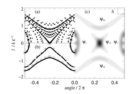
FIG. 1.: SS [angular momentum vs angle] of orbits for a) ‘stadium’ and b) ‘smoothed stadium’ $\epsilon=0.01$. Points on $l_{WKB}(\theta),\,$ for ‘continuum’,$\Diamond$, ‘separatrix’,$+,$ and ‘bound’, $*$, values of $E_{m},$ respectively. Three orbits, each iterated 1000 times, coalesce into solid lines in b), where KAM applies. Orbits started at the symbols iterated forward and backward 15 times appear as dots in a) where KAM fails. Only short time structure is regular. c) Husimi plots for exact states of Fig. 2, as well as a ‘scar’ state $\psi_{32}$. Square has area $h.$

According to the stationary phase [S$\Phi$] method, the $\theta^{\prime}$ integral is dominated by the region $\theta^{\prime}\sim\theta\pm\pi$ where $kL_{0}=2k\left|\sin\frac{1}{2}(\theta-\theta^{\prime})\right|$ is stationary.  Expand $\sin\frac{1}{2}(\theta-\theta^{\prime})\approx 1-\frac{1}{8}\delta\theta^{2}$ , $\delta\theta=\theta^{\prime}-\theta-\pi$ to find

$$S(\theta,\theta^{\prime})=kL\approx 2k-{\textstyle{1\over 4}}k\delta\theta^{2}+k\epsilon(\Delta R(\theta)+\Delta R(\theta^{\prime}))$$ (5)

[In Eq.(5) we replaced $L_{0}$ by $2$, its stationary value, when multiplied by $\epsilon.$]

Regarding $S$ as a classical generating function, we obtain the surface of section maps $(l^{\prime},\theta^{\prime})\rightarrow(l,\theta)$ found earlier[8],[9] by $l=\partial S/\partial\theta,$ $l^{\prime}=-\partial S/\partial\theta^{\prime}$. Motivated by this, Borgonovi[10] has studied the $T$ operator and classical map given by Eq.(5) with $\Delta R=\left|\sin\theta\right|$ and $\delta\theta=\theta^{\prime}-\theta$ . This system is ‘almost’ the quantum kicked rotor-classical standard map[12], which corresponds to $\Delta R=\sin\theta$. Thus, in addition to solving the distorted billiard problem, we can also solve an important class of quantized perturbed twist maps.

Returning to Eq.(4), we expand all functions of $\theta^{\prime}$ about $\theta+\pi.$ I.e. $f(\theta^{\prime})\approx f(\theta+\pi)+\delta\theta\,f^{\prime}(\theta+\pi)$ to order $\delta\theta$, [since $\alpha<<k$] and $\Delta R(\theta^{\prime})\approx\Delta R(\theta+\pi),$ since $\alpha>>k\epsilon$. Doing the integral reduces Eq.(4) to

$$\exp[i\alpha f(\theta)]$$ (6)

$$= i\exp\left[i\left(2k+(\alpha f^{\prime})^{2}/k+k\epsilon V(\theta)+\alpha f(\theta+\pi)\right)\right]$$ (7)

where $V(\theta)=\Delta R(\theta)+\Delta R(\theta+\pi).$

For Eq.(7) to hold, the exponents of order $\alpha$ must combine to give a constant $c$, i.e. $f(\theta+\pi)=f\left(\theta\right)+c.$ Now take $\alpha=k\sqrt{\epsilon}$ so a solution is possible provided $(f^{\prime})^{2}+V(\theta)$ is a constant, which we call $E_{m}$. Thus

$$f(\theta)=\pm\int_{0}^{\theta}d\theta^{\prime}\sqrt{E_{m}-V(\theta^{\prime})}$$ (8)

reminiscent of elementary WKB theory. The constant of integration is irrelevant. Notice $V(\theta)=V(\theta+\pi)\Longrightarrow f(\theta+\pi)=f\left(\theta\right)+c.$ We define $l_{WKB}(\theta)=k\sqrt{\epsilon}f^{\prime}(\theta).$

Assuming for now that $E_{m}\geq V$ , [a ‘continuum’ state], we must choose $E_{m}$ such that $kb\int_{0}^{2\pi}d\theta^{\prime}\sqrt{E_{m}-V(\theta^{\prime})}=2\pi m$ where $m$ is integer, $b=\sqrt{\epsilon}$ and so $c=\pi m/kb.$ The condition giving the energy is

$$\exp\left[i\left(2k+kb^{2}E_{m}+kbc+\pi/2\right)\right]=1=\exp(2\pi in)$$ (9)

which has solutions $k=k_{n,m}.$ For $\Delta R=0$, this reduces to $2k+m^{2}/k+\pi m=(n-\frac{1}{4})2\pi$ equivalent to Debye’s approximation to Bessel’s function, valid for $k$ large and $m/k$ small. Thus, this Ansatz produces states labelled $m,n$ with $m$ an integer angular quantum number satisfying $\left|m\right|<<k_{n,m}\approx\pi n.$ There are three symmetries, reflections about the two principal axes and time reversal, which allows real wavefunctions. Thus the even-even states are $\psi=\cos\alpha f(\theta)$ and $m$ is an even integer. [We choose the lower limit in Eq.(8) to be at a minimum of $V$.] This result allows an explicit estimate of $\psi_{l}$ [angular momentum representation] which, for $\left|l\right|>k\sqrt{\epsilon}$, decays exponentially for smooth $V$ and as $l^{-4}$ for the stadium case. This localization was first[8] thought to be dynamical localization analogous to Anderson localization[13], but now[10] [for $k\epsilon^{2}<1$] is attributed to Cantori[14].

If $E_{m}-V$ changes sign there are ‘bound state’ regions near the minima of $V$ [at $\theta=0$] where $E_{m}>V$, e.g. let the region be $\left|\theta\right|<$ $\theta_{m}<\pi/2$, where $\theta=\theta_{m}$ is a ‘classical turning point’ of the motion. The even-even quantization condition is now, approximately, $\cos(\alpha f(\theta_{m}))=0,$ or $\alpha f(\theta_{m})=(m+\frac{1}{2})\pi$ and $\psi\approx 0$, $\theta_{m}<\left|\theta\right|<$ $\pi/2.$ In this approximation there is a degeneracy between even-even and even-odd symmetry. This treatment neglects tunnelling into the forbidden region $V>E_{m},$ as well as effects on the amplitude of the wavefunctions.

The bound states quantize the stable resonance islands and the continuum states quantize the unstable and perturbed KAM regions. A minimum in $V$ is at a stable periodic orbit, and a maximum at an unstable one. More correctly, if $V$ does not have sufficiently many derivatives, the stable orbits can disappear, but the quantum system is hardly affected, if the wavelength is not too short. ‘Scars’ of unstable orbits, Fig. 1c, are states with $E_{m}$ just greater than the maximum $V.$ Fig. 2 shows a WKB state and two indistinguishable numerically obtained states, all with the same value of $k\sqrt{\epsilon},$ one with $k\epsilon=1.8$ the other for $k\epsilon=0.18.$ This shows the state depends dominantly on $k\sqrt{\epsilon}$ and suggests no qualitative changes occur at $k\epsilon\approx 1$. Husimi plots of these states are shown in Fig. 1c.

Borgonovi[10] has numerically calculated an average localization width in angular momentum, $l_{\sigma}$, where, [in effect] $l_{\sigma}^{2}=\sum_{a}|c_{a}|^{2}\int d\theta\left|\psi_{a}^{\prime}\right|^{2}$ and $c_{a}$ is the normalized zero’th Fourier component of the eigenstate $\psi_{a}.$ According to the results just obtained, the $c_{a}$’s should be relatively small for ‘continuum’ states, [Fig. 2] since the phase is not stationary, so the ‘bound’ states dominate. Then $l_{\sigma}^{2}\approx\alpha^{2}\sum_{a}|c_{a}|^{2}\int d\theta\left(E_{m(a)}-V(\theta)\right)$ $\left|\sin\alpha f_{a}(\theta)\right|^{2}$ The sum is now a sort of average $\left(E-V\right)$ which is of order unity and nearly independent of $\alpha.$ Thus $l_{\sigma}\propto k\sqrt{\epsilon}$. Borgonovi fixed $k$ and increased $\epsilon$, agreeing with this result until $k\epsilon^{2}\approx 1.$ We show below that our theory should fail at that point. We note that the result depends on the definition of the $c_{a}$’s. The result can be quite different if the $c_{a}$’s are chosen to be the overlap of $\psi_{a}$ with some high angular momentum state, for example. Fig. 2 shows a high angular momentum state, away from a resonant torus, which has a much narrower distribution. [See the next paragraph.]

FIG. 2.: ‘Stadium’ potential $\left|\sin\theta\right|$ vs angle. States and potential are symmetric about zero angle. Bound and continuum, WKB and exact states are shown, with zeroes at WKB ‘energy’ parameter $E_{m}.$ $k$${\epsilon}^{1/2}$ $=42.3$ is fixed. Inset: Angular momentum representation of continuum state $m=48$ and exact state near angular momentum $m=168.$

We turn to general angular momenta and higher orders in $\epsilon.$ We look for solutions of the form $\psi=\exp(iG(\theta^{\prime}))$, where $G=l\theta^{\prime}+k(\epsilon f_{2}+\epsilon^{2}f_{4}+\ldots).$ The $f$’s are $2\pi$-periodic and $l\leq k$ is integer. This, if successful, is a usual PT for $G$. The $S\Phi$ angle is $\theta^{\prime}\approx\theta+\Theta_{l}$ where $\Theta_{l}=-2$sign$(l)\cos^{-1}(l/k).$ Expanding as before the order $k\epsilon$ condition is

$$f_{2}(\theta+\Theta_{l})-f_{2}(\theta)=\tilde{L}_{2}(\theta).$$ (10)

We use $\tilde{l}_{2}$ and $\tilde{L}_{2}(\theta)$ as the constant and variable parts of $L_{2}(\theta,\theta+\Theta_{l}).$ The constant part $k\epsilon\tilde{l}_{2}$ contributes to the phase of Eq.(9). Eq.(10) is solved in terms of $r\neq 0$ Fourier components, i.e. $f_{2r}=\left(\exp(ir\Theta_{l})-1\right)^{-1}\tilde{L}_{2r}.$ This a good solution unless the denominator is excessively small. It never strictly vanishes since $\Theta_{l}/2\pi$ is an irrational number. However, if $\Theta_{l}$ is close to $\Theta_{pq}=2\pi p/q$, where $p/q$ is a rational number, [corresponding to the strongly perturbed rational tori of classical perturbation theory], then the denominator will be small if $r$ is a multiple of $q.$ It will still be a good solution if $\tilde{L}_{2r\text{ }}$vanishes or is sufficiently small. Generically $\tilde{L}_{2r}$ decreases rapidly for large $r.$ If the small denominators are thus compensated by small numerators, this perturbation theory can be carried to higher orders by the methods described below. If not, we need to refine the approach along the lines of our first Ansatz which corresponds to $q=2.$ This small denominator problem is the analog in QCA of the small denominator problem of classical PT[2].

We are thus motivated to consider

$$\psi=\exp\left[i\left(l_{pq}\theta^{\prime}+k(bf_{1}+b^{2}f_{2}+b^{3}f_{3}+\ldots)\right)\right]$$ (11)

The [non-integer] angular momentum $l_{pq\text{ }}\,$is chosen to make the stationary point $\theta^{\prime}=\theta+\Theta_{pq}.$ Expanding as before, the order $b$ requirement is $f_{1}(\theta+\Theta_{pq})-f_{1}(\theta)+l_{pq}\Theta_{pq}/kb=c=$constant implying $f_{1}^{\prime}$ is $q$-periodic, i.e. periodic with period $\Theta_{pq}.$ At order $b^{2}$ we have

$$S_{pq}^{-1}\left(f_{1}^{\prime}\right)^{2}+\tilde{L}_{2}(\theta)+f_{2}(\theta+\Theta_{pq})-f_{2}(\theta)=E_{m}$$ (12)

where $\tilde{L}_{2}(\theta)$ is the variable part of $L_{2}(\theta,\theta+\Theta_{pq}),$ $S_{pq}=\left|\sin\frac{1}{2}\Theta_{pq}\right|$ and $E_{m}$ is to be determined. We divide Eq.(12) into $q$-periodic and non $q$-periodic parts. The nonperiodic terms $f_{2\text{ }}$and $\tilde{L}_{2}$ must combine to give a $q$-periodic result, thus

$$f_{2}(\theta+\Theta_{pq})-f_{2}(\theta)+\tilde{L}_{2}(\theta)=\bar{V}_{q}(\theta)$$ (13)

where $\bar{V}_{q}(\theta)$ is to be determined. We ‘$q$-average’ both sides giving $\bar{V}_{q}(\theta)=\frac{1}{q}\sum_{j=1}^{q}\tilde{L}_{2}(\theta+j\Theta_{pq}).$ Expressed in Fourier components, $\bar{V}_{q}(\theta)=\sum_{l}\tilde{L}_{2ql}e^{iql\theta}\,$ and $f_{2}(\theta)=\sum_{l}^{\prime}(1-e^{il\Theta_{pq}})^{-1}\tilde{L}_{2l}e^{il\theta}+\bar{f}_{2}(\theta)$. The prime indicates that integers $l$ divisible by $q$ are not included in the sum and $\bar{f}_{2}(\theta)$ is an $q$-periodic function not yet determined. Then

$$f_{1}(\theta)=\pm S_{pq}^{1/2}\int_{0}^{\theta}d\theta^{\prime}\sqrt{E_{m}-\bar{V}_{q}(\theta^{\prime})}$$ (14)

and considerations like those discussed earlier for $q=2$ fix the quantization of $E_{m}.$ The size of $\bar{V}_{q}$, which decreases rapidly with $q,$ determines if powers of $\sqrt{\epsilon\text{ }}$ rather than $\epsilon$ are needed.

Order $b^{3}$ is more complicated: $L_{2}(\theta,\theta^{\prime})$ and $f_{2}$ are expanded to $\delta\theta$, $f_{1}$ to $\delta\theta^{2}$ and $L_{0}$ to $\delta\theta^{3}$. The integral of Eq.(4) is thus

$$\int d\delta\theta\exp\left[\frac{-ik}{3!}L_{0}^{\prime\prime\prime}\delta\theta^{3}+\frac{ik}{2}(L_{0}^{\prime\prime}+bf_{1}^{\prime\prime})\delta\theta^{2}+iF^{\prime}\delta\theta\right]$$ (15)

where $F^{\prime}=kbf_{1}^{\prime}+kb^{2}F_{2}^{\prime}$ with $F_{2}^{\prime}=f_{2}^{\prime}+L_{2}^{\prime}.$ We denote derivatives evaluated at $\theta^{\prime}=\theta+\Theta_{pq}$ by primes. [This integral is done over a region near the original stationary point. The new stationary point coming from $\delta\theta^{3}$ is not meaningful.] The width of contributing angles $\delta\theta$ is of order $k^{-1/2}$ which is small. However, the shift of the center of the contributing region is expressed by a power series in $b$ whose leading term is $-bf_{1}^{\prime}/L_{0}^{\prime\prime}$. If $kb^{2}\geq 1$, the shift cannot be neglected. Thus, to order $b^{3}$ we require

$$\frac{L_{0}^{\prime\prime\prime}}{3!}\left(\frac{-f_{1}^{\prime}}{L_{0}^{\prime\prime}}\right)^{3}-\frac{1}{2}f_{1}^{\prime\prime}\left(\frac{f_{1}^{\prime}}{L_{0}^{\prime\prime}}\right)^{2}-\frac{f_{1}^{\prime}F_{2}^{\prime}}{L_{0}^{\prime\prime}}+c_{3}$$ (16)

$$= -f_{3}(\theta+\Theta_{pq})+f_{3}(\theta)$$ (17)

where $c_{3\text{ }}$is a constant. Let $F_{2}^{\prime}=\bar{f}_{2}^{\prime}+A(\theta),$ where $A$ has already been determined by lower order considerations. Eq.(17) can only be satisfied if the $q$-average of the left hand side vanishes. This determines $\bar{f}_{2}^{\prime}$ by

$\displaystyle\bar{f}_{2}^{\prime}=-\bar{A}_{q}+\frac{L_{0}^{\prime\prime}c_{3}}{f_{1}^{\prime}}-\frac{1}{2}f_{1}^{\prime\prime}\frac{f_{1}^{\prime}}{L_{0}^{\prime\prime}}+\frac{L_{0}^{\prime\prime\prime}}{3!}\left(\frac{f_{1}^{\prime}}{L_{0}^{\prime\prime}}\right)^{2}.$This expression must also have vanishing angular average, since $\bar{f}_{2}^{\prime}$ is the derivative of a periodic function, which determines $c_{3}.$ Thus $f_{2}$ is determined up to an irrelevant integration constant, and, then as before, $f_{3}$ is determined up to an $q$-periodic function.

If $kb^{3}<<1,$ we may stop here. If not, we can continue finding higher order corrections, expanding to higher powers of $\delta\theta$ and keeping the terms $L_{4}$, $L_{6,}\,\ldots$ in the expansion of the phase of the $T$ operator. The series will be effectively terminated at order $n$ when $kb^{n}<<1.$ However, the method may break down sooner, indicating a change in the fundamental physics.

For example, ‘bound state’ solutions of Eq.(14) give infinite second derivatives $f_{1}^{\prime\prime}$ when the square root vanishes, i.e. at the ‘classical turning points’. This, however, can be taken into account to give the familiar turning point corrections of elementary WKB theory.

In the case $\Delta R=\left|\sin\theta\right|$, there are $\delta$-function singularities in $f_{1}^{\prime\prime\prime}$ and $L_{2}^{\prime\prime}$. These large derivatives invalidate the expansion. Thus in the Bunimovich problem we expect our solution to break down when $k\epsilon^{2}>1.$ Numerical results[10] seem to confirm this expectation, giving two different behaviors in either side of this border.

In principle, we can use this technique to study perturbations of any two dimensional integrable system. ‘Simply’ use action angle coordinates $I_{1},$ $I_{2}$, $\Theta_{1}$, $\Theta_{2}$, and take as surface of section $\Theta_{1}=0$. The $T$ operator will have a phase $k(S_{0}(\Theta_{2}-\Theta_{2}^{\prime})+\epsilon S_{2}(\Theta_{2},\Theta_{2}^{\prime})+\ldots)$ and the rest is pretty much the same as above. Other coordinates may be more convenient in practice, however. The circle is nice because the action-angle coordinates are immediate.

There are other applications of this technique in nonperturbative settings, in which certain classes of eigenstates can be found. The germ of the method first appeared in the study of the ray splitting billiard[15], and it can be used to find the well known ‘bouncing ball’ states in the [large $\epsilon$] stadium billiard.

We have thus produced a fairly general theory allowing us to find the effect of perturbations on integrable quantum systems which exploits the quasiclassical approximation and the surface of section technique. If the perturbation classically gives rise to resonances big enough to influence the quantum problem, we must expand in the square root of the small parameter. If the resonances are small, a simpler expansion works.

Supported in part by NSF DMR 9624559 and the U.S.-Israel BSF 95-00067-2. We thank the Newton Institute for support and hospitality. Many valuable discussions with the organizers and participants of the Workshop ‘Quantum Chaos and Mesoscopic Systems’ contributed to this work.

REFERENCES

- [1] Most of this work was done at the Isaac Newton Institute for Mathematical Sciences, 20 Clarkson Road, Cambridge CB3 0EH, UK.
- [2] M. C. Gutzwiller, Chaos in Classical and Quantum Mechanics, (Springer, New York, 1991), A. J. Lichtenberg and M. A. Lieberman, Regular and Stochastic Motion, (Springer, New York, 1983).
- [3] E. V. Shuryak, Sov. Phys. JETP 44, 1070 (1976).
- [4] D. Ullmo, et al, Phys. Rev. E54, 136 (1996); S. Tomsovic, et al, Phys. Rev. Lett. 75, 4346 (1995).
- [5] E. B. Bogomolny, Nonlinearity 5, 805 (1992).
- [6] E. Doron and U. Smilansky, Phys. Rev. Lett. 68, 1255 (1992); B. Dietz and U. Smilansky, Chaos 3(4), 581 (1993).
- [7] J. D. Nöckel, et al, Optics Lett.21, 1609 (1996); J.D. Nöckel and A. D. Stone, Nature 385, 45, (1997).
- [8] F. Borgonovi, et al, Phys. Rev. Lett. 77, 4744 (1996).
- [9] K. M. Frahm and D. M. Shepelyansky, Phys. Rev. Lett. 78, 1440 (1997); ibid. 79, 1833 (1997).
- [10] J. Keating and G. Tanner, G. Casati and T. Prosen, F. Borgonovi, (private communications and preprint).
- [11] P. M. Morse and H. Feshbach, Methods of Theoretical Physics, (McGraw-Hill, New York, 1953).
- [12] G. Casati, et al, Lecture Notes in Physics 93, 334 (1979).
- [13] S. Fishman, et al, Phys. Rev. Letters 49, 509 (1982).
- [14] I. C. Percival, AIP Conf. Proc. 57, 301 (1979).
- [15] R. Blümel, et al, Phys. Rev. Lett. 76, 2476 (1996); Phys. Rev. E53, 3284, (1966).