On the Tongue-Like Bifurcation Structures of the Mean-Field Dynamics in a Network of Chaotic Elements

Abstract

Collective behavior is studied in globally coupled maps. Several coherent motions exist, even in fully desynchronized state. To characterize the collective behavior, we introduce scaling transformation of parameter, and detect the tongue-like structure of collective motions in parameter space. Such collective motion is supported by the separation of time scale, given by the self-consistent relationship between the collective motion and chaotic dynamics of each element. It is shown that the change of collective motion is related with the window structure of a single one-dimensional map. Formation and collapse of regular collective motion are understood as the internal bifurcation structure. Coexistence of multiple attractors with different collective behaviors is also found in fully desynchronized state.

05.45+b,05.90+m,87.10+e

,

1 Introduction

Whereas the research of low dimensional chaos provided us with important notion of unpredictability in deterministic systems, it was soon realized that many natural systems are much more complicated than the low dimensional chaos. One of the important features in such system is high dimensionality. Although there remains deterministic aspects in the high dimensional chaos, the present nonlinear dynamics tools are not sufficient to distinguish it clearly from noise. Hence, the study of high-dimensional chaos is important both from theoretical and practical points of views.

Globally coupled dynamical systems, which consist of many dynamical elements interacting all-to-all, are a good example to develop notions in high dimensional systems. Such a class of dynamical systems is seen in physical, chemical and biological systems. In physics, coupled Josephson junction array[1] is a coupled nonlinear oscillator circuit with a global feedback. In nonlinear optics with multi-mode excitation[2] many modes are often coupled globally through energy currency. In bioscience and medical science, neural[3], cellular[4], and vital[5] organizations are considered as a network of active elements which are known to exhibit complex chaotic behaviors. Several examples in ecological and economic systems are also considered as a network of active agents. Globally coupled dynamical systems is the simplest model among these complex network of active elements.

So far, study of globally coupled dynamical systems has revealed novel concepts[6] such as clustering, chaotic itinerancy, and partial ordering. In particular, study of collective dynamics has gathered much attention[7, 8, 9, 10, 11, 12, 13, 14, 15, 16, 17, 18, 19, 20, 21]. When the interactions between elements are small enough, each element oscillates independently without synchronization between them. Therefore the degrees of freedom of the system are effectively proportional to the system size. If each element has chaotic dynamics, the system may be thought as high dimensional chaotic state. Even in such a case, a macroscopic variable show some kind of complicated dynamics rather than noise, ranging from low-dimensional torus to high-dimensional chaos[18, 12]. This may imply that any weak interaction between active elements necessarily brings some sort of correlation among them.

The purpose of the present paper is to study the nature of such collective motion adopting a globally coupled map[6], and present a mechanism for the origin of such collective dynamics. With the change of the control parameters, collective dynamics shows some sort of bifurcation. We present how elements are organized to show the bifurcation structure in the collective dynamics.

In Section 2, globally coupled logistic map is introduced and its characteristic phenomena are presented as a brief review. In Section 3, an overview of different kind of collective dynamics in the desynchronized state of globally coupled logistic maps is presented. In macroscopic dynamics, lower dimensional motion and much longer time scale than that of microscopic dynamics are observed.

Our interest is focused on the thermodynamic limit of such collective behavior. In Section 4, the time scale and the amplitude of collective motion are studied in the limit of large system size. In Section 5, global phase diagram in the parameter space is presented. While the phase diagram shows a complicated structure, tongue-like bifurcation structures are clarified by introducing a scaled nonlinearity parameter. Collective dynamics with a larger amplitude exists in each tongue structure that corresponds to a periodic window in the single logistic map. The elements are accumulated to few bands corresponding to the window for a small coupling. Since windows exist in any neighborhood in the parameter space, the clarification of the collective dynamics with such bands is necessary to understand the collective dynamics in general. Thus we focus on such tongue structures in Section 6, to reveal a mechanism of collective dynamics, where internal bifurcation of elements plays a key role. In Section 7, bifurcation of tongue structure is studied in connection with the internal bifurcation. Even within the same tongue structure, we can observe different types of collective motion. The growth of tongue structure with the coupling strength is also discussed. In Section 8, hysteresis and multiple attractor phenomena of the collective motion are reported. This paper concludes in Section 9 with summary and discussion.

2 A Simple Network Model of Chaotic Elements on Globally Coupled Map

In the present paper the following Globally Coupled Map(GCM) is studied,

$$x_{n+1}(i)=(1-\epsilon)f(x_{n}(i))+\frac{\epsilon}{N}\sum_{j=1}^{N}f(x_{n}(j)),\,\,\,(i=1,2,3,\cdots N),$$ (1)

where $x_{n}(i)$ is the variable of the $i$th element at discrete time step $n$, and $f(x)$ is the internal dynamics of each element. For the internal dynamics we choose the logistic map

$$f(x)=1-ax^{2},$$ (2)

where $a$ is the nonlinearity parameter. The logistic map has been studied in detail as a typical of dissipative chaos. The parameter $\epsilon$ gives a coupling strength between elements. The total number of elements denoted as $N$. The nonlinearity parameter $a$, the coupling strength $\epsilon$, and the system size $N$ are the control parameters of the GCM.

The GCM can be considered to be a mean-field extension of coupled map lattice(CML)[22], in which elements are located at discrete spatial coordinates and interact with neighbors. GCM can be also considered as a CML in which the spatial dimension goes to infinity.

In the GCM model, two opposite tendencies coexist: all-to-all coupling tends to synchronize elements, while chaotic instability in each element tends to desynchronize them. Depending on the balance between the two tendencies, a rich variety of phenomena has been found [6]. When the coupling strength is strong enough, all elements are synchronized each other and the dynamics is nothing more than the single logistic map as is called coherent phase. As the coupling strength is smaller or the nonlinearity larger, elements split into some groups, in each of which they are synchronized each other. This regime is called ordered phase, while the phenomena are called clustering. The clustering is common characteristics in globally coupled systems, including globally coupled oscillator systems[23, 24].

In the region (called partially ordered phase) where the two opposite tendencies are somewhat balanced, some part of the elements makes a few clusters, while the rest elements do not form clusters and their oscillations are desynchronized. In the phase space, there are a lot of “attractor ruins” with lower dimensionality, at which the trajectory is attracted and stays over some duration, but then the trajectory goes out from them into much higher dimensional phase space, till they are again attracted to another attractor ruin. In this phenomenon, called chaotic itinerancy, effective degrees of freedom changes with time[6, 25, 26].

If the coupling strength $\epsilon$ is small enough, desynchronizing tendency is so dominant that elements are mutually desynchronized[7, 8](called desynchronized phase). In this case, in general, all Lyapunov exponents are positive and the degrees of freedom in this system are proportional to the system size $N$. In the desynchronized state, the mean-field is not stationary, where a kind of collective dynamics is observed. In this paper we focus on the macroscopic state on this desynchronized state. To see the macroscopic state, the dynamics and statistics of the mean-field

$$h_{n}=\frac{1}{N}\sum_{j=1}^{N}f(x_{n}(j)),$$ (3)

are studied as an order parameter. In the next section, we will show some phenomena of macroscopic dynamics in the desynchronized state.

3 Phenomenology of Collective Motion in Desynchronized State

Figure 1: Time series and return map. Time series are plotted at every 2 steps after transients are discarded. The parameters are (a)$a=1.5449205$, $\epsilon=0.0005$, $N=10^{5}$, and (b)$a=1.5449205$,$\epsilon=0.0005$, $N=10^{7}$. Corresponding return maps $(h_{n},h_{n+10})$ are plotted over 50000 steps after transients are discarded.

Figure 2: Power spectrum of time series of a single element $x_{n}(i)$(upper) and the mean field $h_{n}$(lower), $a=1.5449205$, $\epsilon=0.0005$, $N=10^{7}$, While the spectrum for a single element has a peak at the frequency 0.5, the dynamics is more irregular than the mean field. The slow dynamics of the mean field is shown at the frequency 0.025269.

Figure 3: Time series and return map. Time series are plotted at every 7 steps. The parameters are $a=1.69620$, $\epsilon=0.008$, $N=10^{7}$(a), $a=1.69755$, $\epsilon=0.008$, $N=10^{7}$(b), $a=1.69844$, $\epsilon=0.008$, $N=10^{7}$(c). See also Fig.4

Figure 4: Power spectrum of time series of a single element $x_{n}(i)$(upper) and the mean field $h_{n}$(lower), corresponding to Fig.3.

Since in the desynchronized state there is no mutual synchronization in elements, one might imagine that the mean-field would be effectively the same as noise and therefore the mean-field goes to a constant with the increase of $N$. One might consider that such high dimensional dynamics can not be distinguishable from noise.

Indeed this is not the case. One of the authors has found that the mean field dynamics is different from noise, and studied its nature as “hidden coherence”[7, 8]. A simple solution to such collective dynamics is the possibility that it is represented by low-dimensional dynamics in the thermodynamic limit ($N\rightarrow\infty$), even though each element is chaotic and mutually desynchronized. Indeed such examples have recently been found in short-ranged coupled map lattice and cellular automata[10], globally coupled oscillators[27, 28], globally coupled tent map[12, 16, 20, 21], and globally coupled logistic map with heterogeneous elements[18].

In the present case, the collective dynamics is not given by such low dimensional dynamics[8], although it has some structure distinguishable from noise. Let us give a few sets of examples of the mean-field dynamics.

Fig.1(a) shows the time series of the mean-field as a function of time step $n$ at every 2 steps, and the corresponding return map of the mean field (for $a=1.5449205,\epsilon=0.0005,N=10^{5}$). The coupling strength is too small to synchronize any two elements. The trajectory of the mean-field has some fluctuation due to the finite system size. With the increase of the system size $N$ (parameters are $a=1.5449205,\epsilon=0.0005,N=10^{7}$), however, the trajectory shows some coherent motion as is shown in Fig.1(b). The trajectory is rather close to quasiperiodic motion, although the points are scattered around the “torus” motion. In Fig.2, power spectra for the time series of an element and the mean-field are overwritten. The mean-field dynamics has a much longer time scale than that of an element.

Note that the width around the closed curve remains finite with the further increase of $N$. The collective dynamics is not on a two-dimensional torus, and indeed is not represented by low-dimensional dynamics as will be demonstrated in the next section. On the other hand, since the mean-field dynamics does not approach a point with the increase of $N$, it is also different from noise. Hence the collective motion has some structure, although it is high-dimensional.

Another set of examples is given in Fig.3, which are the time series plotted at every 7 steps and the first return maps. In Fig.3(a) (parameters are $a=1.69620,\epsilon=0.008,N=10^{7}$), quasi-periodic-like motion is not detected in the mean field dynamics, but some structure exists in the return map, while in the time series, characteristic time scale seems to exist.

By slight increase of $a$ (i.e., with the parameters $a=1.69755,\epsilon=0.008,N=10^{7}$), the dynamics of the mean field is changed as in Fig.3(b). In this case, the return map does not show a clear structure, and the variation of the mean field remains at the same magnitude with the further increase of $N$.

With much slighter increase of $a$ (parameters are $a=1.69844$, $\epsilon=0.008$, $N=10^{7}$), the mean field comes to oscillate more regularly, whereas the motion is scattered around torus motion(Fig.3).

Note that the choice of every 2 or 7 step in the above plots is not arbitrary but there is a reason for it, as will be clear in the following sections. Our goal in this paper is to give a consistent explanation for the above collective motion, and answer the remaining questions in the collective dynamics: When the system size $N$ goes to infinity, i.e., in the thermodynamic limit, how is the macroscopic dynamics characterized? How does the remnant order in high-dimensional collective dynamics emerge out of the complete desynchronized elements? How is a longer-time scale in the collective dynamics formed? How does the collective dynamics depend on the parameters $a$ and $\epsilon$, and what kind of bifurcation structure is expected, and how is it explained in terms of dynamical systems theory?

4 Thermodynamic Limit of Collective Motions

4.1 Amplitude of Collective Motion

Figure 5: Mean square deviation (MSD) of the mean field distribution are plotted as a function of the system size $N$.

In the previous section, we have mentioned that the mean field dynamics plotted in the return map shows some structure, ranging from lower-dimensional structure, such as torus, to higher-dimensional stochastic structure. First of all, to characterize the mean field dynamics, we measure the mean square deviation(MSD) of the mean field distribution,

$$\langle(\delta h)^{2}\rangle=\langle h^{2}\rangle-\langle h\rangle^{2},$$ (4)

as a measure of the amplitude of the mean field dynamics. The bracket $\langle\cdot\rangle$ denotes the temporal average. Since the motion of the mean field is not on a torus, it is not always possible to define the amplitude of oscillation by the radius of the torus pattern. Even though such collective oscillation is hardly detected, the above MSD works as a measure for the amplitude, and also is useful to measure the variation around the fixed point.

In Fig.5 the MSD of the mean-field is plotted with the system size $N$. In some case, the MSD decreases up to a certain constant with the increase of $N$, but remains constant with the further increase. In other cases, the increase of MSD is seen at some range of size, but then approaches a certain constant. These show the distinction of the mean field dynamics from pure noise and suggest some coherence between elements.

4.2 Degrees of Freedom of Collective Motion

Figure 6: Correlation dimensions are plotted as a function of scale size $r$ for different system size, which are indicated at the right of each figure. The parameters are $a=1.699$, $\epsilon=0.008$(a), and $a=1.5449205,\epsilon=0.00050$(b).

Figure 7: Correlation dimension for heterogeneous GCM[18]. The parameters are $a=1.9,\epsilon=0.11$. Nonlinearity parameter for each element is homogeneously distributed over $a\in[1.875,1.925]$.

Next, we study the degrees of freedom in the collective dynamics in the thermodynamic limit. In the previous section, we have mentioned that the collective motion, detected in the return map, has some low-dimensional-like structure but the width of scattered points around the ‘torus’ remains finite in the thermodynamic limit. Since the possibility of higher dimensional torus is not excluded only by the figure, we measure the correlation dimension[30] of the mean-field time series.

In Fig.6, the change of slope in the correlation integral $\frac{d\log{C(r)}}{d\log{r}}$ is plotted as a function of the scale size with increasing the system size $N$. For a smaller system size, the correlation dimension is increased monotonically with the decrease of the scale as in the case of random variable. For a lager system size, curves have a plateau at a value less than the correlation dimension two, which seems to correspond to the collective motion. In a smaller scale, however, correlation dimension becomes large. At this smaller scale, the motion is hard to be distinguishable from noise. If the scale of this regime got smaller with the size $N$, one could conclude that the collective dynamics is low-dimensional in the thermodynamic limit. As shown in Fig.6, this is not the case. The slope function converges to a certain curve with the increase of size $N$ where the plateau region is no more expanded. Thus, the mean field dynamics does not converge to lower dimensional dynamics in the thermodynamic limit.

To check the validity of this method, it will be relevant to mention the case with a heterogeneous system[18], e.g., a globally coupled map with distributed nonlinearity parameter $a$ over elements, where the mean-field dynamics shows a clear quasi-periodic motion. The width of scattered points around the tours converges to $0$ in the thermodynamic limit. Corresponding plots of slopes are given in Fig.7, where the plateau at the value 1 is expanded with $N$, and the “noise” region is shrieked to the scale $r\approx 0$. The difference from our uniform case is clearly visible.

4.3 Characteristic Time Scale of Collective Motion

Figure 8: Rotation number of the mean field dynamics $R$, plotted as a function of system size $N$.

Figure 9: Power spectrum of the mean field dynamics with the increase of system size $N$.

To see how the time scale of the collective motion depends on the system size $N$, we have measured the rotation number of the mean field dynamics as a function of the system size $N$. Here, the rotation number $R$ is defined as

$$R=\lim_{t\rightarrow\infty}\frac{1}{t}\sum_{n=1}^{t}\frac{\Delta\theta_{n}}{2\pi}$$ (5)

where $\Delta\theta_{n}$ is angle variable formed by two vector $(h_{n}-\langle h\rangle,h_{n+1}-\langle h\rangle)$, $(h_{n+1}-\langle h\rangle,h_{n+2}-\langle h\rangle)$ defined around the average mean filed $\langle h\rangle$ over time.

In Fig.8, the rotation number converges to a certain value. This implies the appearance of characteristic time scale in the mean field dynamics, independently of the system size for large enough $N$.

Power spectrum of the mean field dynamics also supports the existence of characteristic time scale of the mean field dynamics in the thermodynamic limit as is shown in Fig.9. While the spectra indicate that the mean field dynamics is non-periodic, there are peaks, which get shaper with the increase of $N$ up to certain size and converge to a certain curve.

5 Global Phase Diagram of Collective Motion in Parameter Space; Tongue-Like Bifurcation Structures

As we have shown in the previous section(§3), the mean-field dynamics depends on the parameter $a$, and $\epsilon$. In this section, we study how the collective motion depends on the parameters. To characterize this dependence on the parameters it is often convenient to use the the mean square deviation(MSD) of the mean field distribution as we have introduced in §4.

5.1 Phase Diagram in ($a,\epsilon$)-Plain

Figure 10: Mean square deviation (MSD) of the mean field dynamics is plotted as a function of $a$. $\epsilon=0.02(\diamond),0.15(+),0.01(\Box)$.$N=2^{16}$.

Figure 11: Mean square deviation (MSD) of the mean field dynamics is plotted in $(a,\epsilon)$ plane with gray scale. The scale shows the value of MSD, where the darkest one corresponds to MSD$\approx 10^{-6}$, and the brightest one to MSD$\approx 10^{-1}$.

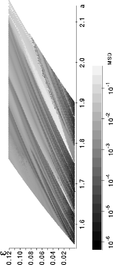
In Fig.10, the MSDs are plotted as functions of the parameter $a$ for several coupling strengths $\epsilon$. Here the system size is chosen to be large enough, to see the behavior of MSD converged in the thermodynamic limit. Two points should be noted here. First, the change of MSD is not monotonic with $a$, but is rather complicated. Second, the change of MSD is complicated with fine structures, which still keep some similarity against the changes of the coupling strength $\epsilon$. For example, a similar but slightly different structure is visible for $a\approx 1.7025$ for $\epsilon=0.01$, $a\approx 1.725$ for $\epsilon=0.015$, and $a\approx 1.73$ for $\epsilon=0.02$. In Fig.11 the parameter dependence of MSD is plotted on the 2-dimensional ($a,\epsilon$) plane. First, regimes with a larger collective motion form tongue-like structures, each of which starts at some point or intervals of parameter $a$ at $\epsilon=0$, and grows with $\epsilon$. Second, the growth of the edge in a tongue-like structure has a nonlinear dependence on the parameters $a$ and $\epsilon$. Third, for almost all parameter values, the MSD of the mean-field remains finite in the thermodynamic limit.

5.2 Effective Nonlinearity

Figure 12: Mean square deviation (MSD) of the mean field dynamics $h_{n}$ are plotted as functions of the effective nonlinearity parameter $A$.

Figure 13: (a)Mean Square Deviation (MSD) of the mean field dynamics is plotted as a function of the effective nonlinearity parameter $A$ and $\epsilon$. The scale shows the value of MSD, where the darkest one corresponds to MSD$\approx 10^{-6}$, and the brightest one to MSD$\approx 10^{-1}$ (see Fig.11).(b)Logistic map bifurcation diagram with the increase of nonlinearity parameter. Horizontal axises are common among two figures.

To see the structure in the parameter space closely, we introduce rescaling of the parameters. For it, we note that each element obeys the following dynamics,

$$x_{n+1}=(1-\epsilon)(1-ax_{n}^{2})+\epsilon h_{n}$$ (6)

where $h_{n}$ is the mean-filed value at time step $n$, which can be considered as a time dependent input to each element. In this map, the nonlinearity is modified by the additional term $h_{n}$. Taking into account of this point, we normalize the variable $x_{n}$ as follows:

$$x_{n}\rightarrow(1-\epsilon+\epsilon h_{n})X_{n}.$$ (7)

Then the logistic map of each element is written as

$$X_{n+1}=1-a(1-\epsilon)(1-\epsilon+\epsilon h_{n}){X_{n}}^{2}$$ (8)

where $a(1-\epsilon)(1-\epsilon+\epsilon h_{n})$ can be regarded as the nonlinearity at time step $n$.

Since the above scaling is time-dependent due to $h_{n}$, we define the effective nonlinearity parameter $A$ as

$$A=(1-\epsilon)(1-\epsilon+\epsilon\langle h\rangle)a.$$ (9)

with the time independent rescaling of $x_{n}$,

$$x_{n}\rightarrow(1-\epsilon+\epsilon\langle h\rangle)X_{n}.$$ (10)

where $\langle h\rangle$ is mean-field average in time,

$$\langle h\rangle=\lim_{t\rightarrow\infty}\frac{1}{t}\sum_{t=0}^{t}h_{n}.$$ (11)

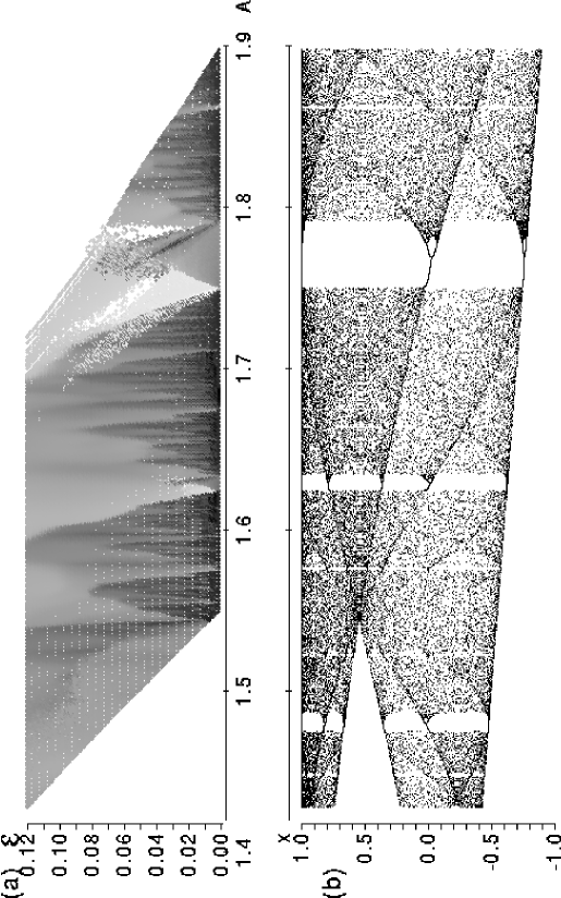
In Fig.12 we have plotted MSD by adopting the effective nonlinearity parameter $A$ instead of $a$. In Fig.13(a) the parameter dependence of MSD is plotted on the 2-dimensional ($A,\epsilon$)-plane. The scaling structure of tongues seems to be much clearer. While the width of each tongue seems to increase roughly linearly with $a$ and $\epsilon$, detailed discussion will be appeared in §7.3.

When the coupling strength $\epsilon$ approaches $0$, each tongue structure corresponds to a window of the single logistic map(Fig.13(b)). For instance, between $A\approx 1.75$ and $A\approx 1.79$ a tongue structure is clearly shown in Fig.13(a), corresponding to the period-3 window of the single logistic map. Although there are countably infinite windows in the parameter space in the logistic map, it is difficult to detect the windows for a longer period numerically. However, it is remarkable that a lot of tongue structures are visible in our model, corresponding to the windows with a longer period.

In each tongue structure, further internal structures exist. For instance, the tongue corresponding to period-3 window of the logistic map between $A=1.75$ and $A\approx 1.79$, has three internal structures, roughly speaking. To understand each inner structure in the tongue, we will study the dynamics of each element and the distribution in the following sections(§6, and §7).

6 Collective Behavior Through Self-Consistent Dynamics

In this section, we briefly describe how the collective motion is formed, especially focusing on the tongue structure.

6.1 Distribution Dynamics

Figure 14: The distribution dynamics is plotted as a function of time. The density of the population is shown with the use of a gray scale. The darker region indicates the high density. The parameters are $a=1.8445$,$\epsilon=0.015$, $N=10^{5}$.

In the limit of $N\rightarrow\infty$, the probability distribution function is defined as follows,

$$\rho_{n}(x)=\lim_{N\rightarrow\infty}\frac{1}{N}\sum_{i}\delta(x-x_{n}(i)).$$ (12)

Oscillation, rather than the fixed point, of the mean field dynamics implies that the probability distribution function does not also remain stationary but depends on time.

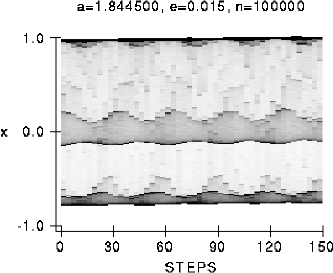
Time series of the probability distribution function by numerical calculation is given in Fig.14. The parameters for the figure $(a=1.8445,\epsilon=0.015)$ belong to the tongue structure in the period 3 window. In this case, since the mean field dynamics has the component of period 3, we plot the figure by every 3 steps to see the slow modulation of $\rho_{n}(x)$. Due to the chaotic oscillation of each element, the distribution function spreads over $x\in[-0.8,1.0]$, but the distribution is not monotonous, and has some structure. In the three regions around $x\approx 1.0,0.0,-0.8$, the population are relatively large. This number “three” corresponds to the period of window which the tongue structure of this motion corresponds to. The number of elements in each three region oscillates in time, and the phase of each oscillation is different from that of the others.

6.2 Formation of Self-Consistent Dynamics

Figure 15: The distribution functions at time $n=0(\ast)$, $20(\bullet)$, $40(\circ)$ are shown.

Figure 16: (a)Time series of the number of elements in the 2 regions, (b)time series of the mean field.$a=1.5449205,\epsilon=0.0005,N=10^{6}$.

Figure 17: Return map of the time series of number of elements in the 2 regions and time series of the mean field, plotted per two steps for even $n$ and odd $n$. $a=1.5449205,\epsilon=0.0005,N=10^{6}$.

It is interesting to view our collective dynamics as an interference between mean field dynamics and individual elements. Before we present a scenario for collective motion, we demonstrate the formation of self-consistent dynamics between the mean field dynamics and individual elements as follows.

For simplicity, we adopt the case, in which the effective nonlinearity parameter $A$ is near the period-2 band merging point(the parameter are $a=1.5449205$, $\epsilon=0.0005$, and the time series and the return map for the parameter are given in Fig.1). The distribution function is given in Fig.15 at every 20 steps. In this case, distribution of elements can be divided into two regions around $x\approx 0.54$. During these 40 time steps the value of distribution function at the left region ($x<0.54$), given in Fig.15(b), decreases with time, while the other region plotted in Fig.15(c) increases with time. Although the change of distribution is quite small, there is a systematic oscillation in the distribution(cf.Fig.20).

Consider a population dynamics of each of the two regions. In Fig.16(a), the population in each region, $N_{L}$, and $N_{R}$ are plotted as a function of time. $N_{L}$ denotes the number of elements in the region smaller than $x\cong 0.54$ in Fig.15, while $N_{R}(=N-N_{L})$ denotes that for larger than $x\cong 0.54$. (The definition for each region is described below in detail.) The population in each region oscillates in time. In Fig.16(b), on the other hand, since the mean field has a component of period two, the time series $h_{n-1}$ and $h_{n}$ are plotted at every two steps. Note that the mean field also oscillates in time with the same period as $N_{R}$, and $N_{L}$, but the phase of the mean field oscillation is different from that of the population dynamics in Fig.16(a).

To see how the mean filed dynamics and the distribution dynamics interfere each other, we construct a return map of above two quantities. Fig.17 is a return map of the distribution dynamics and the mean field dynamics. This figure implies that a self-consistent dynamics is formed as follows,

$$\left\{\begin{array}[]{lll}\tilde{h}_{n}&=&\tilde{h}(\tilde{h}_{n-1},\tilde{N}_{n-1}),\\ \tilde{N}_{n}&=&\tilde{N}(\tilde{h}_{n-1},\tilde{N}_{n-1}),\end{array}\right.$$ (13)

where each $\tilde{h}$ and $\tilde{N}$ is a function of $\tilde{h}_{n}=h_{n-1}-h_{n}$, and $\tilde{N}_{n}=N_{L}-N_{R}$. If the mean field were an external force for each element, the population responds to the mean field value. On the other hand, since population organizes the mean filed dynamics, the collective motion can be described as a self-consistent relation between the population dynamics and the mean field dynamics.

From the above viewpoint, we now demonstrate how the population distribution is modified as the mean field varies slowly.

6.3 Internal Bifurcation in Temporal Domain

Figure 18: Behavior of the third iterate of a logistic map. (a) After tangent bifurcation at three points, and (b)after crisis. Solid lines with arrow indicate iterated trajectories starting from three points

Figure 19: Behavior of the third iterate of the map Eq.(15). In contrast with the case of Fig.18, only one or two regions can attract trajectories. (a)The region around $x=0$ attracts orbits as a region after tangent bifurcation, while the other regions, which are before the tangent bifurcation, cannot attract orbits. (b)Two regions around $x=0$, and $x=-0.8$ attract orbits, while the region around $x=1.0$ can not attract orbits due to the crisis. (c)The region around $x=0$ attracts orbits, while the other regions can not attract orbits due to the the crisis.

Figure 20: Temporal change of $\delta\rho_{n}(x)=\rho_{n}(x)-\langle\rho(x)\rangle$ is plotted by the thick line by magnifying the scale 20 times, while $\delta\rho_{eq,n}^{(2)}(x)=\rho_{eq,n}^{(2)}(x)-\langle\rho(x)\rangle$ is plotted by the thin line, where $\langle\rho(x)\rangle=\lim_{t\rightarrow\infty}\frac{1}{t}\sum_{n=1}^{t}\rho_{n}(x)$. We have plotted them instead of $\rho_{n}(x)$ and $\rho_{eq,n}^{(2)}(x)$ whose change is too small to be visible. Roughly speaking, the population in the region where $\delta\rho_{eq,n}^{(2)}(x)$ is negative is going to the region where $\delta\rho_{eq,n}^{(2)}(x)$ is positive. $\delta\rho_{eq,n}^{(2)}(x)$ changes qualitatively at $n=12$ (c). $a=1.5449176,\epsilon=0.0005,N=10^{6}$.

If the mean field were an external force for each element, it could be regarded that each element follows the logistic map with external force. This is valid if the mean field varies slowly. In this case, the motion of equation for the $i$’th element is given by

$$x_{n+1}(i)=F_{n}(x_{n}(i)),$$ (14)

with

$$F_{n}(x)=(1-\epsilon)(1-ax^{2})+\epsilon\langle h\rangle+\epsilon\cdot\delta h_{n},$$ (15)

where $\delta h_{n}$ is difference from $\langle h\rangle$, i.e., $h_{n}=\langle h\rangle+\delta h_{n}$.

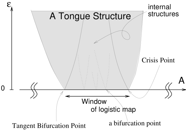
If we took $\delta h_{n}$ out of consideration, the dynamics of each element would be same as the logistic map with the nonlinearity parameter $A=a(1-\epsilon)(1-\epsilon+\epsilon\langle h\rangle)$. Since in the previous section (§5) each tongue structure has good correspondence with a window of the logistic map, here we especially focus on the window structure of the logistic map. In the case of the logistic map, the period $p$ window starts at the tangent bifurcation point of the $p$’th iterate of the map, and then the period doubling bifurcation proceeds with the increase of $a$, until the window ends up by crisis(see Fig.18). Note that for a period $p$ window tangent bifurcation or crisis occurs at $p$ points of $x$ at the same value of $A$. In this case, since Eq.(15) has an invariant measure, the probability distribution in each of $p$ pieces of regions is equivalent.

Take $\delta h_{n}$ in Eq.(15) into account as an external force. The bifurcation of a logistic map with time dependent external force has a crucial difference from usual bifurcation of the logistic map. In Fig.19, examples of the third iterates of the map with external force are shown. In Fig.19(a) a region around $x\approx 0$ crosses $y=x$, while two regions around $x\approx 0.95$ and $x\approx-0.75$ do not cross $y=x$. In Fig.19(b)(c), while three regions cross $y=x$, one or two of the regions are collapsed by crisis.

In general, consider the case of period $p$ window with external force. Since the tangent bifurcation or crisis of $p$ points occurs at a different value of $A$, the number of divided attractors can be changed with $A$. Even if trajectories are attracted into $p$ distinct regions, the probability distribution in each region is not equivalent.

As we have seen in the previous subsection(§6.2), slow modulation of the mean field leads to the dynamics of the distribution of population. With the slow modulation of $\delta h_{n}$ in time, behavior of each element also changes. In other words, with the change of $\delta h_{n}$, bifurcation can occur in the effective map for each element,

$$F^{(p)}_{n}=F_{n+p-1}\circ F_{n+p-2}\circ\cdots\circ F_{n+1}\circ F_{n},$$ (16)

which is the $p$’th iterate of the map Eq.(15). Since $\delta h_{n}$ changes temporally, such bifurcation occurs temporally. To distinguish from the notion of bifurcation in parameter space, such bifurcation is called as “internal bifurcation”. While the notion of “internal bifurcation” indicates the slow modulation of the effective map Eq.(16), since time dependence of $\delta h$ induces asymmetry in this effective map, as we have shown in the previous paragraph, the dynamics of the mean field has component of period $p$ motion. This is why we have plotted the time series of the mean field and the probability distribution function at every $p$ steps.

To characterize the effective map at every $p$ time steps, we introduce the invariant measure $\rho_{eq,n}^{(p)}(x)$ determined from the Perron-Frobenius equation,

$$\rho_{eq,n}^{(p)}(x)=\int_{-1}^{1}\rho_{eq,n}^{(p)}(y)\delta(x-F_{n}^{(p)}(y)))dy.$$ (17)

If the mean field changes slowly, we can approximately regard our GCM dynamics as relaxation process of $\rho_{n}(x)$ to $\rho_{eq,n}^{(p)}(x)$. In each time step, elements follow the effective map Eq.(16) so that the distribution function $\rho_{n}(x)$ is going to be relaxed. The elements in the region where $\rho_{eq,n}^{(p)}(x)-\rho_{n}(x)<0$ are going to the region where $\rho_{eq,n}^{(p)}(x)-\rho_{n}(x)>0$. As a result $\rho_{n}(x)$ is going to relax into $\rho_{eq,n}^{(p)}(x)$.

On the other hand, the mean field is derived as, $h_{n}=\int f(x)\rho_{n}(x)dx$. Relaxation of $\rho_{n}(x)$ can lead the mean field to a certain critical value, at which the internal bifurcation occurs in the effective map Eq.(16). For instance, small difference of the mean field induces one point in the effective map to be tangential to $y=x$, or one region to be collapsed by crisis. As a result, the nature of the invariant measure $\rho_{eq,n}^{(p)}(x)$ of the effective map changes qualitatively.

With this internal bifurcation, the distribution $\rho_{n}(x)$ is not actually relaxed to $\rho_{eq,n}^{(p)}(x)$, because 1) the velocity of change $\rho_{n}(x)$ is finite, and 2) the relaxation of $\rho_{n}(x)$ makes $\rho_{eq,n}^{(p)}(x)$ to be changed qualitatively. Consequently $\rho_{n}(x)$ oscillates in time. This is a qualitative explanation why the mean field does not approach a fixed point at the thermodynamic limit.

Let us look back to the example in the subsection §6.2 and try to describe the dynamics along the above scenario. Population distribution function $\rho_{n}(x)$ at time step $n$ is plotted with the solid line in Fig.20(and see the caption in it). Since the effective nonlinearity parameter $A$ is near the band merging point of the logistic map, it is useful to define the two regions as follows. The effective map given by the second iterate of map,

$$F_{n}(F_{n-1}(x))=(1-\epsilon)f((1-\epsilon)f(x)+\epsilon h_{n-1})+\epsilon h_{n},$$ (18)

has three unstable fixed points and the middle of these points is denoted by $x_{n}^{*}$. $R$ and $L$ denote the region where $x>x_{n}^{*}$ and $x<x_{n}^{*}$ respectively. (Based on this definition, we have calculated the number of elements in the two regions, from which Fig.17 in the subsection §6.2 is obtained.)

In this parameter, if the unstable fixed point of the mean field solution were realized, these two regions collapse due to the crisis. Hence, these two region are unstable. (In the bellow “stable” or “unstable” means that a region, $R$ or $L$, can attract trajectories or not.) As we have discussed above, however, dynamics of the mean field modulates the effective map Eq.(18), and then, for this parameter regime, there are three cases: 1) $R$ region is stable and $L$ is unstable, 2) $R$ region is unstable and $L$ is stable, or 3) both $L$ and $R$ regions are unstable.

The effective map Eq.(18) can be characterized as invariant measure of effective map $\rho_{eq,n}^{(2)}(x)$, which depends on the mean field value. The stability in each region can be seen by the strength of $\rho_{eq,n}^{(2)}(x)$. The thin lines in Fig.20 are $\rho_{eq,n}^{(2)}(x)$(see the caption in Fig.20). In Fig.20(a), $R$ region is unstable and $L$ region is stable at $n=1$ as is shown by $\rho_{eq,n}^{(2)}(x)$. Since $\rho_{n}(x)$ is going to relax to $\rho_{eq,n}^{(2)}(x)$, the elements in $R$ region moves to $L$ region as is shown in Fig.20(a) and (b). Indeed the number of elements decreases in $R$ region and increases in $L$ region in Fig.16(a) and (b). This change of $\rho_{n}(x)$ continues until the modulation of the mean field induces crisis of $L$ region at $n=12$ in Fig.20(c). By this destabilization of $L$ region, elements in $L$ region move to $R$ region so as to relax the distribution $\rho_{n}(x)$ to $\rho_{eq,n}^{(2)}(x)$ in Fig.20(d) and (e), until the next crisis leads to the structure of Fig.20(a), giving a flow from $R$ region to $L$.

To sum up, distribution function $\rho_{n}(x)$ changes slowly so as to relax to $\rho_{eq,n}(x)$ and the distribution $\rho_{n}(x)$ changes until the modulation of the mean field induces internal bifurcation structure to change qualitatively. In this example, qualitative change in internal bifurcation is due to local crisis. By the change of stability in two regions, $\rho_{n}(x)$ relaxes to a different region. With the repetition of this stability change the mean field oscillates quasi-periodically. This mechanism of the stability change in each band holds for any period-p band(window) regime where elements are attracted to and repelled from each band region successively with the internal bifurcation giving rise to crisis.

7 Bifurcation of Collective Motion

7.1 Bifurcation of Tongue Structures

Figure 21: Ratio of the time steps, in which the two regions are both stable(“stable+stable”), one of the regions are stable(“unstable+stable”), and the two regions are both unstable(“unstable+unstable”). $\epsilon=0.0005$, $N=10^{7}$. The instability is due to the crisis bifurcation in internal bifurcation.

Figure 22: Mean square deviation (MSD) of the mean field distribution with the increase of $\epsilon$ plotted as a function of the effective nonlinearity parameter $A$. The region corresponds to the period-2 tongue structure. $A_{0}$ denotes the band merging point (crisis bifurcation point of 2-band) of the logistic map ($A_{0}=1.543689012692076$).

As we have seen in Fig.20 in the previous section (§6.3), one of the two regions in the second iterate of the effective map Eq.(18) is collapsed due to the crisis at some time steps and such a region changes in time. With the increase of $a$, the time interval of crisis bifurcation becomes longer. In Fig.21, the ratio of the time interval, during which one of the two regions is unstable and the other is stable, the two regions are both unstable, and the two regions are both stable, are plotted with the change of the nonlinearity parameter $a$. For $a\leq 1.5449173$, crisis bifurcation never occurs both in the two regions, while for $a>1.5449173$, the time interval of crisis is getting longer. For the parameter beyond $a=1.5449212$, the two regions is collapsed due to the crisis bifurcation all time steps. Hence, the period-2 tongue structure starts at the parameter, where one of the two regions in the second iterate of the effective map Eq.(18) is collapsed due to the crisis at some time steps at $a\cong 1.5449173$, and ends up at the parameter where both the two regions collapse due to the crisis all the time at $a\cong 1.5449212$.

Consider an internal bifurcation condition of Eq.(16) (for instance, crisis bifurcation or tangent bifurcation in each element.). While for $\epsilon=0$ the bifurcation condition holds at only one point in the nonlinearity parameter, for finite $\epsilon$, due to the oscillation of the mean field, the internal bifurcation condition is satisfied for some steps within some interval $A_{small}(\epsilon)<A(\epsilon)<A_{large}(\epsilon)$ in the parameter space. Hence, the edge of a tongue structure, corresponding to a periodic window of logistic map, starts from tangent bifurcation and crisis bifurcation point at $\epsilon=0$, and each line constitutes the parameter $A$ and $\epsilon$, where each bifurcation condition holds at some time steps(Fig.22 for period-2 tongue structure). Scaling the width of tongue structure will be discussed lated (in §7.3).

7.2 Bifurcation in a Tongue Structure

Figure 23: (a)Mean square deviation and (b)rotation number of the mean field dynamics are plotted as a function of $a$. For the parameter $a=1.6962$, $1.69755$, and $1.69844$ indicated in the figure (a), see Fig.3 and Fig.24

Figure 24: Invariant measure of the effective map Eq.(19) $\rho_{eq,n}^{(7)}(x)$ is plotted as a function of time. The horizontal axis is time and the vertical axis is $x$. In this figure, the region with $\rho_{eq,n}^{(7)}(x)>0$ is plotted by a solid line. When the whole the region is filled by a line, none of the seven regions of the map Eq.(19) cross with $y=x$, and all the regions are connected as a single attracting set. In (a) and (b) some of the seven regions of the map Eq.(19) cross with $y=x$, while the other regions do not. In (c), on the other hand, all seven regions of the map Eq.(19) cross with $y=x$, while some of the seven regions are destabilized by crisis. The parameters correspond to that of Fig.3.

Even within the same tongue structure, we can observe different types of collective motion. With the change of the parameter $a$ and $\epsilon$, the collective dynamics shows a kind of bifurcation. Since the collective dynamics remains high-dimensional, it is not described as a standard bifurcation in low-dimensional dynamical systems. Here we study a mechanism of such change in the collective dynamics.

In Section 3, it is shown that slight increase in $a$ induces the qualitative change of collective dynamics (Fig.3). To see this quantitatively, it may be convenient to measure the rotation number of collective dynamics. In Fig.23, the rotation number is plotted as a function of $a$. In the regime plotted in the figure (i.e., between $a\in[1.69614,1.69847]$ with $\epsilon=0.008$), period-seven tongue structure is observed. Roughly speaking this period-seven tongue region is divided into 3 regimes in Fig.23, $a\in[1.69614,1.6975]$, $a\in[1.6975,1.698]$ and $a\in[1.698,1.69847]$. Typical example for each regime are shown in Fig.3.

To see the mechanism of the difference of dynamics in these parameter region, it may be useful to adopt the invariant measure $\rho_{eq,n}^{(7)}(x)$ of the effective map,

$$F^{(7)}_{n}=F_{n+6}\circ F_{n+5}\circ\cdots\circ F_{n+1}\circ F_{n},$$ (19)

as we have already introduced in Section 6. In Fig.24, three examples of $\rho_{eq,n}^{(7)}(x)$ are plotted as a function of time, corresponding to the three regimes mentioned above. In Fig.24(a), seven distinct regions are stabilized successively. For this parameter, the effective nonlinearity parameter $A$ is close to, but smaller than, the tangent bifurcation point of the period seven window in the logistic map. Therefore if the fluctuation of the mean field were ignored, none of the seven regions would be stabilized because the seventh iterate of the logistic map Eq.(19) does not cross with $y=x$. With the mean field dynamics, on the other hand, the effective map Eq.(19) is modified to cross with $y=x$ at a few regions where $\rho_{eq,n}^{(7)}(x)>0$(for instance between $n=2000$ and $2100$ in Fig.24(a)). In Fig.24(a), two or three regions are stabilized. After some duration, these regions come to be destabilized again by crisis (for instance at $n\approx 2100$ in Fig.24(a)). After the crisis $\rho_{eq,n}^{(7)}(x)$ spreads over the whole region because none of the seven regions of the map Eq.(19) cross with $y=x$. Then stabilized regions switch to different positions. This process continues successively.

When the parameter $a$ is increased, the number of regions stabilized by the tangent bifurcation of the map Eq.(19) is increased (Fig.24(b)). In Fig.24(b), 5,6,or 7 regions are stabilized successively. This corresponds to the second regime in Fig.23.

With the further increase of $a$, all the seven regions of the map Eq.(19) always cross with $y=x$, while some of these seven regions are destabilized by crisis(Fig.24(c)), as we have shown in section 6. With the increase of $a$, time duration of crisis in each seven region is increased, and all the seven regions start to be destabilized by crisis at the same time step. Then this tongue structure ends up and collective dynamics in the p7 tongue structure is collapsed (at $a=1.69847$). Then the amplitude of mean-filed dynamics is reduced smaller to about $1\over 10$(see Fig.23).

Although we have explained the bifurcation in the internal tongue structure for the period-7 case, this kind of bifurcation structure is common to a band region in any period. For instance, in Fig.13(a) with the period-3 tongue structure (starting from $A\in[1.75,1.79032]$ at $\epsilon=0.0$) and in the period-5 tongue structure(starting from $A\in[1.6244,1.6333]$ at $\epsilon=0.0$), similar bifurcation structure can be observed, where the change in the number of coexisting stable regions makes such bifurcation structure.

7.3 Scaling of Tongue Structures

Figure 25: Scaling relation of tongue structure for period-2 (a), period-3(b), and period-5(c). $\epsilon\delta h$ are plotted as functions of $\delta A$, where $\delta h=\sqrt{\mbox{MSD}}$ and $\delta A$ indicate the deviation from the band merging point($A=1.543689012692076$)(Fig.(a)), the crisis bifurcation point of period-3 window($A=1.790327491999345$)(Fig.(b)), and the crisis bifurcation point of period-5 window($A=1.633358703691276$)(Fig.(c)) of the logistic map, respectively. Line in each figure is proportional to $\delta A$. Hence, the edge of $A$ in a tongue structure varies linearly with $\epsilon\delta h$. The width of a tongue structure increases proportional to $\epsilon\delta h$.

Figure 26: The maximum and next maximum value of $\delta h=\sqrt{\mbox{MSD}}$ in each tongue structure are plotted. They are obtained by sampling the data of MSD by changing $A$ in each tongue with for each $\epsilon$.

As we have shown in §5.2, the width in the parameter $A$ of each tongue increases with $\epsilon$ (see Fig.13(a)). Here, we discuss the scaling of each tongue structure.

In general, the effective map for each element is given by

$$F^{(p)}_{n}=F_{n+p-1}\circ F_{n+p-2}\circ\cdots\circ F_{n+1}\circ F_{n},$$ (20)

with $F_{n}(x)=(1-\epsilon)(1-ax^{2})+\epsilon h_{n}$. By adopting the effective nonlinearity parameter $A$ and rescaling of $x_{n}(i)$, which we have introduced in §5.2, $F_{n}(x)$ may be transformed into

$$F_{n}(x)=1-Ax^{2}+{\epsilon\cdot\delta h_{n}\over 1-\epsilon+\epsilon\langle h\rangle},$$ (21)

where $\delta h_{n}=h_{n}-\langle h\rangle$. As we have mentioned adobe, an internal bifurcation condition, e.g. crisis bifurcation, and tangent bifurcation, is satisfied for some steps within some parameter interval $A_{small}(\epsilon)<A(\epsilon)<A_{large}(\epsilon)$. (Indeed this region corresponds to each tongue structure). Roughly speaking, $\delta h_{n}$ varies in time within $[-\sqrt{\mbox{MSD}}:\sqrt{\mbox{MSD}}]$ for a given parameter. Thus, the minimum and maximum parameter of $A$ in a tongue structure is a function of $-\epsilon\sqrt{\mbox{MSD}}$ and $+\epsilon\sqrt{\mbox{MSD}}$ respectively, i.e., $A_{small}$ and $A_{large}$ are given as

$$A_{small}(\epsilon)=A_{0}+A_{1}(-\epsilon\sqrt{\mbox{MSD}})+O\left((\epsilon\cdot\sqrt{\mbox{MSD}})^{2}\right),$$

$$A_{large}(\epsilon)=A_{0}+A_{1}(+\epsilon\sqrt{\mbox{MSD}})+O\left((\epsilon\cdot\sqrt{\mbox{MSD}})^{2}\right).$$ (22)

where $A_{0}$ is a bifurcation parameter of the logistic map, and $A_{1}$ is positive constant.

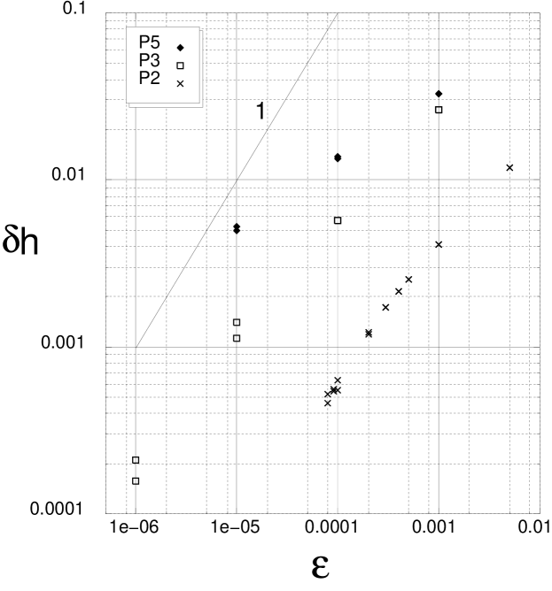
For instance, the band merging point of logistic map separates into two lines as is shown in Fig.22. In Fig.25, tongue structures around the parameter $A$ at the crisis bifurcation point of the period-2 window(band merging point), period-3 window, and period-5 window are shown. The linear scaling relation with $\epsilon\sqrt{\mbox{MSD}}$ is clearly seen as to the change of $A_{small}$ and $A_{large}$. Thus the width of the tongue structure grows linearly with $\epsilon\cdot\delta h$.

To obtain the scaling of the tongue structure as a function of $\epsilon$, we have to know the dependence of MSD on $\epsilon$. In Fig.26, the growth of square root of the MSD of the mean field dynamics in a tongue structure with the coupling strength $\epsilon$ is shown for several tongue structures. While it has been pointed out that the amplitude of the mean field dynamics may grow linearly with $\epsilon$ for globally coupled logistic map[8, 19], Fig.26 indicates a possibility that there is a deviation from the linear scaling with $\epsilon$ for the amplitude of the mean field. It should be noted that while we have payed attention mainly to tongue structures relevant to windows of the logistic map, in the reference[19] such window structures in the logistic map are out of consideration. In other words, they have focused on the collective dynamics arising from completely chaotic dynamics in the logistic map. Note also that our analysis is based on the rescaled nonlinearity parameter $A$, while the studies in the references [8, 19] are based on $a$. Possible distinction between the collective motions originated in chaos and window will be discussed in §9 again.

8 Hysteresis, Multiple Attractors, and Coexistence of Different Types of Motion

Figure 27: Time series of elements. Elements are accumulated to three bands. In the figure time series of 100 elements out of $10^{5}$ are plotted at every three steps. A lot of attractors are realized depending on the population ratio to each band, while elements are desynchronized each other. The parameters are $a=1.85$, $\epsilon=0.018$, $N=10^{5}$.

Figure 28: Hysteresis curve observed by increasing or decreasing progressively the control parameter $a$ while keeping the final state of a simulation at given $a$ as the initial condition for the neighboring value $a-\delta a(\times)$ and $a+\delta a(+)$. $\epsilon=0.008$. The MSD calculated starting from a random initial condition are also plotted ($\diamond$).

Figure 29: Time series and return map for two attractors in Fig.28. The parameters are $a=1.69855$, $\epsilon=0.008$.

Figure 30: Time series of elements for the same parameter in Fig.27 starting from different initial condition. In contrast with Fig.27, elements spread over $x$. The mean field dynamics for this time series shows quasi-periodic-like motion. Time series are plotted for 100 elements at every three steps. The parameters are $a=1.85$, $\epsilon=0.018$, $N=10^{5}$.

Figure 31: Return maps of element motions to show the coexistence of different kinds of motions. $\mbox{P}_{1}$(circled) and $\mbox{P}_{2}$ represent the element motion belonging to a different band in the dynamics, respectively. Two kinds of motions (P₁, and P₂) coexist. $\mbox{P}_{1}:\mbox{P}_{2}$ in each figure indicates the number of population in each group. With the change of ratio, two kinds of motions are varied. The parameters are $a=1.88,\epsilon=0.04,N=10^{4}$.

Even if the control parameters are same, depending on its initial condition, there can exist more than one attractors of the collective motion.

Most straightforward examples of multiple attractors are given with the use of band splitting. At same parameter region, while there is no mutual synchronization, elements are accumulated to few bands and never change their band(Fig.27). Therefore, a lot of attractors are realized depending on the population ratio to each band, as long as stability conditions are satisfied. For instance, In Fig.27, elements are accumulated into three bands. (see e.g. [14] for the case with a tent map).

The next example of multiple attractors is concerned with hysteresis phenomena of collective motion, which can be observed at the edge of the tongue structure in the parameter space. In Fig.28, hysteresis curve of MSD is observed by increasing or decreasing the control parameter $a$ with the use of the final state of a simulation at the previous value of $a$ as the next initial condition. Thus in $a\in[1.69848:1.69858]$, at least two different attractors of the collective motion coexist. In Fig.29, time series and return map for each attractor are shown. Note that, in this case there is no separated bands in contrast with the previous examples.

The third example of multiple attractors, one attractor has a band structure (Fig.27) and the other not (Fig.30). For the former attractor, elements are accumulated in a few bands, while for the latter elements spread over whole range of $x$. Moreover for the former type, there exists a lot of attractors with a different ratio of population in each band, as in the first example.

Another important topic related to the multiple attractor is the coexistence of different kinds of element motions. When the elements are accumulated into few bands, depending on the ratio of population in bands, the motion of elements in each band is different. In Fig.31, two kinds of element motions are plotted for attractors with different population splitting ratio into bands. At this parameter, there is a three-band structure, and elements are accumulated into two groups of these three bands. Note that while these groups are similar to clusters (cf. [6]), but the value of elements $x_{n}(i)$ in each group are different each other. Depending on the ratio of population in the two groups, two kinds of element motion coexist. Relevance of such coexistence to the problem of cell differentiation is discussed in[31].

9 Summary and Discussions

Figure 32: Schematic diagram of tongue bifurcation structure. Regions that grow from a bifurcation point of the logistic map constitute a tongue structure. See §7

In the present paper, we have studied the collective motion in desynchronized state of globally coupled logistic maps. It is shown that the motion with a much longer time scale and lower dimension can emerge in macroscopic dynamics, such as the mean field dynamics. The amplitude of collective motion (mean square deviation of the mean field distribution) is studied by changing the nonlinearity parameter $a$ and the coupling strength $\epsilon$. By introducing the effective nonlinearity parameter $A$ with rescaling of $x_{n}(i)$, tongue structure has been detected in ($A,\epsilon$)-plain. Each tongue structure corresponds to a periodic window of logistic map.

Focusing on the tongue structure, we have demonstrated how such a collective motion emerges. Self-consistent dynamics between the mean field dynamics(macroscopic dynamics) and each element(microscopic dynamics) is found to be formed, so that such a collective motion is possible. This self-consistent dynamics is formed by the following circulation: accumulation of elements into some regions leading to the change in the mean field dynamics, which introduce the stability change of the the regions, and flow of elements into a different region, which, again….. This gives internal bifurcation in elements and in time.

The bifurcation is also seen in the parameter space. Since the nature of the internal bifurcation varies with the nonlinearity parameter $a$ in a tongue structure, the number of coexisting regions in $x$ changes, which makes the collective motion qualitatively different. Hence, in a tongue structure, different kinds of collective motions have been observed. (A schematic figure of tongue structure is presented in Fig.32).

With the increase of the coupling strength $\epsilon$, each tongue structure grows in proportion to $\epsilon\cdot\delta h$, where $\delta h$ is the amplitude of the mean field variation. Hence the width of each tongue increases with $\epsilon^{2}$ if $\delta h\propto\epsilon$. In contrast with earlier studies[8, 19] supporting this linear scaling, however, our calculation suggests that the scaling may obey a different power law.

Existence of multiple attractors with a different collective motion have also been reported. This means that there can be non unique self-consistent dynamics between microscopic and macroscopic motion. It should be noted that in the case of the multiple attractors, since the average mean field is clearly different by attractors, they take different values of the effective nonlinearity parameter $A$, and are distinguishable clearly in the ($A,\epsilon$)-plain.

Our tongue structure is based on the windows that exist in the logistic map. Since the window exists in any neighborhood in the parameter space of the logistic map and the width of the tongue structure increases with the coupling $\epsilon$, the tongue structure is expected to occupy a relatively large region in the parameter space. This is one of the reasons why we have focused our attention on the collective behavior in the tongue structures. Still, we have to note that there is a positive measure in the parameter space of the logistic map, corresponding to chaos. Hence, at least at small coupling regime in our GCM, there are parameters with a positive measure which do not belong to any tongue structure. Indeed, we have observed that the amplitude of the mean-filed variation drops less than to $1/10$(see Fig.12), at the parameter where the tongues structure disappears. Although no clear structure in the return map is detected there, this motion again has some hidden coherence and is distinguishable from noise. Analytical estimate of the mean field dynamics by S. V. Ershov, et al.[19] is expected to correspond to such chaos-originated regime. However, we need further study to clarify the mechanism of the collective dynamics there, and characterize the high-dimensional chaos.

While in the desynchronized state elements are completely desynchronized each other and all the Lyapunov exponents are positive, for some parameter regime, some kind of predictability may emerge in the macroscopic variables. However, since low-dimensional ($O(1)$) collective dynamics has not been observed, microscopic and macroscopic dynamics are not separated completely. This is why we need a self-consistent description between microscopic variable ($x_{n}(i)$) and the mean-field. On the other hand, it might be also important to study how such characteristics of the collective motion are reflected on $N$-dimensional phase space structure, or on microscopic quantities, such as the Lyapunov spectrum. With such study, the mechanism for our collective motion must be clearly distinguishable from the self-organization mechanism[32] or the slaving principle [33]. Although we have presented a heuristic way to extract such self-consistent dynamics in the present paper, it is hoped that a systematic method to characterize the (high-dimensional) collective motion will be developed in future.

References

- [1] S. Watanabe, S. H. Strogatz, Constants of motion for superconducting Josephson arrays, Physica D 74 (1994) 197-253.; and references therein.
- [2] C. Bracikowski, R. Roy, Chaos in a multimode solid-state laser system, Chaos 1 (1991) 49; F. T. Arecchi, Rate processes in nonlinear optical dynamics with many attractors, Chaos 1 (1991) 357.
- [3] Ad Aertsen, M. Erb, G. Plam, Dynamics of functional coupling in the cerebral cortex: an attempt at a model-based interpretation, Physica D 75 (1994) 103-128.; and references therein.
- [4] E. P. Ko, T. Yomo, I. Urabe, Dynamics clustering of bacterial population, Physica D 75 (1994) 81-88.; K. Kaneko, T. Yomo, Cell division, differentiation and dynamic clustering, Physica D 75 (1994) 89-102.
- [5] P. J. Godin, T. G. Buchman, Uncoupling of biological oscillators: A complementary hypothesis concerning the pathogenesis of multiple organ dysfunction syndrome, Crit. Care. Med. 24 (1996) 1107-1116.; T. G. Buchman, Physiological Stability and Physiologic State, J. Trauma 41 (1996) 599-605.
- [6] K. Kaneko, Clustering, Coding, Switching, Hierarchical Ordering, And Control In A Network Of Chaotic Elements, Physica D 41 (1990) 137-172.
- [7] K. Kaneko, Globally Coupled Chaos Violates the Law of Large Numbers, Phys. Rev. Lett. 65 (1990) 1391.
- [8] K. Kaneko, Mean field fluctuation of a networks of chaotic elements, Physica D 55 (1992) 368-384.
- [9] G. Perez and H.A. Cerdeira, Instabilities and nonstatistical behavior in globally coupled systems, Phys. Rev. A 46 (1992) 7492.
- [10] H. Chaté, P. Manneville, Collective Behaviors in Spatially Extended Systems with Local Interactions and Synchronous Updating, Prog. Theor. Phys. 87 (1992) 1.
- [11] G. Perez, S. Sinha, H. A. Cerdeira, Order in the turbulent phase of globally coupled maps, Physica D 63 (1993) 341-349.
- [12] A. S. Pikovsky and J. Kurths, Do Globally Coupled Maps Really Violate the Law of Large Numbers?, Phys. Rev. Lett. 72 (1994) 1644; A.S. Pikovsky and J. Kurths, Collective behavior in ensembles of globally coupled maps, Physica D 76 (1994) 411-419.
- [13] W. Just, Bifurcations in Globally Coupled Map Lattices, J. Stat. Phys. 79 (1995) 429.
- [14] K. Kaneko, Remarks on the mean field dynamics of networks of chaotic elements, Physica D 86 (1995) 158-170.
- [15] S. V. Ershov, A. B. Potapov, On Mean Field Fluctuations In Globally Coupled Maps, Physica D 86 (1995) 532-558.
- [16] S. Morita, Bifurcation in globally coupled chaotic maps, Phys. Lett. A 211 (1996) 258-264.
- [17] H. Chaté, A. Lemaitre, Ph. Marcq, P. Manneville, Non-trivial collective behavior in extensively-chaotic dynamical systems: an update, Physica A 224 (1996) 447-457.
- [18] T. Shibata, K. Kaneko, Heterogeneity Induced Order in Globally Coupled Chaotic Systems, Europhysics Letters 38(6) (1997) 417–422.
- [19] S. V. Ershov, A. B. Potapov, On Mean Field Fluctuations In Globally Coupled Logistic-Type Maps. Physica D 106 (1997) 9-38.
- [20] N. Nakagawa, T. Komatsu, Collective motion occurs inevitably in a class of populations of globally coupled chaotic elements, Phys. Rev. E (1998) in press.
- [21] T. Chawanya, S. Morita, On the bifurcation structure of the mean-field fluctuation in the globally coupled tent map systems. Physica D, in press.
- [22] K. Kaneko, Period-doubling of kink-antikink patterns, quasi-periodicity in antiferro-like structures and spatial intermittency in coupled logistic lattice –toward a prelude to a “field theory of chaos”—, Prog. Theor. Phys. 72 (1984) 480; Pattern dynamics in spatiotemporal chaos, Physica D 34 (1989) 1; Simlulating Physics with Coupled Map Lattice, Formation, Dynamics, and Statistics of Patterns, K. Kawasaki, A. Onuki, and M. Suzuki eds. (World Scientific. Singapore, 1990); Theory and Applications of Coupled Map Lattices, K. Kaneko, ed. (Wiley, New York, 1993).
- [23] K. Okuda, Variety and generality of clustering in globally coupled oscillators, Physica D 63 (1993) 424-436.
- [24] N. Nakagawa and Y. Kuramoto, Collective chaos in a population of globally coupled oscillators, Prog. Theor. Phys. 89 (1993) 313.
- [25] K. Kaneko, Dominance of Milnor Attractors and Noise-induced Selection in a Multi-attractor System, Phys. Rev. Lett,78 (1997) 2736-2739.
- [26] K. Ikeda, K. Matsumoto, and K. Otsuka, Maxwell-Bloch turbulence, Prog. Theor. Phys. Suppl. 99 (1989) 295; I. Tsuda, Chaotic itinerancy as a dynamical basis of Hermeneutics in brain and mind, World Futures 32 (1992) 313.
- [27] N. Nakagawa and Y. Kuramoto, From collective oscillations to collective chaos in a globally coupled oscillator system, Physica D 75 (1994) 74-80.
- [28] M. Chabanol, V. Hakim, W. Rappel, Collective chaos and noise in the globally coupled complex Ginzburg-Landau equation, Physica D 103 (1997) 273-293.
- [29] Y. Kuramoto, Surikagaku 408 (1997) 5, in Japanese.
- [30] P. Grassberger, I. Procatia, Characterization of strange attractors, Phys. Rev. Lett.50(1983)346; Measuring the strangeness of strange attractors, Physica D 9 (1983) 189.
- [31] C. Furusawa and K. Kaneko, Emergence of Rules in Cell Society: Differentiation, Hierarchy, and Stability, Bull. Math. Biol., in press.
- [32] G. Nicolis, I. Prigogine, Self-organization in nonequilibrium systems, (John Wiley Sons, Inc. 1977).
- [33] H. Haken, Synergetics, (Springer-Verlag Berlin Heidelberg, 1976).
- [34] T. Shibata, K. Kaneko, (1998), in preparation.