Low dimensional travelling interfaces in coupled map lattices

Abstract

We study the dynamics of the travelling interface arising from a bistable piece-wise linear one-way coupled map lattice. We show how the dynamics of the interfacial sites, separating the two superstable phases of the local map, is finite dimensional and equivalent to a toral map. The velocity of the travelling interface corresponds to the rotation vector of the toral map. As a consequence, a rational velocity of the travelling interface is subject to mode-locking with respect to the system parameters. We analytically compute the Arnold’s tongues where particular spatio-temporal periodic orbits exist. The boundaries of the mode-locked regions correspond to border-collision bifurcations of the toral map. By varying the system parameters it is possible to increase the number of interfacial sites corresponding to a border-collision bifurcation of the interfacial attracting cycle. We finally give some generalizations towards smooth coupled map lattices whose interface dynamics is typically infinite dimensional.

Keywords: Coupled map lattices, travelling waves, mode-locking, circle map, rotation number, bifurcation.

I Introduction

Coupled map lattices (CML) where introduced by Kaneko [1983, 1984] as a paradigm for the study of spatio-temporal complexity such as turbulence [Kaneko, 1986, 1989, Beck 1994], convection [Yanagita & Kaneko, 1993], open flows [Willeboordse & Kaneko 1995, Kaneko 1985], patch population dynamics [Hassell et al., 1995, Sole & Bascompte 1995], etc. An interesting spatio-temporal feature is the emergence of coherent travelling structures [Kaneko 1992, 1993] along the lattice. In this paper we use a simple example of a piece-wise linear one-way CML with two superstable basins in order to restrict the front dynamics to a finite dimensional system. At the beginning of Sec. 2 we recall some features in a particular region of the parameter space where the travelling interface consist of a single site. The dynamics in this case can be reduced to a one-dimensional map of the circle. The velocity of the travelling interface is computed by means of the rotation number of the circle map and thus the mode-locking regions of the velocity with respect to the system parameter are computed analytically. Later in Sec. 2 we perform an equivalent approach for the case of a 2 sites travelling interface. Here the dynamics of the travelling interface can be reduced to a two-dimensional toral map whose rotation vector gives the travelling velocity. We give a method for computing the mode-locking regions in this case. In Sec. 3 we present the Arnold’s tongues for higher dimensional interfaces and show the bifurcation diagram as the number of sites in the interface is increased. Finally we give some comments on the generality of our results for generic bistable local maps whose attractors do not possess superstable basins and thus their corresponding travelling interface is typically infinite dimensional.

A CML is a dynamical system with discrete space, discrete time and continuous state space. We could think of CMLs as a generalization of cellular automata whose state space is discrete [Chate & Manneville, 1989, 1990]. Consider a one-dimensional collection of cells labeled by the integer index $i$ and with dynamical variable $x_{t}(i)$ at time $t$. The lattice could be infinite or finite with periodic or fixed boundary conditions. For the present study the particular choice of lattice is not crucial since we deal with the propagation of finite dimensional localized structures with spatio-temporal periodicity. Therefore, for the numerical experiments, it suffices that the lattice is large enough to enclose the localized front for a whole period. The CML dynamics consists of two independent stages: the local dynamics and the coupling dynamics. The former is the application of the one-dimensional local map $f_{i}(x)$ to every site and the latter couples the dynamics by means of a weighted sum over a neighbourhood $\nu_{i}$:

$$\begin{array}[]{rcl}x_{t}(i)&\overrightarrow{\quad\rm{local}\quad}&f_{i}(x_{t}(i))\\[12.91663pt] &\overrightarrow{\quad\rm{coupling}\quad}&x_{t+1}(i)=\sum_{\nu_{i}}{\varepsilon_{\nu_{i}}f_{\nu_{i}}(x_{t}(i))},\end{array}$$ (1)

where the coefficients $\varepsilon_{\nu_{i}}$ determine the type of coupling interaction. A physically meaningful interaction will have typically a limited range, with decreasing strength for distant neighbours. The local map and neighbourhood are often taken to be the same for all sites ($f_{i}=f$ and $\nu_{i}=\nu$) indicating an homogeneous dynamics —homogeneous CML. Also one asks that $\sum{e_{\nu_{i}}}=1$ as a conservation law, since failure to do so may lead to non-boundedness of the state as time tends to infinity.

The two most widespread models of CML are

$$x_{t+1}(i)=(1-\varepsilon)f(x_{t}(i))+{\varepsilon\over 2}\left(f(x_{t}(i-1))+f(x_{t}(i+1))\right)$$ (2)

and

$$x_{t+1}(i)=(1-\varepsilon)f(x_{t}(i))+\varepsilon f(x_{t}(i-1)),$$ (3)

which are called diffusive and one-way CML respectively. The coupling parameter $\varepsilon$ is set to satisfy $0\leq\varepsilon\leq 1$.

In this paper we study interfaces separating two different phases in bistable one-way CMLs. For two different phases to coexist in the lattice we consider a local map with two and only two stable fixed points $x_{-}^{*}$ and $x_{+}^{*}$ ($x_{-}^{*}<x_{+}^{*}$), i.e. a bistable local map, then each of the two homogeneous states $x_{t}(i)=x^{*}_{\pm}$ is stable for the CML dynamics. We now consider minimal mass states of the lattice whose sites are arranged in non-decreasing order ($x_{t}(i+1)\geq x_{t}(i)$), and choose local maps that are continuous and non-decreasing. For such maps it is possible to have an interface, sites separating the stable $x^{*}_{\pm}$ phases, that travels along the lattice [Carretero et al. 1997a, 1997b]. Travelling fronts in generic bistable CMLs are typically infinite dimensional since the attraction towards the stable points $x^{*}_{\pm}$ is an infinite process. Nevertheless the convergence towards $x^{*}_{\pm}$ is exponential (for stable fixed points). This exponential convergence ensures a localization of the front despite the fact that the interface involves an infinite number of sites.

The simplest of all the local maps with two superstable regimes is the family of piece-wise linear local maps $f_{a}$ defined by

$$f_{a}(x)=\left\{\begin{array}[]{cll}-1&\mbox{if}&x\leq-a\\[8.61108pt] {\displaystyle 1\over\displaystyle a}\,x&\mbox{if}&-a<x<a\\[8.61108pt] 1&\mbox{if}&x\geq a\end{array}\right.\qquad 0<a<1,$$ (4)

and by the step function between $-1$ and $1$ centered at the origin when $a=0$. The fixed points $x_{-}^{*}=-1$ and $x_{+}^{*}=1$ are superstable, with superstable basins $S_{-}=[-1,-a]$ and $S_{+}=[a,1]$ respectively, and thus the homogeneous phases $x(i)=x_{\pm}^{*}$ are superstable as well. The parameter space is now $(\varepsilon,a)\in[0,1]\times[0,1]$. The piece-wise linear family $f_{a}$ possesses the important property of collapsing orbits that get $(1-a)$-close to $x^{*}_{\pm}$. The propagating front is then subject to a cut-off near $x^{*}_{\pm}$ ensuring a finite number of interfacial sites (falling in the linear regime $[-a,a]$, for $0<a<1$). Therefore, instead of dealing with an infinite dimensional interface —that is the case for generic CMLs— we are let with a finite number of interfacial sites allowing us a precise description of the front dynamics.

II One- and Two-Dimensional Interface Dynamics

A One-dimensional interface dynamics

In a previous paper [Carretero et al., 1997a] we showed how the dynamics of the whole lattice could be reduced to a one-dimensional map for a particular region of the parameter space. We now briefly recall some of the results in order to use the same approach for the $N$-dimensional case.

Consider a general minimal mass state with $N$ sites in the interface. The interface, separating the two phases, is well-defined in the case of the piece-wise linear map $f_{a}$ since any site falling into the superstable regions $S_{\pm}$ is mapped to $\pm 1$ by $f_{a}$ in one iteration. Therefore we define the interface as the collection of sites belonging to the unstable region $U=[-a,a]$. We will often use the term interface for denoting the interval $U$ itself. The general form of a minimal mass state is

$$X_{t}=(\,\ldots,-1,-1,x_{t}(k+1),\ldots,x_{t}(k+N),1,1,\ldots\,),$$

with $|x_{t}(i)|<a$ for $i=k+1,\ldots,k+N$. Without loss of generality one may choose $k=0$. The image of $X_{t}$ by the one-way CML (3) is

$$\begin{array}[]{rcl}X_{t+1}&=&(\ldots,-1,g(-a,x_{1}),g(x_{1},x_{2}),\dots,\\[4.30554pt] &&g(x_{N-1},x_{N}),g(x_{N},a),1,\ldots\,),\end{array}$$ (5)

where now the explicit time dependence is dropped and the subscript denotes the label of the site. The function $g$, defined by

$$g(x_{1},x_{2})={\displaystyle 1-\varepsilon\over\displaystyle a}\,x_{2}+{\displaystyle\varepsilon\over\displaystyle a}\,x_{1},$$ (6)

originates from the combination of the local dynamics and the coupling. At both extremes of the interface the function $g$ only uses explicitly one site since the other is $-1$ or $1$, left and right extremes respectively. By defining now the maps

$$\begin{array}[]{rcccl}f_{0}(x)&=&g(-a,x)&=&{\displaystyle 1-\varepsilon\over\displaystyle a}\,x-\varepsilon\\[8.61108pt] f_{1}(x)&=&g(x,a)&=&{\displaystyle\varepsilon\over\displaystyle a}\,x+(1-\varepsilon),\end{array}$$ (7)

it is possible to write (5) as

$$\begin{array}[]{rcl}X_{t+1}&=&(\ldots,-1,f_{0}(x_{1}),g(x_{1},x_{2}),\dots,\\[4.30554pt] &&g(x_{N-1},x_{N}),f_{1}(x_{N}),1,\ldots\,),\end{array}$$ (8)

where now the map $f_{0}$ ($f_{1}$) originates from the combination of the local map and the interaction between the left-most (right-most) site of the interface with the neighbouring homogeneous region, while the map $g$ originates from the interaction between interfacial sites.

By defining

$$\gamma(\varepsilon,a)\,=\,\gamma_{-}-\gamma_{+}\,=\,{\frac{\displaystyle a(1-a-2\varepsilon(1-\varepsilon))}{\displaystyle\varepsilon(1-\varepsilon)}},$$ (9)

where

$$\gamma_{-}={a(\varepsilon-a)\over 1-\varepsilon}\qquad\gamma_{+}={a(a+\varepsilon-1)\over\varepsilon},$$

it is possible to show [Carretero et al., 1997a] that if $\gamma>0$ the state of the whole lattice is reduced to the one-dimensional circle map

$$\Phi_{\varepsilon,a}(x)=\left\{\begin{array}[]{cll}f_{1}(x)&\quad\mbox{if }&x\in[-a,\gamma_{+}]\\[8.61108pt] a&\quad\mbox{if }&x\in\Gamma\\[8.61108pt] f_{0}(x)&\quad\mbox{if }&x\in[\gamma_{-},a]\end{array}\right.,$$ (10)

where $\Gamma=(\gamma_{+},\gamma_{-})$ and its length (with sign) is given by (9) and is referred as the gap. The 2-parameter map of the circle $\Phi_{\varepsilon,a}$, called auxiliary map, accounts for the dynamics of the only interfacial site in the non-negative gap case. The auxiliary map maps the interfacial site throughout the evolution of the interface and the position of the latter is given by a symbolic dynamics representation.

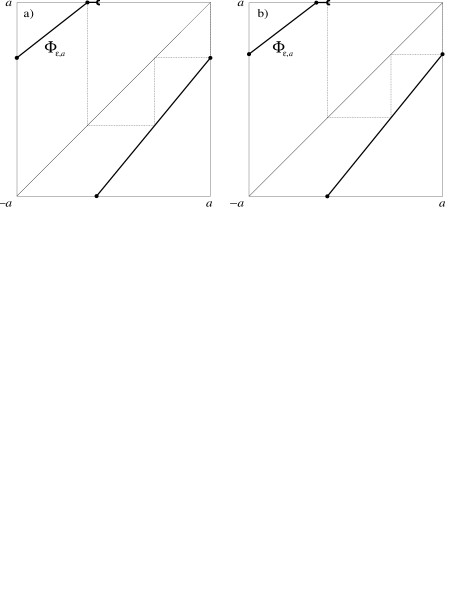
FIG. 1.: Moments of birth a) and death b) of the $v=1/3$ tongue for $a=0.5$. The $v=1/3$ tongue begins (ends) when the interfacial orbit, mapped through the auxiliary map $\Phi_{\varepsilon,a}$, collides with the left-most (right-most) extreme of the gap.

The auxiliary map is a map of the circle and it is possible to show [Carretero et al., 1997a] that the velocity of the travelling interface is given by its rotation number. The superstable region (the gap) of the auxiliary map induces a mode-locking of the rotation number as the parameters are varied. All the mode-locking regions, Arnold’s tongues, where any particular rational velocity $0\leq v(\varepsilon)=p/q\leq 1$ exists, may be computed analytically by finding the $(\varepsilon,a)$-interval for which the gap interval intersects the identity line after $q$ iterations passing $p$ times through the upper region of the auxiliary map. The extremes cases for this to happen arise from a border-collision bifurcation [Maistrenko et al., 1995] when an orbit starting in the gap falls at the beginning (end) of the gap interval after $q$ iterations. As an example we show in Fig. 1 the $v=1/3$ plateau limit orbits for $a=0.5$.

B Two-dimensional interface dynamics

When the gap size is non-negative the whole lattice was reduced to the one-dimensional auxiliary circle map. For negative gap size there are more than one site in the interface at the same time. Thus a one-dimensional reduction of the whole lattice does not seem attainable. However, thanks to the superstable basins $S_{\pm}$, the number of sites in the interface is still finite —less than or equal to $N$— and one could reduce the dynamics of the whole lattice to a $N$-dimensional system containing the information of the interface sites.

1 Minimal $N$-state layers

Before reducing the dynamics, one has to find the parameter regions where a particular number of sites is present in the interface. Define a minimal mass $N$-state or minimal $N$-state to be a minimal mass state having, during its evolution, a minimum of $N-1$ sites in the interface. The spatial discretization induces a change in the number of sites in the interface, so that the number of sites in the interface for a minimal $N$-state cannot be constant, it varies during its evolution between $N-1$ and $N$.

Suppose that the front shape at any time $t$ is given by $x_{t}(i)=h(i-vt)$, where $v$ is its travelling velocity and $h$ is a real valued function independent of $t$. The sites falling in the interface, are the sites contained in the interval $H=(h^{-1}(-a),h^{-1}(+a))$. Since the length of $H$ and the distance between nodes remains constant, the number of sites in $H$ can only vary by one during the evolution. In the case of a minimal $N$-state the number of sites in the interface is then $N$ or $N-1$. Nevertheless it is possible to remove this duality by a simple trick as it is shown in the next section. Using the same notation, the non-negative gap case corresponds to a minimal 1-state.

In order to show that a minimal $N$-state possesses $N$ or $N-1$ sites in the interface we supposed that the front shape is given by a function $h$. If the interfacial orbit is periodic it is easy to construct the front shape $h$ by considering any curve $h(i-vt)$ passing through all the points of the orbit. It is interesting to notice that such $h$ is not unique, in fact there exists an infinite number of possible $h$-functions passing through the finite collection of required points. On the other hand, when the velocity is irrational the interfacial orbit consists of an infinite number of distinct points. It is possible to reconstruct the front shape for irrational $v$ by superimposing snapshots of the front shape taken in a co-moving reference frame with velocity $v$. Extensive numerical experimentation suggests that the travelling interface is indeed given by an increasing function. Further reconstructions of travelling interfaces in more general types of CMLs are consistent with this result [Carretero et al., 1997c].

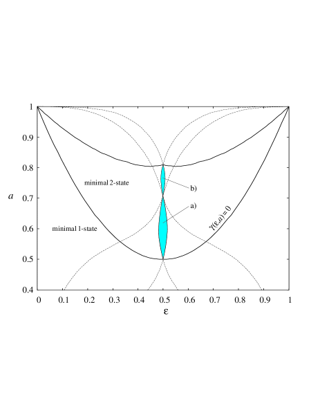
FIG. 2.: The $v=1/2$ tongues in the minimal 2-state layer. The tongues a) and b) are obtained by solving the inequalities (12) corresponding to the two possible period-2 orbits.

FIG. 3.: Tongues in the $N$-dimensional minimal $N$-state layers. The tongues for the velocities $v=1/2,\,2/5,\,1/3,\,2/7$ and $1/4$ (from right to left) in the minimal $N$-state layers for $N=1,\dots,8$ are presented.

In Fig. 2 we depict the $(\varepsilon,a)$ region where the minimal 2-state is present. The boundary between the minimal 1-state and the minimal 2-state layers is the zero-gap curve. Above that curve, the gap is negative, and there appears to be an infinite family of layers, labeled by $N$, and separated by boundary curves (cf. Fig. 3).

2 Two-dimensional auxiliary map

Throughout this section consider the case $N=2$, i.e. take $(\varepsilon,a)$-parameter values lying in the minimal 2-state layer. One would like to derive an auxiliary map that contains all the information of the interface dynamics as the auxiliary map $\Phi_{\varepsilon,a}$ does for the non-negative gap case. In order to find such map one has to take into account all possible evolution combinations of a minimal 2-state. The general form for a minimal 2-state $X_{t}$ is

$$X_{t}\,=\,(-1,\,x_{1},\,x_{2},\,1,\dots),$$

but because the size of the interface may be 1 or 2 one has the two possibilities $-a<x_{1}<x_{2}<a$ or $-a<x_{1}<a\leq x_{2}\leq 1$. Therefore, the first site, $x_{1}$, is always in the interface while the second, $x_{2}$, may or may not be in the interface. If the second site is not in the interface one could assign to it any value between $+a$ and $+1$ and its image by the piece-wise linear map $f_{a}$ would remain the same. In this case we choose to reduce $a\leq x_{2}\leq 1$ to $x_{2}=a$ and the dynamics is not altered. Using this reduction the site $x_{2}$ is now always included in the interface and it would be possible to remove the duality of having $2$ or $1$ sites in the minimal $2$-state layer.

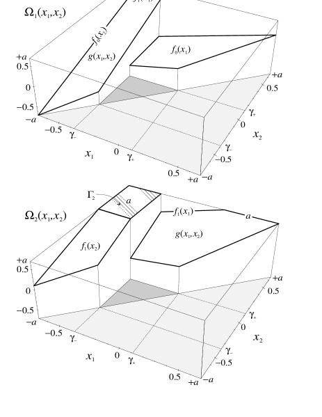
FIG. 4.: Example of the two-dimensional auxiliary map $\Omega(x_{1},x_{2})$$=$$\left(\Omega_{1}(x_{1},x_{2}),\Omega_{2}(x_{1},x_{2})\right)$ accounting for the interfacial sites dynamics in the minimal 2-state for $(\varepsilon,a)=(0.365,0.7)$.

It is possible to prove that the pair of interfacial sites $(x_{1},x_{2})$ is mapped to $(x^{\prime}_{1},x^{\prime}_{2})$ in 6 different ways depending on their value. The dynamics then induces a two-dimensional map $\Omega(x_{1},x_{2})=(x^{\prime}_{1},x^{\prime}_{2})$. An example of the map $\Omega$, obtained by considering all the possibilities is depicted in Fig. 4 by separating it into its two components $x^{\prime}_{1}=\Omega_{1}(x_{1},x_{2})$ and $x^{\prime}_{2}=\Omega_{2}(x_{1},x_{2})$. The shaded areas in Fig. 4 correspond to unreachable situations for a minimal 2-state. Since $X_{t}$ is a minimal mass state, $x_{2}$ has to be larger or equal to $x_{1}$, thus we eliminate the area where $x_{2}<x_{1}$ —light shaded area. On the other hand, it is straightforward to prove that if $x_{1}$ and $x_{2}$ are both at the same time in the interval $[\gamma_{-},\gamma_{+}]$, the succesive state is a minimal 3-state and thus we eliminate this possibility —dark shaded area. These forbidden areas are never reached by the dynamics.

For the 2-dimensional case (minimal 2-state layer) the auxiliary map $\Omega$ is a toral map in two dimensions —a toral map is the generalization of a circle map to more than one dimension (cf. [Baesens et al., 1991]). Generalizing the idea of rotation number in more dimensions one could think of a rotation vector [Baesens et al., 1991] whose entries correspond to the rotation number in every component. The rotation vector $\boldmath\rho$ $=(\rho_{1},\rho_{2})$ of $\Omega(x_{1},x_{2})$ is then two-dimensional. But since both sites $(x_{1},x_{2})$ belong to the same interface, that is moving with a defined velocity, the two components of the rotation vector have to be equal ($\rho_{1}=\rho_{2}$). In other words, the site $x_{1}$ has to travel at the same velocity than the site $x_{2}$ in order the interface to remain in the minimal 2-state layer. The only way $x_{1}$ would have different rotation number than $x_{2}$ is for an interface that is increasing (or decreasing) in size. Therefore instead of taking the whole rotation vector one may use a single scalar to describe the rotation around $\Omega(x_{1},x_{2})$. Thus, the velocity of the travelling interface in the minimal 2-state layer is given by this scalar, which will be simply called from now, the rotation number of $\Omega(x_{1},x_{2})$.

3 The tongues for the two-dimensional case

The two-dimensional auxiliary map $\Omega$ is piece-wise linear —it is a combination of planes— and possesses the analogue of the gap $\Gamma$ for the one-dimensional case: the region $[-a,\gamma_{-}]\times[\gamma_{+},a]$, see dashed plateau in Fig. 4. This region, which we refer to as the two-dimensional gap and denote by $\Gamma_{2}$, acts in the same way as its one-dimensional analogue. Any $(x_{1},x_{2})$-orbit falling into $\Gamma_{2}$ is superstable and therefore is parametrically stable to perturbations. This parametric stability gives rise to the mode-locking of the velocity. Thus one expects the minimal 2-state layer to contain Arnold’s tongues in the same way the minimal 1-state layer does.

Let us derive the tongues for $v=1/2$ in the two-dimensional case. First of all one has to choose the orbit. In the one-dimensional case the orbit was uniquely determined by a symbolic coding of the velocity for fixed values of $(\varepsilon,a)$ [Carretero et al., 1997a]. However, in the two-dimensional case, there are different possible evolutions for a given velocity. This is due to the fact that with more sites in the interface a wider selection of orbits is possible. The two orbits of a minimal 2-state giving a velocity $v=1/2$ correspond to a) $x_{2}\geq a$ all the times and b) alternating one and two sites in the interface. First of all the orbit has to be periodic (period two). Therefore we must have a) $f_{1}(x^{\prime}_{1}=f_{0}(x_{1}))=x_{1}$ and b) $g(x^{\prime}_{1}=f_{0}(x_{1}),x^{\prime}_{2}=f_{1}(x_{1}))=x_{1}$, i.e.,

$$\begin{array}[]{lccl}\hbox{a)}&x_{1}&=&{\displaystyle a(a(1-\varepsilon)-\varepsilon^{2})\over\displaystyle a^{2}-\varepsilon(1-\varepsilon)},\\[17.22217pt] \hbox{b)}&x_{1}&=&{\displaystyle a(1-2\varepsilon)\over\displaystyle a^{2}+2\varepsilon(\varepsilon-1)}.\end{array}$$ (11)

Next, one has to verify that the sites fall in the right intervals. That is

$$\begin{array}[]{lccl}\hbox{a)}&f_{1}(x_{1})>a\hbox{\quad and\quad}f_{0}(x^{\prime}_{1}=f_{0}(x_{1}))<-a,\\[8.61108pt] \hbox{b)}&f_{0}(x^{\prime}_{1}=f_{0}(x_{1}))<-a\hbox{\quad and\quad}f_{1}(x^{\prime}_{2}=f_{1}(x_{1}))>a.\end{array}$$ (12)

Combining Eqs. (11) and (12) gives the conditions that $\varepsilon$ and $a$ must satisfy in order to have the period-2 orbits. In Fig. 2 we display the regions where these conditions are satisfied in the minimal 2-state layer.

The same procedure may be applied to find the tongues for any rational velocity in the minimal 2-state layer. For every chosen $0<v=p/q<1$ there are $q$ possible different orbits, by combining 1 and 2 sites in the interface, and each one has a corresponding tongue in the minimal 2-state layer.

III $N$-Dimensional Interface Dynamics

Let us now consider the case of a minimal $N$-state layer for $N>2$. The dynamics in that layer may be reduced to a $N$-dimensional auxiliary toral map that controls the $N$-tuplet of sites in the interface. Again, thanks to the superstable region of the local map, this $N$-dimensional toral map will have a $N$-dimensional gap $\Gamma_{N}$ such that any $N$-tuplet in $\Gamma_{N}$ maps one of its components to $a$. The parametric stability is again induced by the presence of the gap $\Gamma_{N}$ when the latter exists.

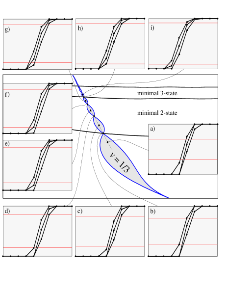
FIG. 5.: Successive states of the lattice in the $v=1/3$ tongue. Every time a site touches the boundary of the superstable region, in order to pass to a new configuration, the tongue $\varepsilon$-width is zero. The states from a) to i) correspond to increasing values of $a$ inside the $v=1/3$ tongues. The state a) is a minimal 1-state while the state b) is the transitional state to a minimal 2-state (zero gap). The states c), e) and g) correspond to the three different possibilities for a minimal 2-state and d) and f) correspond to the transition points between these three states. State i) is already is a minimal 3-state and h) is the transition point between the minimal 2-state to the minimal 3-state.

Thus, in every minimal $N$-state layer there are $q$ tongues corresponding to the velocity $v=p/q$ given by the $q$ possible combinations for the periodic-$q$ orbit of the $N$-dimensional auxiliary map. The regions where each tongue exists are given by a system of inequalities that the $N$-tuplet has to satisfy for the orbit to undergo the right combination of $N$ and $N-1$ sites in the interface. In Fig. 3 we show the tongues for the velocities $v=1/2,\,2/5,\,1/3,\,2/7$ and $1/4$, computed numerically, in the minimal $N$-state layers for $N=1,\dots,8$. We call the tongues in the minimal $N$-state layer the sub-$N$-tongues since they emanate from the principal mode-locking tongues, the principal tongues, for the one-dimensional case. Therefore, from every principal tongue there are $q$ corresponding sub-$N$-tongues in each $N$-layer. The structure of these sub-tongues is then self-similar and repeats itself in every layer as it may be observed in Fig. 3.

It is interesting to notice that because of the continuity of $v(\varepsilon,a)$ all the sub-$N$-tongues touch each other. Furthermore, the sub-$N$-tongues touch in a single point, i.e. in that particular point the width of the $\varepsilon$-mode-locked plateau (for a fixed value of $a$) is zero. This phenomenon repeats itself all along each family of sub-$N$-tongues and it happens every time a site of the interface touches the boundary of the superstable regions $S_{\pm}$ when varying the $(\varepsilon,a)$-parameters in order to go from one of the $q$ possible combinations of the interface orbit to the next. In Fig. 5 we show the state of the lattice at different stages of the $v=1/3$ tongue. The $\varepsilon$-width of the $v=1/3$ tongue is zero in the transitional case between two different interfacial orbits (cases b), d), f) and h)). One may consider this switch from one interfacial orbit to the next as a border-collision bifurcation of the attracting cycle of the-$N$-dimensional auxiliary map. In order to illustrate when this bifurcation takes place we show in Fig. 6 the bifurcation diagram of the attracting cycle of the interface in the $v=1/3$ tongue as the parameter $a$ is varied. From the figure it is possible to observe that when a stable point of the interface touches the boundary of the superstable region (thick dashed diagonal lines $a$ and $-a$) the attracting cycle changes because a further site is added to it. Where this happens (vertical dashed lines) the $\varepsilon$-width of the tongue is zero (see Fig. 5).

FIG. 6.: Bifurcation diagram of the attracting cycle of the interface sites in the $v=1/3$ tongue family. We plot the stable periodic 3 orbit of the interfacial sites as a function of the parameter $a$ after 10 000 transients. The values of $\varepsilon$ were taken such that the pair $(\varepsilon,a)$ remained in a path inside the $v=1/3$ mode-locked tongue (see dashed line inside the tongues in Fig. 5).

IV Generalizations

For every family of tongues for a particular mode-locked ratio there is an equivalent scenario as the one presented for $v=1/3$. The mode-locking regions could be computed analytically in every layer along with the attracting cycles and bifurcation diagrams. This is made possible by the simple form of the piece-wise linear local map. In more general CMLs, one way or diffusive, with bistable smooth local maps, the mode-locked regions still exist though they are not as large as in the piece-wise linear case because they typically involve an infinite number of sites in the interface [Carretero, 1997b]. The reduction of the dynamics to a toral map for the piece-wise linear local map requires a finite number of interfacial sites. Therefore it seems impossible to apply a toral map reduction of the dynamics for a generic CML. Nevertheless, if there exists an invariant travelling interface $h(i-vt)$ it is possible to reduce the dynamics of an infinite interface to a one-dimensional circle map whose rotation number describes the velocity of the travelling interface [Carretero et al., 1997c].

The border-collision bifurcations corresponding to transitions between families of sub-tongues prevails for more general CMLs and a similar scenario as the one depicted here for non-negative gap still exists. On the other hand, the border-collision bifurcations corresponding to transitions between sub-tongues of the same family, i.e. with the same rotation number, do not occur for smooth local maps. For the piece-wise linear CML these bifurcations came from a collision of a site with the border of the interface. For generic CMLs the interface is the whole interval $[x_{-}^{*},x_{+}^{*}]$ and thus it is impossible to have this kind of border-collision bifurcations.

REFERENCES

Baesens, C., Guckenheimer, J., Kim, S. & Mackay, R. S. [1991] “Three coupled oscillators: mode-locking, global bifurcations and toroidal chaos,” Physica D 49, 387–475.

Beck, C. [1994] “Chaotic cascade model for turbulent velocity distribution,” Phys. Rev. E 49(5), 3641–3652.

Carretero-González, R., Arrowsmith, D. K. & Vivaldi, F. [1997a] “Mode-locking in coupled map lattices”, Physica D 103, 381–403.

Carretero-González, R. [1997b] Front propagation and mode-locking in coupled map lattices. PhD thesis, Queen Mary and Westfield College, London, U.K.

Carretero-González, R., Arrowsmith, D. K. & Vivaldi, F. [1997c] “Reduction dynamics for travelling fronts in coupled map lattices,” in preparation.

Chaté, H. & Manneville, P. [1989] “Coupled map lattices as cellular automata,” J. Stat. Phys. 56(3/4), 357–370.

Chaté, H. & Manneville, P. [1990] “Using coupled map lattices to unveil structures in the space of cellular automata,” Springer proceedings in physics, Cellular automata and modeling of complex physical systems 46, 298–309.

Hassell, M. P., Miramontes, O., Rohani, P. & May, R. M. [1995] “Appropriate formulations for dispersal in spatially structured models,” Journal of Animal Ecology 64, 662–664.

Kaneko, K. [1983] “Transition from torus to chaos accompanied by frequency lockings with symmetry breaking,” Prog. Theor. Phys. 69(5), 1427.

Kaneko, K. [1984] “Period-doubling of kink-antikink patterns, quasiperiodicity in anti-ferro-like structures and spatial intermittency in coupled logistic lattice,” Prog. Theor. Phys. 72(3), 480–486.

Kaneko, K. [1985] “Spatial Period-doubling in open flow,” Phys. Lett. 111(7), 321–325.

Kaneko, K. [1986] “Turbulence in coupled map lattices,” Physica D 18, 475–476.

Kaneko, K. [1989] “Spatiotemporal chaos in one- and two-dimensional coupled map lattices,” Physica D 37, 60–82.

Kaneko, K. [1992] “Global travelling wave triggered by local phase slips,” Phys. Rev. Lett. 69(6), 905–908.

Kaneko, K. [1993] “Chaotic travelling waves in a coupled map lattice,” Physica D 68, 299–317.

Maistrenko, Y. L., Maistrenko, V. L., Vikul, S. I. & Chua, L. O. [1995] “Bifurcations of attracting cycles from the delayed Chua’s circuit,” Int. J. Bifurcation and Chaos 5(3), 653–671.

Solé, R. V. & Bascompte, J. [1995] “Measuring chaos from spatial information,” J. theo. Biol. 175, 139–147.

Willeboordse F. H. & Kaneko, K. [1995] “Pattern dynamics of a coupled map lattice for open flow,” Physica D 101–128.

Yanagita, T. & Kaneko, K. [1993] “Coupled map lattice model for convection,” Phys. Lett. A 175, 415–420.