On the accuracy of the semiclassical trace formula

Abstract

The semiclassical trace formula provides the basic construction from which one derives the semiclassical approximation for the spectrum of quantum systems which are chaotic in the classical limit. When the dimensionality of the system increases, the mean level spacing decreases as $\hbar^{d}$, while the semiclassical approximation is commonly believed to provide an accuracy of order $\hbar^{2}$, independently of $d$. If this were true, the semiclassical trace formula would be limited to systems in $d\leq 2$ only. In the present work we set about to define proper measures of the semiclassical spectral accuracy, and to propose theoretical and numerical evidence to the effect that the semiclassical accuracy, measured in units of the mean level spacing, depends only weakly (if at all) on the dimensionality. Detailed and thorough numerical tests were performed for the Sinai billiard in $2$ and $3$ dimensions, substantiating the theoretical arguments.

1 Introduction

The semiclassical analysis has proven to be a very useful tool in the field of “quantum chaos” as well as in many other fields. Nevertheless, one should bear in mind, that it only approximates the true quantal solution. Thus, it is imperative to know what are the errors which are inherent to the semiclassical approximation, and whether they could be considered as sufficiently small for the problem at hand.

We shall focus our attention on one particular application of the semiclassical approximation: The calculation of the energy spectra of classically chaotic systems. The analytical tool that is used for this purpose is the semiclassical Gutzwiller trace formula [1] which expresses the quantum spectral density in terms of classical quantities, and in particular the actions and stabilities of classical periodic orbits. The trace formula was used, among other things, to explain and discuss spectral statistics and their relation to the universal predictions of Random Matrix Theory (RMT) [2, 3]. However, a prerequisite for the use of the semiclassical approximation to compute short–range statistics is that it is able to reproduce the exact spectrum within an error which is comparable to or less than the mean level spacing! This is a demanding requirement, and quite often, the ability of the semiclassical approximation to reproduce precise levels for high–dimensional systems is doubted, and on the following grounds. The mean level spacing depends on the dimensionality (number of freedoms) of the system, and it is ${\cal O}(\hbar^{d})\cite[cite]{[\@@bibref{}{LLqm}{}{}]}$. Gutzwiller [1] uses an argument by Pauli [5] to show that in general the error margin for the semiclassical approximation scales as ${\cal O}(\hbar^{2})$ independently of the dimensionality. Applied to the trace formula, the expected error in units of the mean spacing, which is the figure of merit in the present context, is therefore expected to be ${\cal O}(\hbar^{2-d})$. We shall refer to this as the “traditional estimate”. It sets $d=2$ as a critical dimension for the applicability of the semiclassical trace formula and hence for the validity of the conclusions which are drawn from it. The few systems in $d>2$ dimensions which were numerically investigated display spectral statistics which adhere to the predictions of RMT as accurately as their counterparts in $d=2$ [6, 7, 8]. Thus, the “traditional estimate” cannot be entirely correct in the present context, and we shall explain the reasons why it is inadequate when we discuss other error bounds in the next section.

It is rather surprising that the problem of the accuracy of the semiclassical trace formula was rather rarely touched upon in the literature. Gutzwiller quotes the “traditional” estimate of ${\cal O}(\hbar^{2-d})$ which was discussed above [1, 9]. Gaspard and Alonso [10] and Alonso and Gaspard [11] derived explicit (generic) $\hbar$ corrections for the periodic orbit terms in the trace formula, but did not investigate their effect on the semiclassical accuracy of energy levels. Diffraction corrections were discussed in the context of the trace formula by Vattay, Wirzba and Rosenqvist [12] and by Primack et al. [13]. Also in these works the focus is on the corrections to individual periodic orbit terms rather than on the overall effect on energy levels. Boasman [14] studied the accuracy of the Boundary Integral Method (BIM) [15] for 2D billiards in the case that the exact kernel is replaced by its semiclassical asymptotic approximation. He finds that the resulting error is of the same magnitude as the mean spacing, which is consistent with the traditional estimate. However, Boasman’s work does not refer directly to the trace formula and to the periodic orbits contributions. The works of Bleher [16, 17] and of Prosen and Robnik [18] discuss the accuracy of the semiclassical approximation in the integrable case.

The purpose of this work is to address the subject of the accuracy of the semiclassical trace formula conceptually, theoretically and numerically. We shall be interested in particular in the dependence of the semiclassical error on the dimension of the system. To do so, we shall have to start by developing the basic concepts and define the measures we use for a quantitative estimate of the spectral error (section 2). The accuracy of the semiclassical approximation of the quantal energy spectrum will be then studied via the dual classical spectrum of actions and stabilities of periodic orbits (time spectrum). This will enable us to use our data base of quantum levels and periodic orbits for the Sinai billiards in two and three dimensions for a direct evaluation of the semiclassical error (section 3). We shall summarize the paper and discuss a few relevant points in section 4.

2 Measures of the semiclassical error

In order to define a proper error measure for the semiclassical approximation of the energy spectrum one has to clarify a few issues. In contrast with the EBK quantization which gives an explicit formula for the spectrum, the semiclassical spectrum for chaotic systems is implicit in the trace formula, or in the semiclassical expression for the spectral determinant. To extract the semiclassical spectrum we recall that the exact spectrum, $\{E_{n}\}$, can be obtained from the exact counting function:

$$N(E)\equiv\sum_{n=1}^{\infty}\Theta(E-E_{n})\ ,$$ (1)

by solving the equation

$$N(E_{n})=n-\frac{1}{2}\mskip 5.0mu plus 5.0mu,\mskip 5.0mu plus 5.0mu\mskip 5.0mu plus 5.0mun=1,2,\ldots\mskip 5.0mu plus 5.0mu\mskip 5.0mu plus 5.0mu\mskip 5.0mu plus 5.0mu.$$ (2)

In the last equation, an arbitrarily small amount of smoothing must be applied to the Heavyside function. In complete analogy, one obtains the semiclassical spectrum $\{E_{n}^{\rm sc}\}$ as [19]:

$$N_{\rm sc}(E_{n}^{\rm sc})=n-\frac{1}{2}\mskip 5.0mu plus 5.0mu,\mskip 5.0mu plus 5.0mu\mskip 5.0mu plus 5.0mun=1,2,\ldots\mskip 5.0mu plus 5.0mu\mskip 5.0mu plus 5.0mu\mskip 5.0mu plus 5.0mu,$$ (3)

where $N_{\rm sc}$ is a semiclassical approximation of $N$. Note that $N_{\rm sc}$ with which we start is not necessarily a sharp counting function. However, once $\{E_{n}^{\rm sc}\}$ is known, we can “rectify” the smooth $N_{\rm sc}$ into the sharp counting function $N^{\#}_{\rm sc}$ [3]:

$$N^{\#}_{\rm sc}(E)\equiv\sum_{n=1}^{\infty}\Theta(E-E_{n}^{\rm sc})\,.$$ (4)

The simplest choice for $N_{\rm sc}$ is the Gutzwiller trace formula [1] truncated at the Heisenberg time, which is what we shall use in the present paper. Alternatively, one can start from the regularized Berry–Keating Zeta function $\zeta_{\rm sc}(E)$ [20], and define $N_{\rm sc}=(1/\pi)\,\mbox{Im}\,\log\,\zeta_{\rm sc}(E+i0)$, in which case $N_{\rm sc}=N^{\#}_{\rm sc}$.

Next, in order to define a quantitative measure of the semiclassical error, one should establish a correspondence between the quantal and the semiclassical levels, namely, one should identify the semiclassical counterparts of the exact quantum levels. In classically chaotic systems, for which the Gutzwiller trace formula is applicable, the only constant of the motion is the energy. This is translated into a single “good” quantum number in the quantum spectrum, which is the ordinal number of the levels when ordered by their magnitude. Thus, the only correspondence which can be established between the exact spectrum $\{E_{n}\}$ and its semiclassical approximation, $\{E^{\rm sc}_{n}\}$, is

$$E_{n}\longleftrightarrow E^{\rm sc}_{n}\mskip 5.0mu plus 5.0mu.$$ (5)

This is to be contrasted with integrable systems, where it is appropriate to compare the exact and approximate levels which have the same quantum numbers.

The scale on which the accuracy of semiclassical energy levels should be measured depends, in general, on the problem at hand. The most natural choice, however, is the mean level spacing $(\bar{d}(E))^{-1}$ where $\bar{d}$ is the smooth density of states. The semiclassical error of the n’th level is therefore measured by [14]:

$$\epsilon_{n}\equiv\bar{d}(E_{n})\left(E_{n}-E^{\rm sc}_{n}\right).$$ (6)

A more useful and significant measure is the average of $\epsilon_{n}$ over an energy interval $\Delta E$ centered at $E$, which contains a large number of quantum energies, but which must be so small that both the classical dynamics and the mean density of states remain approximately constant. This energy averaging will be denoted by triangular brackets $\langle\cdot\rangle_{E}$ in the sequel. If the semiclassical mean density $\bar{d}_{\rm sc}$ agrees with $\bar{d}$ to a high precision, then obviously $\epsilon(E)\equiv\langle\epsilon_{n}\rangle_{E}=0$. In this case $\epsilon(E)$ is not a useful error measure. For billiard systems this is always the case, since the mean spectral density can be written as an asymptotic series with explicitly known coefficients [21, 22, 23]. For general systems, only the leading Weyl term is explicitly known. Two appropriate measures which are sensitive to the accuracy of the fluctuating parts of the level densities are the mean absolute error:

$$\epsilon^{\rm(1)}(E)\equiv\langle\ \bar{d}(E_{n})\left|E_{n}-E^{\rm sc}_{n}\right|\ \rangle_{E}$$ (7)

and the variance:

$$\epsilon^{\rm(2)}(E)\equiv\langle\ \left(\bar{d}(E_{n})\left(E_{n}-E^{\rm sc}_{n}\right)\right)^{2}\ \rangle_{E}\ .$$ (8)

Having defined the spectral error measures, let us apply them and try to get some estimates of the semiclassical error. In the introductory section we have mentioned the “traditional” estimate of the semiclassical error. Gutzwiller [1, 9] shows, based on Pauli [5], that the inherent error in the semiclassical (Van-Vleck) approximation of the quantal time propagator scales like ${\cal O}(\hbar^{2})$. Since the energy levels are the temporal Fourier components of the propagator, it is plausible to assume that they have the same degree of accuracy:

$$E_{n}-E^{\rm sc}_{n}={\cal O}(\hbar^{2})\mskip 5.0mu plus 5.0mu\mskip 5.0mu plus 5.0mu\mskip 5.0mu plus 5.0mu\mbox{``traditional''}.$$ (9)

(Strictly speaking, this is an upper bound.) The mean density of energy levels, for a general $d$-dimensional system is asymptotically given by Weyl’s formula [4]:

$$\bar{d}(E)\approx\frac{\omega(E)}{h^{d}}={\cal O}(\hbar^{-d})$$ (10)

where $\omega(E)$ is the measure of the energy surface in the classical phase space. Hence,

$$\epsilon^{\rm traditional}={\cal O}(\hbar^{2-d})\longrightarrow\left\{\begin{array}[]{lcc}{\rm const}&,&d=2\\ \infty&,&d\geq 3\end{array}\right.\mskip 5.0mu plus 5.0mu\mskip 5.0mu plus 5.0mu\mskip 5.0mu plus 5.0mu\mbox{as }\ \ \hbar\rightarrow 0.$$ (11)

That is, the semiclassical approximation is (marginally) accurate in 2 dimensions, but it fails to predict accurate energy levels for 3 dimensions or more.

One may get a different estimate of the semiclassical error, if the Gutzwiller Trace Formula (GTF) is used as a starting point. Suppose that we have calculated $N_{\rm sc}$ to a certain degree of precision, and we compute from it the semiclassical energies using (3). The quality of this approximation can be estimated if the leading corrections $\Delta N_{\rm sc}$ are also included and the resulting energy differences $\delta_{n}$ are evaluated. We thus need to consider:

$$N_{\rm sc}(E_{n}^{\rm sc}+\delta_{n})+\Delta N_{\rm sc}(E_{n}^{\rm sc}+\delta_{n})=n-\frac{1}{2}\,.$$ (12)

Combining (3) and (12) we get to first order in $\delta_{n}$:

$$\delta_{n}\approx\frac{\Delta N_{\rm sc}(E_{n}^{\rm sc})}{\partial N_{\rm sc}(E_{n}^{\rm sc})/\partial E}\approx\frac{\Delta N_{\rm sc}(E_{n}^{\rm sc})}{\bar{d}(E_{n}^{\rm sc})}.$$ (13)

In the above we assumed that the fluctuations of $N_{\rm sc}$ around its average are not very large. Thus,

$$\epsilon^{\rm GTF}\approx\bar{d}(E_{n}^{\rm sc})\delta_{n}\approx\Delta N_{\rm sc}(E_{n}^{\rm sc}).$$ (14)

Let us apply the above formula and consider the case in which we take for $N_{\rm sc}$ its mean part $\bf\bar{\it N}$, and that we include in $\bf\bar{\it N}$ terms of order up to (and including) $\hbar^{-m},m\leq d$. For $\Delta N_{\rm sc}$ we use both the leading correction to $\bf\bar{\it N}$ and the leading order periodic orbit sum which is (formally) of order $\hbar^{0}$. Hence,

$$\epsilon^{\rm GTF}_{\bar{N}}={\cal O}(\hbar^{-m+1})+{\cal O}(\hbar^{0})={\cal O}\left(\hbar^{\min(-m+1,\,0)}\right).$$ (15)

We conclude, that approximating the energies only by the mean counting function $\bf\bar{\it N}$ up to (and not including) the constant term, is already sufficient to obtain semiclassical energies which are accurate to ${\cal O}(\hbar^{0})={\cal O}(1)$ with respect to the mean density of states. Note again, that no periodic orbits were included in $N_{\rm sc}$. Including less terms in $\bf\bar{\it N}$ will lead to a diverging semiclassical error, while more terms will be masked by the periodic orbit (oscillatory) term. One can do even better if one includes in $N_{\rm sc}$ the smooth terms up to and including the constant term (${\cal O}(\hbar^{0})$) together with the leading order periodic orbit sum which is formally also ${\cal O}(\hbar^{0})$. The semiclassical error is then:

$$\epsilon^{\rm GTF}_{\rm po}={\cal O}(\hbar^{1}).$$ (16)

That is, the semiclassical energies measured in units of the mean level spacing are asymptotically accurate independently of the dimension! This estimate grossly contradicts the “traditional” estimate (11) and calls for an explanation.

The first point that should be noted is that the order of magnitude (power of $\hbar$) of the periodic orbit sum, which we considered above to be ${\cal O}(\hbar^{0})$, is only a formal one. Indeed, each term which is due to a single periodic orbit is of order ${\cal O}(\hbar^{0})$. However the periodic orbit sum absolutely diverges, and at best it is only conditionally convergent. To give it a numerical meaning, the periodic orbit sum must therefore be regularized. This is effectively achieved by truncating the trace formula or the corresponding spectral $\zeta$ function [24, 25, 20, 26]. However, the truncation cutoff itself depends on $\hbar$. One can conclude, that the simple minded estimate (16) given above is at best a lower bound, and the error introduced by the periodic orbit sum must be re-evaluated with more care. This point will be dealt with in great detail in the sequel, and we shall eventually develop a meaningful framework for evaluating the magnitude of the periodic orbit sum.

The connection and the disparity between the “traditional” estimate of the semiclassical error and the one based on the trace formula can be further illustrated by the following argument. The periodic orbit formula is derived from the semiclassical propagator $K_{\rm sc}$ using further approximations [1]. One thus wonders, how can it be that further approximations of $K_{\rm sc}$ actually reduce the semiclassical error from (11) to (16)? The puzzle is resolved if we recall, that in order to obtain $\epsilon^{\rm GTF}_{\rm po}$ above we separated the density of states into a smooth and an oscillating parts, and we required that the smooth part is accurate enough. To achieve this, we have to go beyond the leading Weyl’s term and to use specialized methods to calculate the smooth density of states beyond the leading order. These methods are mostly developed for billiards [21, 22, 23]. In any case, to obtain $\epsilon^{\rm GTF}_{\rm po}$ we have added an additional information which goes beyond the leading semiclassical approximation.

A straightforward check of the accuracy of the semiclassical spectrum using the error measures $\epsilon,\epsilon^{\rm(1)},\epsilon^{\rm(2)}$ is exceedingly difficult due to the large number of periodic orbits needed because of the exponential proliferation in chaotic systems. The few cases where such tests were carried out involve 2D systems and it was possible to check only the lowest (less than a hundred) levels (e.g. [27, 28]). The good agreement between the exact and the semiclassical values confirmed the expectation that in 2D the semiclassical error is small. In 3D, the topological entropy is typically much larger [19, 7], and the direct test of the semiclassical spectrum becomes prohibitive.

Facing with this grim reality, we have to introduce alternative error measures which yield the desired information, but which are more appropriate for a practical calculation. We construct the measure:

$$\delta^{\rm(2)}(E)\equiv\left\langle\left|N(E)-N_{\rm sc}^{\#}(E)\right|^{2}\right\rangle_{E}\ .$$ (17)

As before, the triangular brackets indicate averaging over an energy interval $\Delta E$ about $E$. We shall now show that $\delta^{\rm(2)}$ faithfully reflects the deviations between the spectra, and is closely related to $\epsilon^{\rm(1)}$ and $\epsilon^{\rm(2)}$. Note, that the following arguments are purely statistical and apply to every pair of staircase functions.

Suppose first, that all the differences $E_{n}^{\rm sc}-E_{n}$ are smaller than the mean spacing. Then, $|N-N_{\rm sc}^{\#}|$ is either 0 or 1 (see figure 1) and hence $|N-N_{\rm sc}^{\#}|=|N-N_{\rm sc}^{\#}|^{2}$. Consequently,

$$\delta^{\rm(2)}(E)\approx\left\langle\left|N(E)-N_{\rm sc}^{\#}(E)\right|\right\rangle_{E}\mskip 5.0mu plus 5.0mu,\mskip 5.0mu plus 5.0mu\mskip 5.0mu plus 5.0mu\mskip 5.0mu plus 5.0mu\mbox{small deviations}\,.$$ (18)

However, the right hand side of the above equation (the fraction of non–zero contributions) equals $\epsilon^{\rm(1)}$. Thus,

$$\delta^{\rm(2)}\approx\epsilon^{\rm(1)}\mskip 5.0mu plus 5.0mu,\mskip 5.0mu plus 5.0mu\mskip 5.0mu plus 5.0mu\mskip 5.0mu plus 5.0mu\mbox{small deviations}\ .$$ (19)

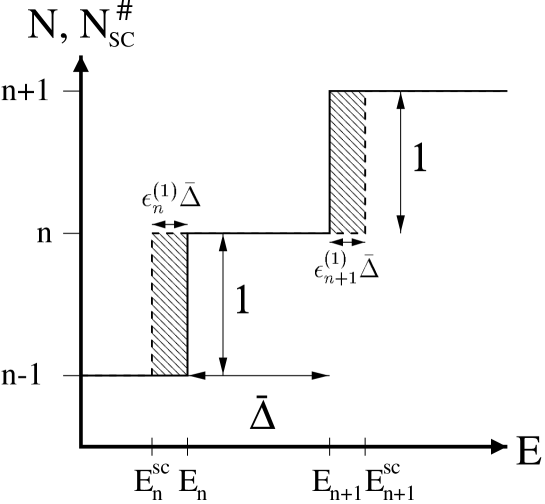
Figure 1: Illustration of $|N(E)-N_{\rm sc}^{\#}(E)|$ for small deviations between quantum and semiclassical energies: $\epsilon^{\rm(1)}\ll\bar{d}^{-1}\equiv\bar{\Delta}$. The quantum staircase $N(E)$ is denoted by the full line and the semiclassical staircase $N_{\rm sc}^{\#}(E)$ is denoted by the dashed line. The difference is shaded.

If, on the other hand, deviations are much larger than one mean spacing, the typical horizontal distance $\bar{d}|E-E_{n}|$ should be comparable to the vertical distance $|N-N_{\rm sc}^{\#}|$, and hence, in this limit

$$\delta^{\rm(2)}\approx\epsilon^{\rm(2)}\mskip 5.0mu plus 5.0mu,\mskip 5.0mu plus 5.0mu\mskip 5.0mu plus 5.0mu\mskip 5.0mu plus 5.0mu\mbox{large deviations}\,.$$ (20)

Therefore, we expect $\delta^{\rm(2)}$ to interpolate between $\epsilon^{\rm(1)}$ and $\epsilon^{\rm(2)}$ throughout the entire range of deviations. This behavior is indeed observed in a numerical test which was performed to check the above expectations. We considered the unfolded exact spectrum (normalized to unity mean spacing [29]) of the 3D Sinai billiard $\{X_{n}\}$ and created from it a synthetic spectrum by adding a random variable with $0$ mean and variance $\sigma^{2}$:

$$X^{\sigma}_{n}=X_{n}+X_{\rm random}(0,\sigma).$$ (21)

The $\{X^{\sigma}_{n}\}$ has also a unity mean spacing and it is meant to imitate a semiclassical spectrum. After sorting $\{X^{\sigma}_{n}\}$ we calculated the measures $\epsilon^{\rm(1)},\epsilon^{\rm(2)}$ and $\delta^{\rm(2)}$ as functions of $\sigma$. The results are shown in figure 2, and they verify the estimates (19, 20) in the appropriate limits.

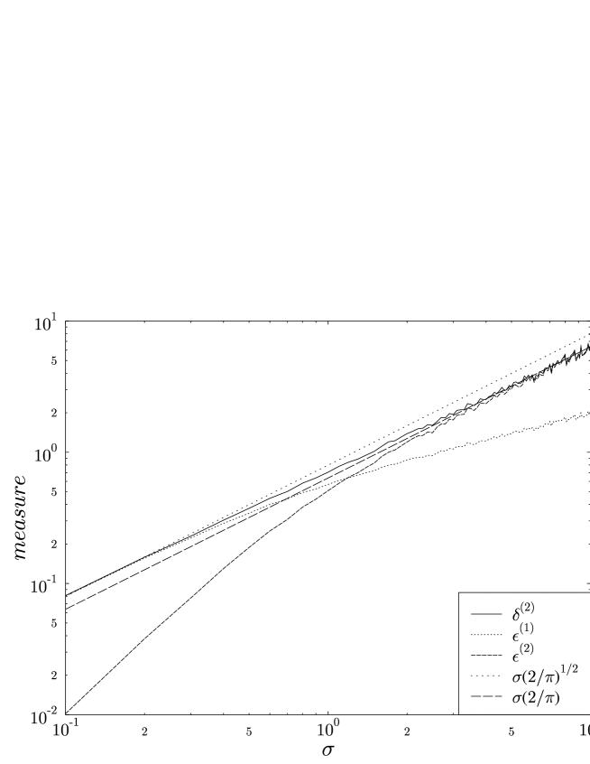
Figure 2: The spectral measures $\epsilon^{\rm(1)},\epsilon^{\rm(2)},\delta^{\rm(2)}$ and and their asymptotics for a wide range of spectral deviations $\sigma$. The random distribution was Gaussian, and similar results were obtained also for a uniform distribution. Note the logarithmic scale.

The numerical test reported in figure 3 demonstrates another attractive feature of the measure $\delta^{\rm(2)}$: It is completely equivalent to $\epsilon^{\rm(2)}$ when the spectral counting functions are replaced by their smooth counterparts, provided that the smoothing width is of the order of 1 mean level spacing and the same smoothing is applied to both counting functions. That is,

$$\delta^{\rm(2)}_{\rm smooth}\approx\epsilon^{\rm(2)}$$ (22)

for all deviations. (In fact, for small deviations there is a proportionality factor, but it can be set to 1 if an appropriate smoothing is used.) In testing the semiclassical accuracy, this kind of smoothing is essential and will be introduced by truncating the trace formula at the Heisenberg time $t_{\rm H}\equiv h\bar{d}$.

Figure 3: Comparison of the measures $\delta^{\rm(2)}_{\rm smooth}$ and $\epsilon^{\rm(2)}$ for a wide range of spectral deviations $\sigma$ and for Gaussian distribution. The difference is also plotted since the curves almost overlap. Note the logarithmic scale.

These properties of the measure $\delta^{\rm(2)}$, and its complete equivalence to $\epsilon^{\rm(2)}$ for smooth counting functions, renders it a most appropriate measure of the semiclassical error.

We now turn to the practical evaluation of $\delta^{\rm(2)}$. To affect the energy averaging, we choose a positive window function $w(E^{\prime}-E)$ which has a width $\Delta E$ near $E$ and is normalized by $\int_{-\infty}^{+\infty}{\rm d}E^{\prime}w^{2}(E^{\prime})=1$. It falls off sufficiently rapidly so that all the expressions which follow are well behaved. Construct the following counting functions that have an effective support on an interval of size $\Delta E$ about $E$:

$$\hat{N}(E^{\prime};E) \equiv w(E^{\prime}{-}E)N(E^{\prime})$$ (23)

$$\hat{N}_{\rm sc}^{\#}(E^{\prime};E) \equiv w(E^{\prime}{-}E)N_{\rm sc}^{\#}(E^{\prime})\,.$$ (24)

At this stage $\hat{N}$ and $\hat{N}_{\rm sc}^{\#}$ are still sharp staircases, and we note that the multiplication with $w$ preserves the sharpness of the stairs (it is not a convolution!). We now explicitly construct $\delta^{\rm(2)}(E)$ as:

$$\delta^{\rm(2)}(E) = \int_{-\infty}^{+\infty}{\rm d}E^{\prime}\,\left|\hat{N}(E^{\prime};E)-\hat{N}_{\rm sc}^{\#}(E^{\prime};E)\right|^{2}$$ (25)

$$= \int_{-\infty}^{+\infty}{\rm d}E^{\prime}\,\left|N(E^{\prime})-N_{\rm sc}^{\#}(E^{\prime})\right|^{2}w^{2}(E^{\prime}-E).$$

To construct $\delta^{\rm(2)}_{\rm smooth}$ we need to smooth $N,N_{\rm sc}^{\#}$ over a scale of order of one mean spacing. This can be done e.g. by replacing the sharp stairs by error functions. As for $N_{\rm sc}^{\#}$, we prefer to simply replace it with the original $N_{\rm sc}$, which we assume to be smooth over one mean spacing. That is, we suppose that $N_{\rm sc}$ contains periodic orbits up to Heisenberg time. Hence,

$$\delta^{\rm(2)}_{\rm smooth}(E)=\int_{-\infty}^{+\infty}{\rm d}E^{\prime}\,\left|N^{\rm smooth}(E^{\prime})-N_{\rm sc}(E^{\prime})\right|^{2}w^{2}(E^{\prime}-E).$$ (26)

A comment is in order here. Strictly speaking, to satisfy (22) we need to apply the same smoothing to $N$ and to $N_{\rm sc}^{\#}$, and in general $N_{\rm sc}^{\#,{\rm smooth}}\neq N_{\rm sc}$, but there are differences of order 1 between the two functions. However, since our goal is to determine whether the semiclassical error remains finite or diverges in the semiclassical limit $\hbar\rightarrow 0$, we disregard such inaccuracies of order 1. If more accurate error measure is needed, then more care should be practiced in this and in the following steps.

Applying Parseval’s theorem to (26) we get:

$$\delta^{\rm(2)}_{\rm smooth}(E)=\frac{1}{\hbar}\int_{-\infty}^{+\infty}{\rm d}t\,\left|\hat{D}(t;E)-\hat{D}_{\rm sc}(t;E)\right|^{2}$$ (27)

where

$$\hat{D}(t;E) \equiv \frac{1}{\sqrt{2\pi}}\int_{-\infty}^{+\infty}{\rm d}E^{\prime}\,\hat{N}^{\rm smooth}(E^{\prime};E)\exp(iE^{\prime}t/\hbar)$$ (28)

$$\hat{D}_{\rm sc}(t;E) \equiv \frac{1}{\sqrt{2\pi}}\int_{-\infty}^{+\infty}{\rm d}E^{\prime}\,\hat{N}_{\rm sc}(E^{\prime};E)\exp(iE^{\prime}t/\hbar).$$ (29)

We shall refer to $\hat{D},\hat{D}_{\rm sc}$ as the (regularized) quantal and semiclassical time spectra, respectively. This name can be justified by invoking the Gutzwiller trace formula and expressing the semiclassical counting function as a mean part plus a sum over periodic orbits. We have:

$$N_{\rm sc}(E)=\bar{N}(E)+\sum_{\rm po}\frac{\hbar A_{j}(E)}{T_{j}(E)}\sin[S_{j}(E)/\hbar-\nu_{j}\pi/2]\ ,$$ (30)

where $A_{j}=T_{j}/(\pi\hbar r_{j}\sqrt{|I-M_{j}|})$ is the semiclassical amplitude of the j’th periodic orbit, and $T_{j},S_{j},\nu_{j},M_{j},r_{j}$ are its period, action, Maslov index, monodromy and repetition index, respectively. Then, the corresponding time spectrum reads:

$$\hat{D}_{\rm sc}(t;E) \approx \bar{D}(t;E)$$

$$+ \frac{1}{2i}\sum_{\rm po}\frac{\hbar A_{j}(E)}{T_{j}(E)}\left\{{\rm e}^{(i/\hbar)[Et+S_{j}(E)]}\hat{w}([t+T_{j}(E)]/\hbar)-\right.$$

$$\left.\mskip 5.0mu plus 5.0mu\mskip 5.0mu plus 5.0mu\mskip 5.0mu plus 5.0mu\mskip 5.0mu plus 5.0mu\mskip 5.0mu plus 5.0mu\mskip 5.0mu plus 5.0mu\mskip 5.0mu plus 5.0mu\mskip 5.0mu plus 5.0mu\mskip 5.0mu plus 5.0mu\mskip 5.0mu plus 5.0mu\mskip 5.0mu plus 5.0mu\mskip 5.0mu plus 5.0mu\mskip 5.0mu plus 5.0mu\mskip 5.0mu plus 5.0mu\mskip 5.0mu plus 5.0mu\mskip 5.0mu plus 5.0mu\mskip 5.0mu plus 5.0mu\mskip 5.0mu plus 5.0mu\mskip 5.0mu plus 5.0mu\mskip 5.0mu plus 5.0mu\mskip 5.0mu plus 5.0mu\mskip 5.0mu plus 5.0mu\mskip 5.0mu plus 5.0mu{\rm e}^{(i/\hbar)[Et-S_{j}(E)]}\hat{w}([t-T_{j}(E)]/\hbar)\right\}.$$

In the above, the Fourier transform of $w$ is denoted by $\hat{w}$. It is a localized function of $t$ whose width is $\Delta t\approx\hbar/\Delta E$. The sum over the periodic orbits in $D_{\rm sc}$ therefore produces sharp peaks centered at times that correspond to the periods $T_{j}$, hence the name “time spectrum”. The term $\bar{D}$ corresponds to the smooth part and thus is sharply peaked near $t=0$. To obtain (2) we expanded the actions near $E$ to first order: $S_{j}(E^{\prime})\approx S_{j}(E)+(E^{\prime}-E)T_{j}(E)$. We note in passing, that this approximate expansion of $S_{j}$ can be avoided altogether if one performs the Fourier transform over $\hbar^{-1}$ rather than over the energy. This way, an action spectrum will emerge, but also here the action resolution will be finite, because the range of $\hbar^{-1}$ should be limited to the range where $\bar{d}(E;\hbar)$ is approximately constant. It turns out therefore, that the two approaches are essentially equivalent, and for billiards they are identical.

The manipulations done thus far were purely formal, and did not manifestly circumvent the difficult task of evaluating $\delta^{\rm(2)}_{\rm smooth}$. However, the introduction of the time spectra and the formula (27) put us in a better position than with the original expression (25). The advantages of using the time spectra in the present context are the following:

• The semiclassical time spectrum $\hat{D}_{\rm sc}(t;E)$ is absolutely convergent for all times (as long as the window function $w$ is well behaved, e.g. it is a Gaussian). This statement is correct even if the sum (2) extends over the entire set of periodic orbits! This is in contrast with the trace formula expression for $N_{\rm sc}$ (and therefore $\hat{N}_{\rm sc}$) which is absolutely divergent if all of the periodic orbits are included.

• Time scale separation: As we noted above, the time spectrum is peaked at times that correspond to periods of the classical periodic orbits. This allows us to distinguish between various qualitatively different types of contributions to $\delta^{\rm(2)}_{\rm smooth}$.

We shall now pursue the separation of the time scales in detail. We first note, that due to $\hat{N},\hat{N}_{\rm sc}$ being real, there is a $t\leftrightarrow(-t)$ symmetry in (27) and therefore $\delta^{\rm(2)}=2\int_{0}^{\infty}\cdots$. We now divide the time axis into four intervals :

  

$\bf 0\leq t\leq\Delta t$: The shortest time scale in our problem is $\Delta t=\hbar/\Delta E$. The contributions to this time interval are due to the differences between the exact and the semiclassical mean densities of states. This is an important observation, since it allows us to distinguish between the two sources of semiclassical error — the error that emerges from the mean densities and the error that originates from the fluctuating part (periodic orbits). Since we are interested only in the semiclassical error that results from the fluctuating part of the spectral density, we shall ignore this regime in the following.

  $\bf\Delta t\leq t\leq t_{\rm erg}$

: This is the non–universal regime [29], in which periodic orbits are still sparse, and cannot be characterized statistically in a significant fashion. The “ergodic” time scale $t_{\rm erg}$ is purely classical and is independent of $\hbar$.

  

$\bf t_{\rm erg}\leq t\leq t_{\rm H}$: In this time regime periodic orbits are already in the universal regime and are dense enough to justify a statistical approach to their proliferation and stability. The upper limit of this interval is the Heisenberg time $t_{\rm H}=h\bar{d}(E)$, which is the time that is needed to resolve the quantum (discrete) nature of a wavepacket with energy concentrated near $E$. The Heisenberg time is “quantum” in the sense that it is dependent of $\hbar$: $t_{\rm H}={\cal O}(\hbar^{1-d})$.

  

$\bf t_{\rm H}\leq t<\infty$: This is the interval of “long” orbits which is effectively truncated from the integration as a result of introducing a smoothing of the quantal and semiclassical counting functions, with a smoothing scale of the order of a mean level spacing.

Dividing the integral (27) according to the above time intervals, we can rewrite $\delta^{\rm(2)}_{\rm smooth}$:

$$\delta^{\rm(2)}_{\rm smooth}(E) = \left(\int_{\Delta t}^{t_{\rm erg}}+\int_{t_{\rm erg}}^{t_{\rm H}}+\int_{t_{\rm H}}^{\infty}\right)\frac{2{\rm d}t}{\hbar}\,\left|\hat{D}(t;E)-\hat{D}_{\rm sc}(t;E)\right|^{2}$$ (32)

$$\equiv \delta^{\rm(2)}_{\rm short}+\delta^{\rm(2)}_{\rm m}+\delta^{\rm(2)}_{\rm long}\mskip 5.0mu plus 5.0mu.$$

As explained above, $\delta^{\rm(2)}_{\rm long}$ can be ignored due to smoothing on the scale of a mean level spacing. The integral $\delta^{\rm(2)}_{\rm short}$ is to be neglected for the following reason. The integral extends over a time interval which is finite and independent of $\hbar$, and therefore it contains a fixed number of periodic orbits contributions. The semiclassical approximation provides, for each individual contribution, the leading order in $\hbar$, and therefore [30] we should expect:

$$\delta^{\rm(2)}_{\rm short}\longrightarrow 0\mskip 5.0mu plus 5.0mu\mskip 5.0mu plus 5.0mu\mskip 5.0mu plus 5.0mu\mbox{as }\mskip 5.0mu plus 5.0mu\hbar\longrightarrow 0.$$ (33)

The purpose of this work is to check whether the semiclassical error is finite or divergent as $\hbar\longrightarrow 0$, and to study if the rate of divergence depends on dimensionality. Equation (33) implies that $\delta^{\rm(2)}_{\rm short}$ cannot affect $\delta^{\rm(2)}$ in the semiclassical limit and we shall neglect it in the following.

We thus remain with a lower bound for our measure:

$$\delta^{\rm(2)}_{\rm smooth}\approx\delta^{\rm(2)}_{\rm m}$$ (34)

which is going to be our object of interest from now on.

The fact that $t_{\rm H}$ is extremely large on the classical scale renders the calculation of all the periodic orbits with periods less than $t_{\rm H}$ an impossible task. However, sums over periodic orbits when the period is longer than $t_{\rm erg}$ tend to meaningful limits, and hence, we would like to recast the expression for $\delta^{\rm(2)}_{\rm m}$ in the following way. Write $\delta^{\rm(2)}_{\rm m}$ as:

$$\delta^{\rm(2)}_{\rm m} = \frac{2}{\hbar}\int_{t_{\rm erg}}^{t_{\rm H}}{\rm d}t\,\left\langle\left|\hat{D}(t)-\hat{D}_{\rm sc}(t)\right|^{2}\right\rangle_{t}$$ (35)

$$= \frac{2}{\hbar}\int_{t_{\rm erg}}^{t_{\rm H}}{\rm d}t\,\left\langle\left|\hat{D}(t)\right|^{2}\right\rangle_{t}\times\left[\frac{\left\langle\left|\hat{D}(t)-\hat{D}_{\rm sc}(t)\right|^{2}\right\rangle_{t}}{\left\langle\left|\hat{D}(t)\right|^{2}\right\rangle_{t}}\right]$$ (36)

$$\equiv \frac{2}{\hbar}\int_{t_{\rm erg}}^{t_{\rm H}}{\rm d}t\,\left\langle\left|\hat{D}(t)\right|^{2}\right\rangle_{t}\times C(t)$$

$$= \int_{t_{\rm erg}}^{t_{\rm H}}\mbox{envelope}\times\mbox{correlation}\,$$

where the parametric dependence on $E$ was omitted for brevity. The smoothing over $t$ is explicitly indicated to emphasize that one may use a statistical interpretation of the terms of the integrand. This is so because in this domain, the density of periodic orbits is so large, that within a time interval of width $\hbar/\Delta E$ there are exponentially many orbits whose contributions are averaged due to the finite resolution.

We note now that we can use the following relation between the time spectrum and the spectral form factor $K(\tau)$:

$$\frac{\left\langle\left|\hat{D}(t)\right|^{2}\right\rangle_{t}}{\hbar}\,{\rm d}t=\frac{K(\tau)}{4\pi^{2}\tau^{2}}\,{\rm d}\tau$$ (38)

where $\tau\equiv t/t_{\rm H}$ is the scaled time. The above form factor is smoothed according to the window function  $w$. Hence:

$$\delta^{\rm(2)}_{\rm smooth}\approx\frac{1}{2\pi^{2}}\int_{\tau_{\rm erg}}^{1}{\rm d}\tau\,\frac{K(\tau)C(\tau)}{\tau^{2}}\,.$$ (39)

For generic chaotic systems we expect that $K(\tau)$ agrees with the results of RMT in the universal regime $\tau>\tau_{\rm erg}$ [31, 2, 29], and therefore

$$K(\tau)\approx g\tau\mskip 5.0mu plus 5.0mu\mskip 5.0mu plus 5.0mu\mskip 5.0mu plus 5.0mu\mbox{for }\tau_{\rm erg}<\tau\leq 1,$$ (40)

where $g=1$ for systems which violate time reversal symmetry, and $g=2$ if time reversal symmetry is respected. This implies that the evaluation of $\delta^{\rm(2)}_{\rm smooth}$ reduces to

$$\delta^{\rm(2)}_{\rm smooth}\approx\frac{g}{2\pi^{2}}\int_{\tau_{\rm erg}}^{1}{\rm d}\tau\,\frac{C(\tau)}{\tau}.$$ (41)

The dependence on $\hbar$ in this expression comes from the lower integration limit which is proportional to $\hbar^{d-1}$ as well as from the implicit dependence of the function $C$ on $\hbar$.

Formula (41) is our main theoretical result. However, we do not know how to evaluate the correlation function $C(\tau)$ from first principles. The knowledge of the $\hbar$ corrections to each of the terms in the semiclassical time spectrum is not sufficient since the resulting series which ought to be summed is not absolutely convergent (see detailed discussion in section (4)). Therefore we have to recourse to a numerical analysis, which will be described in the next section. The numerical approach requires one further approximation, which is imposed by the fact that the number of periodic orbits with $t<t_{\rm H}$ is prohibitively large. We had to limit the data base of periodic orbit to the domain $t<t_{\rm cpu}$ with $t_{\rm erg}\ll t_{\rm cpu}\ll t_{\rm H}$. The time $t_{\rm cpu}$ has no physical origin, and it represents only the limits of our computational resources. Using the available numerical data we were able to compute $C(t)$ numerically for all $t_{\rm erg}<t<t_{\rm cpu}$ and we then extrapolated it to the entire domain of interest. We consider this extrapolation procedure to be the main source of uncertainty. However, since the extrapolation is carried out in the universal regime, it should be valid if there are no other time scales between $t_{\rm erg}$ and $t_{\rm H}$.

3 Numerical results

We used the formalism and definitions presented above to check the accuracy of the semiclassical spectra of the 2D and 3D Sinai billiards. The most important ingredient in this numerical study is that we could apply the same analysis to the two systems, and by comparing them to give a reliable answer to the main question posed in this work, namely, how does the semiclassical accuracy depend on dimensionality.

The classical dynamics in billiards depends trivially on the energy (velocity), and therefore the relevant parameter is the length rather than the period of the periodic orbits. Because of the same reason, the quantum wavenumbers $k_{n}\equiv\sqrt{2mE_{n}}/\hbar$ are the relevant variables in the quantum description. From now on we shall use the variables $(l,k)$ instead of $(t,E)$, and use “length spectra” rather than “time spectra”. The semiclassical limit is obtained for $k\rightarrow\infty$ and ${\cal O}(\hbar)$ is equivalent to ${\cal O}(k^{-1})$. Note also that for a billiard $\bar{N}(k)\approx Ak^{d}$ where $A$ is a proportional to the billiard’s volume.

The numerical work is based on the quantum spectra and on the classical periodic orbits which were calculated by Schanz and Smilansky [32, 33] for the 2D billiard, and by Primack and Smilansky [6, 7] for the 3D billiard. The numerical methods and the checks performed to ensure that the quantum and the classical data bases are accurate, complete and immaculate are discussed in the papers cited above.

We start with the 2D Sinai billiard, which is the free space between a square of edge $L$ and an inscribed disc of radius $R$, with $2R<L$. In our case we used $L=1$ and $R=0.25$ and considered the quarter desymmetrized billiard (see figure 4) with Dirichlet boundary conditions for the quantum calculations. The quantal data base consisted of the lowest 27645 eigenvalues in the range $0<k<1320$, with eigenstates which are either symmetric or antisymmetric with respect to reflection on the main diagonal. The classical data base consisted of the shortest 20273 periodic orbits (including time reversal, reflection symmetries and repetitions) in the length range $0<l<5$. For each orbit, the length, the stability determinant and the reflection phase were recorded.

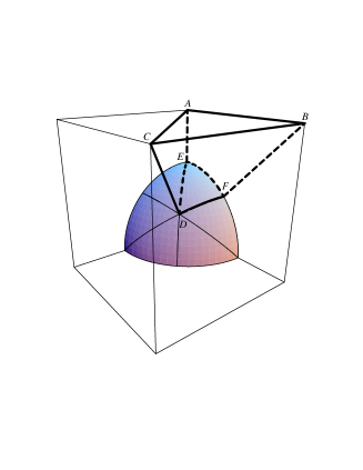
Figure 4: Left: The quarter desymmetrized 2D Sinai billiard. Right: The fully ($1/48$) desymmetrized 3D Sinai billiard (bold lines).

We begin the numerical analysis of the 2D Sinai billiard by numerically demonstrating the correctness of equation (33). That is, that for each individual periodic orbit, the semiclassical error indeed vanishes in the semiclassical limit. In figure 5 we plot $|D-D_{\rm sc}|$ for $l=0.5$ as a function of $k$. This length corresponds to the shortest periodic orbit, that is, the one that runs along the edges that connect the circle with the outer square. For $D_{\rm sc}$ we used the Gutzwiller trace formula. As is clearly seen from the figure, the quantal–semiclassical difference indeed vanishes (approximately as $k^{-1}$), in accordance with (33). We emphasize again, that this behavior does not imply that $\delta^{\rm(2)}$ vanishes in the semiclassical limit, since the number of terms depends on $k$. It implies only that $\delta^{\rm(2)}_{\rm short}$ vanishes in the limit, since it consists of a fixed and finite number of periodic orbit contributions. We should also comment that (non–generic) penumbra corrections to individual grazing orbits introduce errors which are of order $k^{-\gamma}$ with $0<\gamma<1$ [34, 13]. However, since the definition of “grazing” is in itself $k$ dependent, one can safely neglect penumbra corrections in estimating the large $k$ behavior of $\delta^{\rm(2)}_{\rm short}$.

Figure 5: The absolute difference between the quantal and the semiclassical (Gutzwiller) length spectra for the 2D Sinai billiard at $l=0.5$. This length corresponds to the shortest unstable periodic orbit. The average log–log slope is about $-1.1$, indicating approximately $k^{-1}$ decay. The data were averaged with a Gaussian window.

We now turn to the main body of the analysis, which is the evaluation of $\delta^{\rm(2)}_{\rm m}$ for the 2D Sinai billiard. Based on the available data sets, we plot in figure 6 the function $C(l;k)$ in the interval $2.5<l<5$ for various values of $k$. One can observe, that as a function of $l$ the functions $C(l;k)$ fluctuate in the interval for which numerical data were available, without exhibiting any systematic mean trend to increase or to decrease. We therefore approximate $C(l;k)$ by

$$C(l;k)\approx{\rm const}\cdot f(k)\equiv C_{\rm avg}(k).$$ (42)

According to the discussion in section 2 we extrapolate this formula in $l$ up to the Heisenberg length $L_{\rm H}=2\pi\bar{d}(k)$ and using (41) we obtain:

$$\delta^{\rm(2),2D}_{\rm smooth}=\frac{C_{\rm avg}(k)}{2\pi^{2}}\ln(L_{\rm H}/L_{\rm erg})=C_{\rm avg}(k)\ {\cal O}(\ln k).$$ (43)

The last equality is due to $L_{\rm H}={\cal O}(k^{d-1})$. To evaluate $C_{\rm avg}(k)$ we averaged $C(l;k)$ over the interval $L_{\rm erg}=3.5<l<5=L_{\rm cpu}$ and the results are shown in figure 7. We choose $L_{\rm erg}=3.5$ because the density of periodic orbits is already large for this length (see figure 6) and we expect universal behavior of the periodic orbits. (For the Sinai billiard described by flow the approach to the invariant measure is algebraic rather than exponential [35, 36], and thus one cannot have a well-defined $L_{\rm erg}$. An any rate, the specific choice of $L_{\rm erg}$ did not affect the results in any appreciable way.) Inspecting $C_{\rm avg}(k)$, it is difficult to arrive at firm conclusions, since it seems to fluctuate around a constant value up to $k\approx 900$ and then to decline. If we approximate $C_{\rm avg}(k)$ by a constant, we get a “pessimistic” value of $\delta^{\rm(2)}$:

$$\delta^{\rm(2),2D}_{\rm smooth}(k)={\cal O}(\ln k)={\cal O}(\ln\hbar)\mskip 5.0mu plus 5.0mu\mskip 5.0mu plus 5.0mu\mskip 5.0mu plus 5.0mu\mbox{``pessimistic''}$$ (44)

while if we assume that $C_{\rm avg}(k)$ decays as a power-law, $C_{\rm avg}(k)=k^{-\beta},\beta>0$, then

$$\delta^{\rm(2),2D}_{\rm smooth}(k)={\cal O}(k^{-\beta}\ln k)\longrightarrow 0\mskip 5.0mu plus 5.0mu\mskip 5.0mu plus 5.0mu\mskip 5.0mu plus 5.0mu\mbox{``optimistic''}\ .$$ (45)

Collecting the two bounds we get:

$${\cal O}(k^{-\beta}\ln k)\leq\delta^{\rm(2),2D}_{\rm smooth}(k)\leq{\cal O}(\ln k)\,.$$ (46)

Our estimates for the 2D Sinai billiard can be summarized by saying that the semiclassical error diverges no worse than logarithmically (meaning, very mildly). It may well happen that the semiclassical error is constant or even vanishes in the semiclassical limit. To reach a conclusive answer one should invest exponentially larger amount of numerical work.

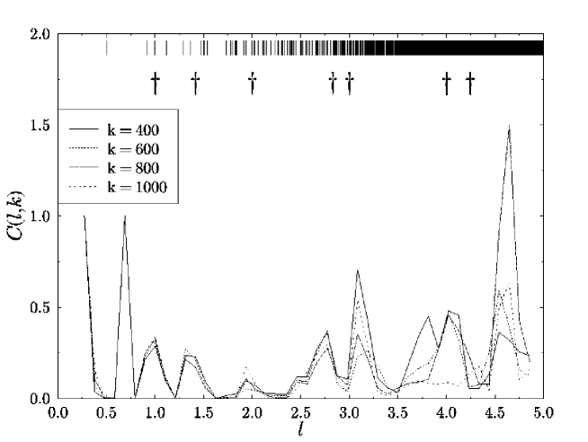
Figure 6: The functions $C(l;k)$ for quarter 2D Sinai billiard $L=1,R=0.25$ with Dirichlet boundary conditions. The window $w(k^{\prime}-k)$ was taken to be a Gaussian with standard deviation $\sigma=60$. We averaged $C(l;k)$ over $l$-intervals of $\approx 0.2$ in accordance with (36) to avoid sharp peaks due to small denominators. The averaging, however, is fine enough not to wash out all of the features of $C(l;k)$. The vertical bars indicate the locations of primitive periodic orbits, and the daggers indicate the locations of the bouncing–ball families.

Figure 7: Averaging in $l$ of $C(l;k)$ for 2D Sinai billiard as a function of $k$.

There are a few comments in order here. Firstly, the quarter desymmetrization of the 2D Sinai billiard does not exhaust its symmetry group, and in fact, a reflection symmetry around the diagonal of the square remains. This means, that the spectrum of the quarter 2D Sinai billiard is composed of two independent spectra, which differ by their parity with respect to the diagonal. If we assume that the semiclassical deviations of the two spectra are not correlated, the above measure is the sum of the two independent measures. It is plausible to assume also that both spectra have roughly the same semiclassical deviation, and thus $\delta^{\rm(2),2D}_{\rm smooth}$ is twice the semiclassical deviation of each of the spectra. Secondly, we recall that the 2D Sinai billiard contains “bouncing–ball” families of neutrally stable periodic orbits [37, 38, 32]. We have subtracted their leading-order contribution from $\hat{D}$ such that it includes (to leading order) only contributions from generic, isolated and unstable periodic orbits. This is done since we would like to deduce from the 2D Sinai billiard on the 2D generic case in which the bouncing–balls are not present. (In the Sinai billiard, which is concave, there are also diffraction effects [34, 13], but we did not treat them here.) Thirdly, the variant of (38) for billiards reads:

$$\left\langle\left|\hat{D}(l)\right|^{2}\right\rangle_{l}{\rm d}l=\frac{K(\xi)}{4\pi^{2}\xi^{2}}\ {\rm d}\xi$$ (47)

when $\xi\equiv l/L_{\rm H}$. In figure 8 we demonstrate the compliance of the form factor with RMT GOE using the integrated version of the above relation, and taking into account the presence of two independent spectra. Fourthly, it is interesting to know the actual numerical values of $\delta^{\rm(2),2D}_{\rm smooth}(k)$ for the $k$ values that we considered. We carried out the computation, and the results are presented in figure 9. It is interesting to observe, that for the entire range we have $\delta^{\rm(2),2D}_{\rm smooth}(k)\approx 0.1\ll 1$, which is very encouraging from an “engineering” point of view.

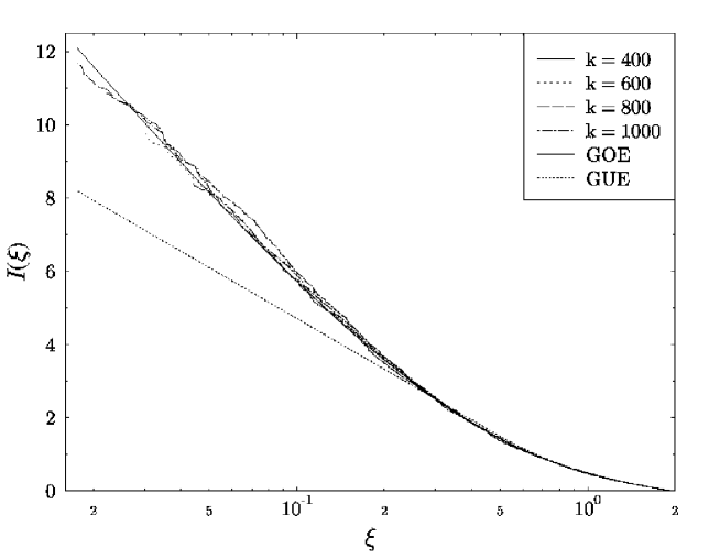
Figure 8: Verification of equation (47) for the quarter 2D Sinai billiard. We plot $I(\xi)\equiv\int_{\xi}^{2}{\rm d}\xi^{\prime}\ K(\xi^{\prime})/\xi^{\prime}\,{}^{2}$ and compare the quantum data with RMT. The minimal $\xi$ corresponds to $L_{\rm erg}=3.5$. The integration is done for smoothing, and we fix the upper limit to avoid biases due to non–universal regime. Note the logarithmic scale.

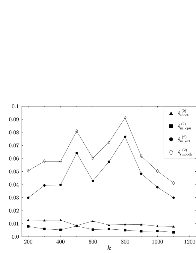
Figure 9: The numerical values of $\delta^{\rm(2)}_{\rm smooth}$ for the quarter 2D Sinai billiard. We included also the contribution $\delta^{\rm(2)}_{\rm short}$ of the non–universal regime. The contributions from the time interval $t_{\rm erg}\leq t\leq t_{\rm cpu}$ are contained in $\delta^{\rm(2)}_{\rm m,cpu}$, and $\delta^{\rm(2)}_{\rm m,ext}$ is the extrapolated value for $t_{\rm cpu}\leq t\leq t_{\rm H}$ (refer to (32) and to the end of section 2).

We now turn to the analysis of the 3D Sinai billiard. The billiard is the free space between a cube of edge $L$ and an inscribed sphere of radius $R$, where $2R<L$ (see figure 4). We used $L=1$ and $R=0.2$ and desymmetrized the billiard to the fundamental element (1/48 of the original one). We calculated the lowest 6697 quantum levels in the interval $0<k<281.1$ and the shortest 586965 periodic orbits with length $0<l<5$ (the number includes repetitions and time–reversal conjugates).

To treat the 3D Sinai billiard we need to somewhat modify the formalism which was presented in the previous section. This is due to the fact that in 3D the contributions of the various non–generic bouncing–ball manifolds overwhelm the spectrum [6, 7]. Since our goal is to give an indication of the semiclassical error in generic systems, it is imperative to get rid of this very strong non–generic effect. The bouncing ball amplitudes are ${\cal O}(k^{(s-1)/2})$ where $s$ is the dimensionality of bouncing–ball manifold in configuration space. In 3D $s=3$ typically, which completely overwhelms the contributions from isolated periodic orbits whose amplitude is ${\cal O}(k^{0})$. Even the diffraction corrections to the bouncing–ball amplitudes in 3D increase as ${\cal O}(k^{\gamma})$ with $\gamma>0$. In contrast with the 2D case, however, it is difficult to subtract the bouncing–ball contributions analytically for two main reasons. First, there are always infinitely many bouncing–ball primitive families in the 3D case, while in 2D there is only a finite number. Indeed, in any finite length interval there exists only a finite number of bouncing ball lengths, however their number for billiards in 3D exceeds by far the corresponding number for billiards in 2D. Second, the semiclassical amplitudes of the bouncing–balls are proportional to their volume in configuration space, and it is difficult in general to calculate it analytically. Thus, to overcome these difficulties we had to device a special method to cleanse the spectrum from the effect of the bouncing–balls and from the leading diffractive corrections. This method relies on the sensitivity of the eigenvalues to the boundary condition and it is described in detail in [39, 7]. We shall briefly describe the essence of the method.

The most general (“mixed”) boundary conditions under which the quantum billiard problem is self–adjoint can be written as [21, 39]:

$$\kappa\cos\alpha\,\psi(\vec{r}\,)+\sin\alpha\,\partial_{\vec{n}}\psi(\vec{r}\,)=0\mskip 5.0mu plus 5.0mu,\mskip 5.0mu plus 5.0mu\mskip 5.0mu plus 5.0mu\mskip 5.0mu plus 5.0mu\vec{r}\in(\mbox{boundary of the billiard})$$ (48)

where $\vec{n}$ is the normal pointing outside of the billiard, the angle $\alpha$ interpolates smoothly between Dirichlet ($\alpha=0$) and Neumann ($\alpha=\pi/2$) cases and $\kappa$ has the dimension of a wavenumber. Note that $\alpha$ and $\kappa$ can be different for different parts of the boundary. The spectrum depends parametrically on the boundary parameters, $\{k_{n}(\alpha,\kappa)\}$, and thus we can define the counting function $N(k;\alpha,\kappa)$. In [39, 7] we discussed the 2D and 3D Sinai billiards, and showed that if we choose Dirichlet boundary conditions on all the billiard boundaries excluding the circle (sphere), and set $\kappa\neq 0$ on the circle (sphere) then the quantity

$$\tilde{d}(k;\kappa)\equiv\left.\frac{\partial N(k;\alpha,\kappa)}{\partial\alpha}\right|_{\alpha=0}=\sum_{n}\left.\frac{\partial k_{n}(\alpha,\kappa)}{\partial\alpha}\right|_{\alpha=0}\delta(k-k_{n})\equiv\sum_{n}v_{n}\delta(k-k_{n})$$ (49)

is to a large extent free of the effects of the bouncing–balls. In the above $k_{n}\equiv k_{n}(\alpha=0)$ which are the Dirichlet–everywhere eigenvalues. The corresponding semiclassical trace formula reads [39, 7]:

$$\tilde{d}_{\rm sc}(k;\kappa)=(\mbox{smooth part})+\sum_{\rm po}A_{j}B_{j}\cos(kL_{j}-\nu_{j}\pi/2)$$ (50)

where

$$B_{j}=\frac{2k}{\kappa L_{j}}\sum_{i=1}^{n_{j}}\cos\theta_{i}^{(j)}.$$ (51)

In the above $n_{j}$ is the number of collisions with the circle (sphere) of the j’th periodic orbit, and $\{\theta_{i}^{(j)}\}$ are the angles of incidence on the boundary with respect to the normal. We note that (49) is a weighted density of states where the standard $1$ weights of the $\delta$ functions are replaced by $v_{n}$, and (50) is a weighted trace formula where the standard amplitudes $A_{j}$ are replaced by $A_{j}B_{j}$. One can show, that $B_{j}\approx v_{n}$ for long enough (ergodic) orbits.

We shall use $\tilde{d}$ for our purposes as follows. Let us consider the weighted counting function:

$$\tilde{N}(k)\equiv\int_{0}^{k}{\rm d}k^{\prime}\ \tilde{d}(k^{\prime})=\sum_{n}v_{n}\Theta(k-k_{n}).$$ (52)

The function $\tilde{N}$ is a staircase with stairs of variable height $v_{n}$. As was explained above, its advantage over $N$ is that it is semiclassically free of bouncing balls effects (to leading order) and corresponds only to the generic periodic orbits [39]. Similarly, we construct from $\tilde{d}_{\rm sc}$ the function $\tilde{N}_{\rm sc}$. Having defined $\tilde{N},\tilde{N}_{\rm sc}$, we proceed in analogy to the Dirichlet case. We form from $\tilde{N},\tilde{N}_{\rm sc}$ the functions $\hat{N},\hat{N}_{\rm sc}$, respectively, by multiplying with a window function $w(k^{\prime}-k)$ and then construct the measure $\delta^{\rm(2)}$ as in (25). The only difference is that the normalization of $w$ must be modified to account for the “velocities” $v_{n}$ such as:

$$\bar{d}^{-1}(k)\sum_{n}v_{n}^{2}|w(k_{n}-k)|^{2}=1.$$ (53)

The above considerations are meaningful provided that the “velocities” $v_{n}$ are narrowly distributed around a well-defined mean $v(k)$ and we consider a small enough $k$-interval, such that $v(k)$ does not change appreciably within this interval. Otherwise, $\delta^{\rm(2)}$ is greatly affected by the fluctuations of $v_{n}$ (which is undesired) and the meaning of the normalization is questionable.

To demonstrate the utility of the above construction using the mixed boundary conditions, we return to the 2D case. We set $\kappa=100\pi$, and note that the spectrum at our disposal for the mixed case was confined only to the interval $0<k<600$. First of all, we want to examine the width of the distribution of the $v_{n}$’s. In figure 10 we plot the ratio of the standard deviation of $v_{n}$ to the mean, averaged over the $k$-axis using a Gaussian window. We use the same window also in the calculations below. The observation is that the distribution of $v_{n}$ is moderately narrow and the width decreases algebraically as $k$ increases. This justifies the use of the mixed boundary conditions as was discussed above. One also needs to check the validity of (47), and indeed we found compliance with GOE also for the mixed case (results not shown). We next compare the functions $C(l;k)$ for both the Dirichlet and the mixed boundary conditions. It turns out, that also in the mixed case the functions $C(l;k)$ (not shown) fluctuate in $l$ with no special tendency. The averages $C_{\rm avg}(k)$ for the Dirichlet and mixed cases are compared in figure 11. The values in the mixed case are systematically smaller than in the Dirichlet case which is explained by the efficient filtering of tangent and close to tangent orbits that are vulnerable to large diffraction corrections [34, 13]. However, from $k=250$ on the two graphs show the same trends, and the values of $C_{\rm avg}$ in both cases are of the same magnitude. Thus, the qualitative behavior of $\delta^{\rm(2)}_{\rm smooth}$ is shown to be equivalent in the Dirichlet and mixed cases, which gives us confidence in using $\delta^{\rm(2)}_{\rm smooth}$ together with the mixed boundary conditions procedure.

Figure 10: Calculation of $Q\equiv\sqrt{\langle v_{n}^{2}\rangle-\langle v_{n}\rangle^{2}}/|\langle v_{n}\rangle|$ for quarter 2D Sinai billiard (up) and for the desymmetrized 3D Sinai billiard (down).

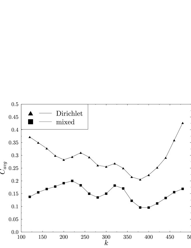
Figure 11: Comparison of $C_{\rm avg}(k)$ for Dirichlet and mixed boundary conditions for the quarter 2D Sinai billiard. We used a Gaussian window with $\sigma=40$.

We finally applied the mixed boundary conditions procedure to compute $\delta^{\rm(2)}_{\rm smooth}$ for the desymmetrized 3D Sinai with $L=1,R=0.2$ and set $\kappa=100$. We first verified that also in the 3D case the velocities $v_{n}$ have narrow distribution — see figure 10. Next, we examined equation (47) using quantal data, and discovered that there are deviations form GOE (figure 12). We have yet no satisfactory explanation of these deviations, but we suspect that they are caused because the ergodic limit is not yet reached for the length regime under consideration due to the effects of the infinite horizon which are more acute in 3D. Nevertheless, from observing the figure as well as suggested by semiclassical arguments, it is plausible to assume that $K(\xi)\propto\xi$ for small $\xi$. Hence, this deviation should not have any qualitative effect on $\delta^{\rm(2)}$ according to (41). Similarly to the 2D case, the behavior of the function $C(l;k)$ is fluctuative in $l$, with no special tendency (figure 13). If we average $C(l;k)$ over the universal interval $L_{\rm erg}=2.5\leq l\leq L_{\rm cpu}=5$, we obtain $C_{\rm avg}(k)$ which is shown in figure 14. The averages $C_{\rm avg}(k)$ are fluctuating with a mild decease in $k$, and therefore we can conclude that

$${\cal O}(k^{-\beta}\ln k)\leq\delta^{\rm(2),3D}_{\rm smooth}\leq{\cal O}(\ln k)$$ (54)

where the “optimistic” measure (leftmost term) corresponds to $C_{\rm avg}(k)={\cal O}(k^{-\beta}),\beta>0$, and the “pessimistic” one (rightmost term) is due to $C_{\rm avg}(k)={\rm const}$. In other words, the error estimates (46, 54) for the 2D and the 3D cases, respectively, are the same, and in sharp contrast to the “traditional” error estimate which predicts that the errors should be different by a factor ${\cal O}(\hbar^{-1})$. On the basis of our numerical data, and in spite of the uncertainties which were clearly delineated, we can safely exclude the “traditional” error estimate.

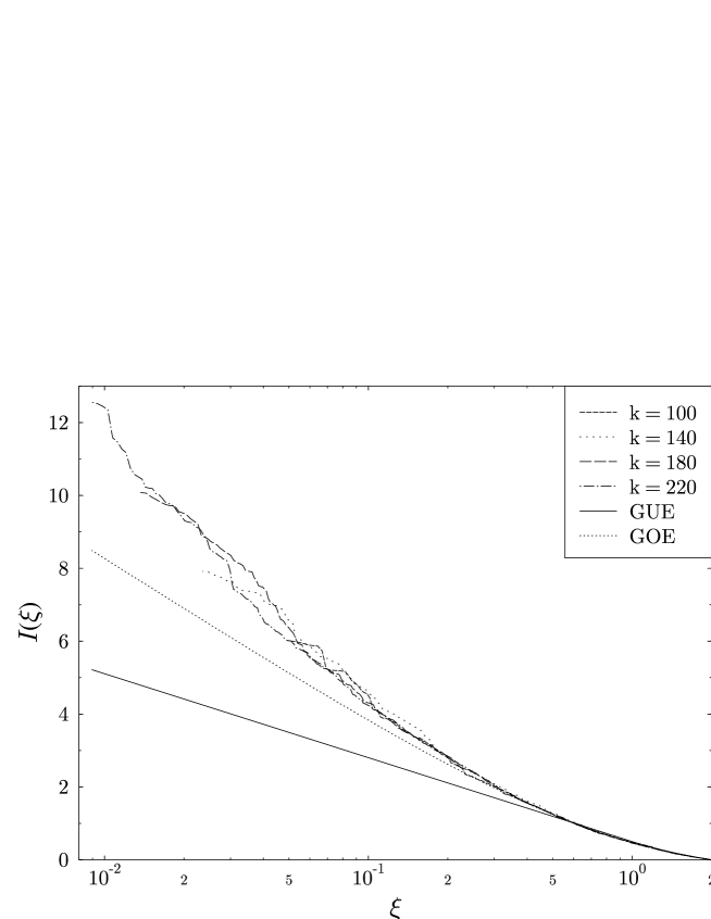
Figure 12: Check of equation (47) for the desymmetrized 3D Sinai billiard. The minimal $\xi$ corresponds to $L_{\rm erg}=2.5$. The function $I(\xi)$ is defined as in figure 8. Note the logarithmic scale.

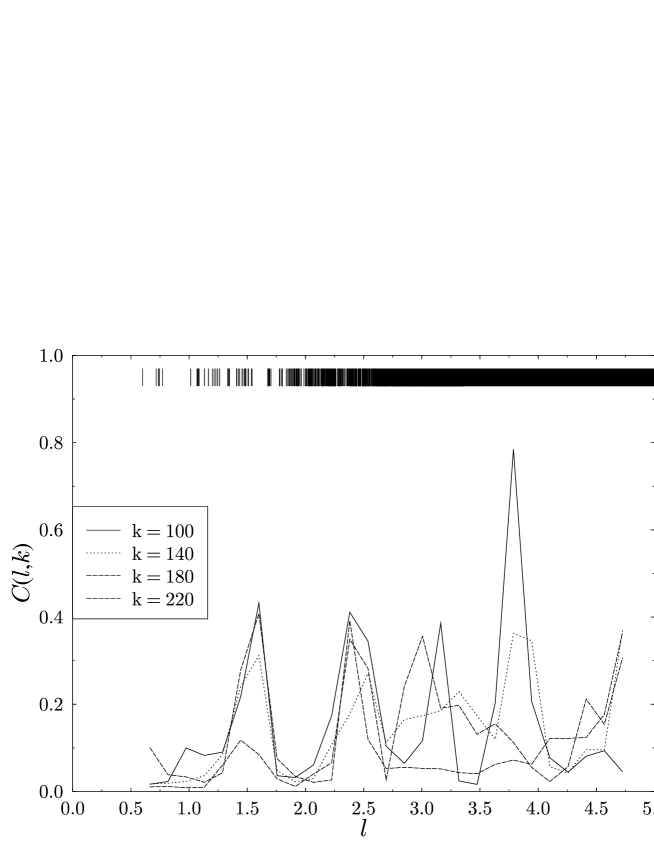
Figure 13: The functions $C(l;k)$ for desymmetrized 3D Sinai billiard $L=1,R=0.2$ with mixed boundary conditions. We took a Gaussian window with $\sigma=20$, and smoothed over $l$-intervals of $\approx 0.3$. The upper vertical bars indicate the locations of primitive periodic orbits.

Figure 14: Averaging in $l$ of $C(l;k)$ for 3D Sinai billiard as a function of $k$. The averaging was performed in the interval $L_{\rm erg}=2.5<l<5=L_{\rm cpu}$.

4 Discussion

Our main finding was that the upper bound on the semiclassical error is a logarithmic divergence, which is independent of the dimension (equations (46), (54)). In this respect, there are a few points which deserve discussion.

To begin, we shall try to evaluate $\delta^{\rm(2)}_{\rm smooth}$ using the explicit expressions for the leading corrections to the semiclassical counting function of 2D generic billiard system, as derived by Alonso and Gaspard [11]:

$$N(k)=\bar{N}(k)+\sum_{j}\frac{A_{j}}{L_{j}}\sin\left[kL_{j}+\frac{Q_{j}}{k}+{\cal O}(1/k^{2})\right]$$ (55)

where $A_{j}$ are the standard semiclassical amplitudes (see (30)), $L_{j}$ are the lengths of periodic orbits and $Q_{j}$ are the $k$-independent amplitudes of the $1/k$ corrections. The $Q_{j}$’s are given in [11]. We ignored in the above equation the case of odd Maslov indices. If we calculate from $N(k)$ the corresponding length spectrum $\hat{D}(l;k)$ using a (normalized) Gaussian window $w(k^{\prime}-k)=(1/\sqrt[4]{\pi\sigma^{2}})\exp[-(k^{\prime}-k)^{2}/(2\sigma^{2})]$, we obtain:

$$\hat{D}(l;k)\approx\frac{i\sqrt{\sigma}}{2\sqrt[4]{\pi}}\sum_{j}\frac{A_{j}}{L_{j}}\left[{\rm e}^{ik(l-L_{j})-i\frac{Q_{j}}{k}}{\rm e}^{-(l-L_{j})^{2}\frac{\sigma^{2}}{2}}-{\rm e}^{ik(l+L_{j})+i\frac{Q_{j}}{k}}{\rm e}^{-(l+L_{j})^{2}\frac{\sigma^{2}}{2}}\right].$$ (56)

In the above we regarded the phase ${\rm e}^{iQ_{j}/k}$ as slowly varying. The results of Alonso and Gaspard [11] suggest that the $Q_{j}$ are approximately proportional to the length of the corresponding periodic orbits:

$$Q_{j}\approx QL_{j}.$$ (57)

We can therefore well–approximate $\hat{D}$ as:

$$\hat{D}(l;k)\approx\frac{i\sqrt{\sigma}}{2\sqrt[4]{\pi}}{\rm e}^{-iQl/k}\sum_{j}\frac{A_{j}}{L_{j}}\left[\cdots\right]={\rm e}^{-iQl/k}\hat{D}_{\rm sc-GTF}\,,$$ (58)

where $\hat{D}_{\rm sc-GTF}$ is the length spectrum which corresponds to the semiclassical Gutzwiller trace formula for the counting function (without $1/k$ corrections). We are now in a position to evaluate the semiclassical error, indeed:

$$\delta^{\rm(2)}_{\rm smooth}(k) = 2\int_{L_{\rm min}}^{L_{\rm H}}{\rm d}l\left|\hat{D}(l;k)-\hat{D}_{\rm sc-GTF}(l;k)\right|^{2}=$$ (59)

$$= 8\int_{L_{\rm min}}^{L_{\rm H}}{\rm d}l\,\sin^{2}\left(\frac{Ql}{2k}\right)\left|\hat{D}(l;k)\right|^{2}\,.$$

If we now use equation (47) and $K(l)\approx gl/L_{\rm H}$ (which is valid for $l<L_{\rm H}$ for chaotic systems), we get:

$$\delta^{\rm(2)}_{\rm smooth}(k)\approx\frac{2g}{\pi^{2}}\int_{L_{\rm min}}^{L_{\rm H}}\frac{{\rm d}l}{l}\sin^{2}\left(\frac{Ql}{2k}\right)=\frac{2g}{\pi^{2}}\int_{QL_{\rm min}/(2k)}^{QL_{\rm H}/(2k)}{\rm d}t\frac{\sin^{2}(t)}{t}\,.$$ (60)

For $k\rightarrow\infty$ we have that

$$\int_{0}^{QL_{\rm min}/(2k)}{\rm d}t\frac{\sin^{2}(t)}{t}\approx\int_{0}^{QL_{\rm min}/(2k)}{\rm d}t\cdot t={\cal O}(1/k^{2})$$ (61)

which is negligible, hence we can replace the lower limit in (60) with 0:

$$\delta^{\rm(2)}_{\rm smooth}(k)\approx\frac{2g}{\pi^{2}}\int_{0}^{\frac{QL_{\rm H}}{2k}}{\rm d}t\frac{\sin^{2}(t)}{t}\,.$$ (62)

This is the required expression. The dimensionality enter in $\delta^{\rm(2)}_{\rm smooth}(k)$ only through the power of $k$ in $L_{\rm H}$.

Let us apply equation (62) to 2D and 3D cases. For 2D we have that $L_{\rm H}=Ak$ in leading order, where $A$ is the billiard’s area, thus,

$$\delta^{\rm(2),2D}_{\rm analytical}(k)\approx\frac{2g}{\pi^{2}}\int_{0}^{QA/2}{\rm d}t\frac{\sin^{2}(t)}{t}={\rm const}={\cal O}(k^{0})$$ (63)

which means, that the semiclassical error in 2D billiards is of the order of the mean spacing, and therefore the semiclassical trace formula is (marginally) accurate and meaningful. This is compatible with our numerical findings within the limitations of the numerical fluctuations.

For 3D, the coefficients $Q_{j}$ were not obtained explicitly, but we shall assume that they are still proportional to $L_{j}$ (equation (57)) and thus that (62) holds. For 3D billiards $L_{\rm H}=(V/\pi)k^{2}$ to leading order, where $V$ is the billiard’s volume. Thus the upper limit in (62) is $QVk/(2\pi)$ which is large in the semiclassical limit. In that case, we can replace $\sin^{2}(t)$ with its mean value $1/2$ and the integrand becomes essentially $1/t$ which results in:

$$\delta^{\rm(2),3D}_{\rm analytical}(k)={\cal O}(\ln k)\,.$$ (64)

That is, in contrast to the 2D case, the semiclassical error diverges logarithmically and the semiclassical trace formula becomes meaningless as far as the prediction of individual levels is concerned. This is compatible with our numerical results within the numerical dispersion. However, it relies heavily on the assumption that $Q_{j}\approx QL_{j}$, for which we can offer no justification. We note in passing, that the logarithmic divergence persists also for $d>3$.

Another interesting point relates to integrable systems. It can happen, that for an integrable system it is either difficult or impossible to express the Hamiltonian as an explicit function of the action variables. In that case, we cannot assign to the levels other quantum numbers than their ordinal number, and the semiclassical error can be estimated using $\delta^{\rm(2)}$. However, since for integrable systems $K(\tau)=1$, we get that:

$$\delta^{\rm(2),int}_{\rm smooth}\approx\frac{1}{2\pi^{2}}\int_{\tau_{\rm erg}}^{1}{\rm d}\tau\,\frac{C(\tau)}{\tau^{2}}.$$ (65)

Therefore, for deviations which are comparable to the chaotic cases, $C(\tau)={\cal O}(1)$, we get $\delta^{\rm(2),int}_{\rm smooth}={\cal O}(\hbar^{1-d})$ which is much larger than for the chaotic case and diverges for $d\geq 1$.

The formula (41) for the semiclassical error contains semiclassical information in two respects. Obviously, $C(\tau)$, which is the difference between the quantal and the semiclassical length spectra contains semiclassical information. But also, the fact that the lower limit of the integral in (41) is finite is a consequence of semiclassical analysis. If this lower limit is replaced by $0$, the integral diverges for finite values of $\hbar$, which is meaningless. Therefore, the fact that the integral has a lower cutoff, or rather, that $D$ is exactly $0$ below the shortest period, is a crucial semiclassical ingredient in our analysis.

Finally, we consider the case in which the semiclassical error is estimated with no periodic orbits taken into account. That is, we want to calculate $\langle|N(E)-\bar{N}(E)|^{2}\rangle_{E}$ which is the number variance $\Sigma^{2}(x)$ for the large argument $x=\Delta E\,\bar{d}(E)\gg 1$. This implies $C(\tau)=1$, and using (41) we get that $\delta^{\rm(2)}_{\rm smooth}=g/(2\pi^{2})\ln(t_{\rm H}/t_{\rm erg})$, which in the semiclassical limit becomes $g/(2\pi^{2})\ln(t_{\rm H})={\cal O}(\ln\hbar)$. This result is fully consistent and compatible with previous results for the asymptotic (saturation) value of the number variance $\Sigma^{2}$ (see for instance [29, 40, 41]). It implies also that the pessimistic error bound (44) is of the same magnitude as if periodic orbits were not taken into account at all. (Periodic orbits improve, however, quantitatively, since in all cases we obtained $C_{\rm avg}<1$.) Thus, if we assume that periodic orbit contributions do not make $N_{sc}$ worse than $\bar{N}$, then the pessimistic error bound ${\cal O}(\ln\hbar)$ is the maximal one in any dimension $d$. This excludes, in particular, algebraic semiclassical errors, and thus refutes the traditional estimate ${\cal O}(\hbar^{2-d})$.

References

References

- [1] M. C. Gutzwiller. Chaos in Classical and Quantum Mechanics. Springer–Verlag, New York, 1990.
- [2] M. V. Berry. Semiclassical theory of spectral rigidity. Proc. Roy. Soc. London A, 400:229, 1985.
- [3] E. B. Bogomolny and J. P. Keating. Gutzwiller’s trace formula and spectral statistics: Beyond the diagonal approximation. Phys. Rev. Lett., 77(8):1472–1475, 1996.
- [4] L. D. Landau and E. M. Lifshitz. Quantum mechanics, non-relativistic theory, volume 3 of Course of theoretical physics. Pergamon Press, 1958.
- [5] W. Pauli. Ausgewählte Kapital aus der Feldquantisierung. In C. Enz, editor, Lecture notes, Zürich, 1951.
- [6] Harel Primack and Uzy Smilansky. Quantization of the three-dimensional Sinai billiard. Phys. Rev. Lett., 74(24):4831–4834, 1995.
- [7] Harel Primack. Quantal and semiclassical analysis of the three–dimensional Sinai billiard. PhD thesis, The Weizmann Institute of Science, Rehovot, Israel, 1997. Submitted for refereeing.
- [8] Tomaz Prosen. Quantization of generic chaotic 3d billiard with smooth boundary I: Energy level statistics. Phys. Lett. A, 233:323–331, 1997.
- [9] Martin C. Gutzwiller. The semi-classical quantization of chaotic hamiltonian systems. In M.-J. Giannoni, A. Voros, and J. Zinn-Justin, editors, Proceedings of the 1989 Les Houches Summer School on “Chaos and Quantum Physics”, pages 201–249. Elsevier Science Publishers B.V., Amsterdam, 1991.
- [10] P. Gaspard and D. Alonso. expansion for the periodic orbit quantization of hyperbolic systems. Phys. Rev. A, 47(5):R3468–R3471, 1993.
- [11] D. Alonso and P. Gaspard. expansion for the periodic orbit quantization of chaotic systems. CHAOS, 3(4):601–612, 1993.
- [12] Gabor Vattay, Andreas Wirzba, and Per E. Rosenqvist. Periodic orbit theory of diffraction. Phys. Rev. Lett., 73:2304, 1994.
- [13] Harel Primack, Holger Schanz, Uzy Smilansky, and Iddo Ussishkin. Penumbra diffraction in the semiclassical quantization of concave billiards. J. Phys. A, 30:6693–6723, 1997.
- [14] P. A. Boasman. Semiclassical accuracy for billiards. Nonlinearity, 7:485–533, 1994.
- [15] M. V. Berry and M. Wilkinson. Diabolical points in the spectra of triangles. Proc. R. Soc. A, 392:15–43, 1984.
- [16] P. M. Bleher. Quasi-classical expansions and the problem of quantum chaos. In Geometric aspects of functional analysis, Proc. Isr. Semin., GAFA, Isr. 1989-90, Lect. Notes Math., pages 60–89. Springer, 1991.
- [17] P. M. Bleher. Distribution of energy levels of a quantum free particle on a surface of revolution. Duke Math. Jour., 74(1):45–93, 1994.
- [18] T. Prosen and M. Robnik. Failure of semiclassical methods to predict individual energy levels. J. Phys. A, 16:L37–L44, 1993.
- [19] R. Aurich and J. Marklof. Trace formulae for three–dimensional hyperbolic lattice and application to a strongly chaotic tetrahedral billiard. Physica D, 92:101–129, 1996.
- [20] J. P. Keating. The Riemann Zeta function and quantum chaology. In G. Casati, I. Guarnery, and U. Smilansky, editors, Proceedings of the 1991 Enrico Fermi International School on “Quantum Chaos”, course CXIX. North-Holland, 1993.
- [21] R. Balian and B. Bloch. Distribution of eigenfrequencies for the wave equation in a finite domain I. Three–dimensional problem with smooth boundary surface. Ann. Phys., 60:401–447, 1970.
- [22] H. P. Baltes and E. R. Hilf. Spectra of Finite Systems. Bibliographisches Institut, Mannheim, 1976.
- [23] M. V. Berry and C. J. Howls. High orders of the Weyl expansion for quantum billiards: Resurgence of the Weyl series, and the Stokes phenomenon. Proc. Roy. Soc. Lond. A, 447(1931):527–555, 1994.
- [24] E. Doron and U. Smilansky. Semiclassical quantization of chaotic billiards — a scattering theory approach. Nonlinearity, 5:1055–1084, 1992.
- [25] E. B. Bogomolny. Semiclassical quantization of multidimensional systems. Nonlinearity, 5:805, 1992.
- [26] B. Georgeot and R. E. Prange. Exact and quasiclassical Fredholm solutions of quantum billiards. Phys. Rev. Lett., 74(15):2851–2854, 1995.
- [27] M. Sieber. The Hyperbola Billiard: A Model for the Semiclassical Quantization of Chaotic Systems. PhD thesis, University of Hamburg, 1991. DESY preprint 91-030.
- [28] Takahisa Harayama and Akira Shudo. Periodic orbits and semiclassical quantization of dispersing billiards. J. Phys. A, 25:4595–4611, 1992.
- [29] M. V. Berry. Some quantum to classical asymptotics. In M.-J. Giannoni, A. Voros, and J. Zinn-Justin, editors, Proceedings of the 1989 Les Houches Summer School on “Chaos and Quantum Physics”, page 251. Elsevier Science Publishers B.V., Amsterdam, 1991.
- [30] K. G. Andersson and R. B. Melrose. The propagation of singularities along gliding rays. Inventiones Math., 41:197–232, 1977.
- [31] O. Bohigas, M. J. Giannoni, and C. Schmit. Characterization of chaotic quantum spectra and universality of level fluctuations. Phys. Rev. Lett., 52(1):1–4, 1984.
- [32] H. Schanz and U. Smilansky. Quantization of Sinai’s billiard – A scattering approach. Chaos, Solitons and Fractals, 5(7):1289–1309, 1995.
- [33] Holger Schanz. Investigation of Two Quantum Chaotic Systems. PhD thesis, Humboldt University Berlin, 1997. LOGOS Verlag, Berlin (1997).
- [34] Harel Primack, Holger Schanz, Uzy Smilansky, and Iddo Ussishkin. Penumbra diffraction in the quantization of dispersing billiards. Phys. Rev. Lett., 76(10):1615–1618, 1996.
- [35] A. J. Fendrik and M. J. Sanchez. Decay of the Sinai well in dimensions. Phys. Rev. E, 51:2996, 1995.
- [36] Per Dahlqvist and Roberto Artuso. On the decay of correlations in Sinai billiards with infinite horizon. Phys. Lett. A, 219:212–216, 1996.
- [37] M. V. Berry. Quantizing a classically ergodic system: Sinai billiard and the KKR method. Ann. Phys., 131:163–216, 1981.
- [38] M. Sieber, U. Smilansky, S. C. Creagh, and R. G. Littlejohn. Non-generic spectral statistics in the quantized stadium billiard. J. Phys. A, 26:6217–6230, 1993.
- [39] Martin Sieber, Harel Primack, Uzy Smilansky, Iddo Ussishkin, and Holger Schanz. Semiclassical quantization of billiards with mixed boundary conditions. J. Phys. A, 28:5041–5078, 1995.
- [40] E. Bogomolny and C. Schmit. Semiclassical computations of energy levels. Nonlinearity, 6:523–547, 1993.
- [41] R. Aurich, J. Bolte, and F. Steiner. Universal signatures of quantum chaos. Phys. Rev. Lett., 73:1356–1359, 1994.