ESS and Dissipation Range Dynamics of 3-D Turbulence

Abstract

We carry out a self consistent calculation of the structure functions in the dissipation range using Navier Stokes equation. Combining these results with the known structures in the inertial range, we actually propose crossover functions for the structure functions that takes one smoothly from the inertial to the dissipation regime. In the process the success of the extended self similarity is explicitly demonstrated.

The inertial range of fully developed homogeneous, isotropic turbulece has been investigated extensively [1-8] in the past decade. In comparison far dissiaption range is been less well studied and as far as we know, a systematic study of the structure functions, based on Navier Stokes equation (NS), has not been carried out. In this work, we report a self consistent calculation of the structure functions in the dissipation range. Using accepted results in the inertial range, we propose crossover functions for the structure functions and thus demonstrate how extended self similarity can be understood.

We work with forced three dimensional NS equation for incompressible flows, written in the momentum space as,

$$\dot{v}_{i}({\bf k})+\nu k^{2}v_{i}({\bf k})=\frac{-i}{2}M_{ijl}({\bf k})\sum_{\bf p}v_{j}({\bf p})v_{l}({\bf k-p})+f_{i}({\bf k},t)$$ (1)

Where $M_{ijl}=k_{j}P_{il}({\bf k})+k_{l}P_{ij}({\bf k})\/$ and the transverse projector, $P_{ij}=\delta_{ij}-k_{i}k_{j}/{k^{2}}\/$, where the external noise $f_{i}\/$ is $\delta\/$ correlated and is necessary to maintain the energy balance in the inertial range. The energy input per unit time ($\bar{\epsilon}\/$) at the long wave lengths cascades through different lenght scales due to the nonlinear term and for $k>k_{D}\/$, is dissipated by molecular viscosity ($\nu\/$), here $k_{D}=(\bar{\epsilon}/\nu^{3})^{1/4}\/$. For ($k<<k_{D}\/$), we have the so called inertial range, where one expects,

$$S_{2n}\sim k^{-(\zeta_{2n}+3n)}$$ (2)

with structure function defined as in Dhar et al [9] as, $S_{n}=\langle|v(k)|^{n}\rangle\/$. The exponent $\zeta_{n}\/$ is $n/3\/$ in the Kolmogorov limit. In general it differs from $n/3\/$ and one of the best estimates of the deviation is due to She and Leveque [10] which gives,

$$\delta\zeta_{n}=\zeta_{n}-n/3=-\frac{2n}{9}+2[1-(\frac{2}{3})^{n/3}]$$ (3)

In this work we investigated the dissipation range and our principal results are

$$S_{2n}(k)\sim k^{n\delta_{2}}e^{-nk/K},\;\;\;\;(k>>K)$$ (4)

where $\delta_{2}=2-D\/$ (D being the dimensionality of space) and $K=\Theta(k_{D})\/$. By studying the correction to the above result as powers of $K/k\/$, we propose (in $D=3\/$) the crossover function (crossover from dissipation to inertial range)

$$S_{2}(k)\sim\frac{1}{k}(1+\alpha_{1}\frac{K}{k})^{2+\zeta_{2}}e^{-k/K}$$ (5)

where $\alpha_{1}\/$ is number of $\Theta(1)\/$, while for higher order structure function,

$$S_{2n}(k)\sim k^{n\delta_{2}}(1+\alpha_{n}\frac{K}{k})^{n(3+\delta_{2})+\zeta_{2n}}e^{-nk/K}$$ (6)

The constants $\alpha_{n}\/$ are non-universal but will be shown to be almost independent of $n\/$. The explicit crossover forms that we have written down helps us understand the idea of extended self similarity (ESS) introduced by Benzi et al[11]. Our approach is alternative to that of Segel et al[13]. Writing Eq.6 by expanding about the inertial range form, we note that,

$$S_{2n}(k)\sim k^{-(\zeta_{2n}+3n)}(1-[n-\frac{n(3+\delta_{2})+\zeta_{2n}}{\alpha_{n}}]\frac{k}{K})$$ (7)

the simple power law will break down when,

$$k\sim\frac{\alpha_{n}}{n(\alpha_{n}-3-\delta_{2})-\zeta_{2n}}K$$ (8)

From phenomenology, it is known that $S_{n}\/$ falls off from the $k^{-(\zeta_{2n}+3n)}\/$ line in the dissipation range. This constrains $\alpha_{n}\/$ (from Eq 7 and using $\delta_{2}=2-D\/$),

$$\frac{n(\alpha_{n}-2)-\zeta_{2n}}{\alpha_{n}}>0$$ (9)

Now if we assume $\alpha_{n}>0\/$ and use the fact that $\alpha_{n}\/$ is almost independent of $n\/$ (shown later), we get,

$$\alpha_{1}>2+\zeta_{2}$$ (10)

As $\alpha_{n}-2>\zeta_{2}(=2/3)\/$, the difference $n(\alpha_{n}-2)-\zeta_{2n}\/$ will grow with $n\/$ (since we know that $\zeta_{2n}\/$ deviates more from linearity for higher moments). Hence for higher $n\/$ the $S_{n}\/$ curves will fall off from the scaling regime at even lower $k\/$ values. This is completely consistent with the standard phenomenology [15].

We now turn to ESS. From Eq.6 it is clear that,

$$S_{2n}(k)\sim [ S_{2m}(k)]^{(\frac{\zeta_{2n}+3n}{\zeta_{2m}+3m})}e^{-nk/K}e^{m(\frac{\zeta_{2n}+3n}{\zeta_{2m}+3m})k/K}$$ (13)

$$\times\frac{[1+\alpha_{n}^{-1}\frac{k}{K}]^{n(3+\delta_{2})+\zeta_{2n}}}{[1+\alpha_{m}^{-1}\frac{k}{K}]^{(m(3+\delta_{2})+\zeta_{2m})(\frac{\zeta_{2n}+3n}{\zeta_{2m}+3m})}}$$

The explicit $k\/$ dependant terms on the r.h.s. of the above expression will cause deviation from scaling. But it is apparent that the exponential factor is much more weakly decaying than $e^{-nk/K}\/$ (in fact it is constant for the Kolmogorov situation of $\zeta_{2n}=2n/3\/$) and also the variation of $[1+\alpha_{n}^{-1}\frac{k}{K}]^{n(3+\delta_{2})+\zeta_{2n}}\/$ is muted by the denominator (as $\alpha_{n}\/$s’ have been assumed to have the same sign and shown to be almost independent later). Consequently a plot of $\log S_{2n}\;\/$ vs $\;\log S_{2m}\/$ will remain a straight line over a far longer range than $S_{2n}\;\/$ vs $\;k^{-(\zeta_{2n}+3n)}\/$. This is the content of ESS. Few other phenomenological consequences are also manifest. For example, as $(n-m)\/$ grows the scaling regime will become gradually shorter. In fact with $\alpha_{n}\/$ independent of $n\/$ to a first approximation and $\zeta_{2n}\/$ almost proportional to $n\/$, the scaling of $\log S_{2n}\;\/$ vs $\;\log S_{2m}\/$ is virtually exact.

We first note that correlation functions in the dissipation range falls off extremely fast [12] with the characteristic scale $k_{D}\/$ and because of the existance of the scale there is no divergence in the self energies and correlation functions. Absence of divergence in the self energy implies that vicosity coefficient $\nu\/$ is not renormalised. The correlation function is given at the self consistent single loop level by,

$$S_{2}(k,w)=|G|^{2}k^{2} \int \frac{d^{D}p}{(2\pi)^{D}}\frac{dw^{\prime}}{2\pi}a({\bf k,p,k-p})$$ (15)

$$\times S_{2}(|{\bf k-p}|,w-w^{\prime})S_{2}(p,w^{\prime})$$

where the angular factor,

$$a({\bf k,p,k-p})=\frac{1}{2}(1-xyz-2y^{2}z^{2})$$ (16)

The trio $({\bf k,p,k-p})\/$ forms a triangle and $x,y,z\/$ are the direction cosines of the angles opposite to ${\bf k,p}\/$ and ${\bf k-p}\/$ respectively. The response function $G^{-1}=-iw+\nu k^{2}\/$ and the correlation function $S_{2}(k,w)=k^{\delta_{2}}f(k/k_{D})k^{2}/(w^{2}+\nu^{2}k^{4})\/$, such that

$$\int\frac{dw}{2\pi}S_{2}(k,w)=S_{2}(k,t=0)=k^{\delta_{2}}f(k/k_{D})$$ (17)

Comparing the two sides of Eq.9, the function $f(k/k_{D})\/$ has the structure $f(k/k_{D})=e^{-\beta k/k_{D}}\/$, since on the right hand side of Eq.9,

$$e^{-\beta p/k_{D}}e^{-\beta|{\bf k-p}|/k_{D}} = e^{-\beta({\bf|\frac{k}{2}-q|+|\frac{k}{2}+q|})/k_{D}}$$ (18)

$$= e^{-\beta k/k_{D}}(e^{-\Theta(q^{2}/k^{2})}+\ldots)$$ (19)

$$\simeq e^{-\beta k/k_{D}}$$ (20)

thus reproducing the exponential factor of the left hand side. Power counting of the momentum in Eq.9 now leads to,

$$\delta_{2}=-(D-2)$$ (21)

To check the correctness of this self consistent solution we avaluated the equal time limit of the integral on the r.h.s. of eqn.9 numerically (with lower cutoff $k_{D}\/$ and $D=3\/$). In fig.1(a) we plot this integral $I_{d}(k)\/$ and compare it with the function $\frac{1}{k}e^{-k/k_{D}}\/$. The agreement is good for $k/{k_{D}}\geq 20\/$ (ie, $k>>{k_{D}}\/$).

If the above formalism has to approach the crossover behaviour, then we need to include the first correction to the large $k\/$ behaviour. We do this by saying that the correction is in powers of $(K/k)^{m}\/$ and thus in $D=3\/$

$$S_{2}=\frac{b_{0}}{k}[1+b_{1}(K/k)^{m}]e^{-k/K}$$ (22)

where $K=k_{D}/\beta\/$. The right hand side of Eq.9, linearised in $b_{1}\/$ and considered at zero frequency can be written as being proportional to:

$$\int \frac{d^{3}p}{(2\pi)^{3}}a({\bf k,p,k-p})\frac{e^{-(p+|{\bf k-p}|)/K}}{(p^{2}+|{\bf k-p}|^{2})p|{\bf k-p}|}$$ (24)

$$\times[1+b_{1}(K/p)^{m}+b_{1}(K/|{\bf k-p}|)^{m}]$$

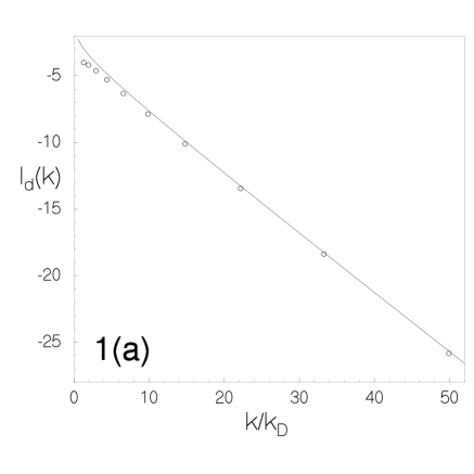
FIG. 1.: The dominant $\Theta({b_{1}}^{0})\/$ and correction $\Theta(b_{1})\/$ terms in eq.14, obtained from numerical integration (circle ’o’) are compared with the respective terms (solid line) in eqn.13. (a)circle: $log_{10}I_{d}(k)\/$ ; solid: $\frac{b_{0}}{k}e^{-k/k_{D}}\/$ (b) $log_{10}I_{c}(k)\/$ ; solid: $\frac{b_{0}}{k}({k_{D}}/k)^{1/4}e^{-k/k_{D}}\/$.

The requirement that the integral involving $b_{1}\/$ is finite, leads to $m<2\/$. If we write $m=2-\epsilon\/$, we can evaluate the integrals to the leading pole [14] in $\epsilon\/$. The integral not involving $b_{1}\/$ can be evaluated using saddle point technique, with dominant contribution coming from $p\simeq k\/$. The result of the above manipulation must be of the form $[1+b_{1}(K/p)^{m}]\/$ for self consistency and at the level of approximation just described, we find $m=1\/$. Thus, we have the result that for $k>>k_{D},\;\;S_{2}\propto\frac{1}{k}(1+b_{1}\frac{K}{k})e^{-k/K}\/$ and for $k<<k_{D}\/$ (inertial range), $S_{2}\propto k^{-(3+\zeta_{2})}\/$. The simplest interpolation is Eq.5.

Using the above analysis as a guide towards determining $m\/$, we numerically evaluated the correction integral $I_{c}(k)\/$ of $\Theta(b_{1})\/$ in eqn.14. Using the same values of $b_{0}\/$ and the lower cutoff $k_{D}\/$ which we had used for fitting the dominant term, we find self consistency of the correction integral can be achieved for $m\simeq 1/4\/$. In fig.1(b) we plot this integral $I_{c}(k)\/$ as a function of $k/{k_{D}}\/$ and compare it with the $\Theta(b_{1})\/$ term in eqn.13. The agreement is good for $k/{k_{D}}\geq 7\/$. We have chosen $K={k_{D}}\/$ for our numerics. All our arguments demonstrating the ESS properties of $S_{n}\/$ hold good as long as $m>0\/$.

It should be noted that in this far dissipation range that we are considering here, the single loop self consistency is sufficient. We have checked that the contributions from higher ($\geq 2\/$) loop diagrams are at most of the same order as the single loop diagram. So their inclusion just changes the amplitude of $S_{2}(k)\/$. This statement is true for the evaluation of $S_{2n}\/$ ($n>1\/$) also, which we do now. Out of the various possible arrangements of the ${\bf k}\/$ and ${\bf-k}\/$ external legs on an one loop diagram, we evaluate the most relevant one (shown in Fig.1). Contribution from other possible one loop diagrams are exponentially smaller and hence their contributions are negligible. The contribution from Fig.1 is,

$$S_{2n}(k,t) = \langle[v({\bf k},t)v({\bf-k},t)]^{n}\rangle$$ (25)

$$\sim k^{2n}\int_{-\infty}^{t}dt_{1}\ldots\int_{-\infty}^{t}dt_{2n}\int\frac{d^{D}p}{(2\pi)^{D}}$$ (28)

$$\times G(k;t,t_{1})G(-k;t,t_{2})\ldots$$

$$\times S_{2}(p,|t_{1}-t_{2}|)S_{2}(|{\bf k-p}|,|t_{2}-t_{3}|)\ldots$$

As $S_{2}(k,t)\sim k^{-(D-2)}e^{-k/K}e^{-|t|\nu k^{2}}\/$, we note that the integral of Eq.15 will be dominated by the low momentum pole at $p=k\/$. Using a pole approximation for evaluating the integral, a momentum count produces the result that $S_{2n}(k,t)\propto k^{n\delta_{2}}e^{-nk/K}\/$ . This establishes Eq 4. However, within this formalism, though we cannot rigorously show that Eq.4 holds for odd moments also, for monotonicity sake we assume this to be true. Now we note that Eq 4 implies $S_{n}\sim S_{3}^{n/3}\/$ ie, simple scaling behaviour results in the far dissipation range. This is in mild contrast to the simulation results [9], where very weak multiscaling (ie, very small deviation from $n/3\/$) has been reported. But given that this deviation is very small, e.g. for $n=7\/$ the numerical exponent is 2.24 instead of 7/3, our estimate for this far dissipation range is a very close one.

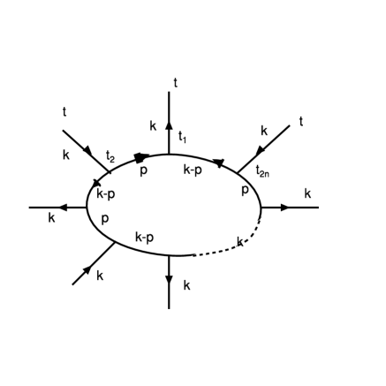
FIG. 2.: Diagram contributing to $S_{2n}(k)\/$ in the dissipation regime

We now study the first deviation of $S_{2n}\/$ from its form in Eq 4. To do so, we introduce the first deviation of $S_{2n}(k,t)\/$ in Eq 15. The integral in in Eq.15 is already pole dominated and hence the additional part is pole dominated as well. There are $n\/$ contributions of equal strength from each of the $S_{2}(p)\/$ and $S_{2}(|{\bf k-p}|)\/$ and consequently for $k>>K\/$

$$S_{2n}\propto k^{-n(D-2)}[1+b_{n}(K/k)]e^{-nk/K}$$ (29)

where $b_{n}\propto nb_{1}\/$. With the quantity $n(3+\delta_{2})+\zeta_{2n}\/$ in Eq.6 roughly proprtional to $n\/$, we consequently infer that in the interpolation formula of Eq.6, the constant $\alpha_{n}\/$ is to a good approximation independent of $n\/$. Thus the main results Eq.4 - Eq6, are obtained.

Now we look at the real space structure function $S_{2}(r)=\langle[{\bf v}({\bf x}+{\bf r})-{\bf v}({\bf x})]^{2}\rangle\/$ which is the inverse Fourier transform of $2[{u_{0}}^{2}\delta(k)-S_{2}(k)]\/$ (where ${{u_{0}}^{2}}/2\/$ is the mean energy). For $r\/$ in the far dissipation range $S_{2}(r)\/$ will be determined by our $k>>k_{d}\/$ form of $S_{2}(k)\/$ (ie,$\sim\frac{1}{k}e^{-k/K}\/$). This yields $S_{2}(r)=c_{1}r^{2}+\Theta(r^{4})\/$. Here $c_{1}\/$ is a function of $\nu,\bar{\epsilon}\/$. This form of $S_{2}(r)\/$ is consistent with the result of Sirovich et.al.[16]. The added advantage of our $k-\/$ space calculation is the ability to predict the higher order structure functions ($S_{2n}(k)\/$) also.

In summary we have shown that by considering Navier Stokes equation and doing a self consistent treatment of the dissipation range (characterised by the existence of a scale $k_{D}\/$ ), we can establish forms for the various order structure functions. By the first correction to the asymtotic situation and using the known results in the inertial range ($k<<k_{D}\/$), we can construct explicit crossover functions for the structure functions (crossover from $k>>k_{D}\/$ to $k<<k_{D}\/$ ). The validity of ESS is easy to see.

We would like to thank R.Pandit for comments, P.Pradhan for help in drawing the Feynman diagram (fig.2) and CSIR (India) for support.

REFERENCES

[1] U. Frish,Turbulence : The Legacy of
A.N. Kolmogorov (Cambridge Univ. Press, Cambridge, 1995).
[7] V. Yakhot and S.A.Orszag,J. Sci. Comput.,
1, 3 (1986).
[8]Sujan K. Dhar, Anirban Sain,Ashwin Pande,
and Rahul Pandit Pramana: Indian J. Phys. (Special issue
on Nonlinrity and Chaos in Physical Sciences),48,
325 (1997)
[9],Sujan K. Dhar, Anirban Sain and Rahul Pandit
Phys. Rev. Lett.,78, 2964 (1997)
[10] Z.S. She and E. Leveque, Phys. Rev.
Lett., 72, 336 (1994).
[11] R. Benzi, S. Ciliberto, R. Trippiccione, C.
Baudet, F. Massaioli, and S. Succi, Phys. Rev. E, 48, R29 (1993).
[12] R.H. Kraichnan, J. Fluid Mech.5, 497 (1959)
[13]D. Segel, V. L’vov, and I. Procaccia, Phys. Rev. Lett., 76, 1828 (1996).
[14]J.K. Bhattacharjee and R.A. Ferrel, J. Math. Phys, 21, 534(1980).
[15] D. Pisarenko, L. Bieferale, D. Courvoisier, U.
Frisch, and M. Vergassola, Phys. Fluids A, 5,
2533 (1993).
[16]L. Sirovich, L. Smith, and V. Yakhot, Phys. Rev. Lett., 72, 344 (1994).