[

Preprint CAMTP/97-5

October 1997

Energy level statistics in the transition regime between integrability and chaos for systems with broken antiunitary symmetry

Abstract

Energy spectra of a particle with mass $m$ and charge $e$ in the cubic Aharonov-Bohm billiard containing around $10^{4}$ consecutive levels starting from the ground state have been analysed. The cubic Aharonov-Bohm billiard is a plane billiard defined by the cubic conformal mapping of the unit disc pervaded by a point magnetic flux through the origin perpendicular to the plane of the billiard. The magnetic flux does not influence the classical dynamics, but breaks the antiunitary symmetry in the system, which affects the statistics of energy levels. By varying the shape parameter $\lambda$ the classical dynamics goes from integrable ($\lambda=0$) to fully chaotic ($\lambda=0.2$; Africa billiard). The level spacing distribution $P(S)$ and the number variance $\Sigma^{2}(L)$ have been studied for 13 different shape parameters on the interval ($0\leq\lambda\leq 0.2$). GUE statistics has proven correct for completely chaotic case, while in the mixed regime the fractional power law level repulsion has been observed. The exponent of the level repulsion has been analysed and is found to change smoothly from 0 to 2 as the dynamics goes from integrable to ergodic. Further on, the semiclassical Berry-Robnik theory has been examined. We argue that the semiclassical regime has not been reached and give an estimate for the number of energy levels required for the Berry-Robnik statistics to apply.

]

The objective of this paper is to study the energy level statistics of a system without antiunitary symmetry. Introducing magnetic field to a plane billiard violates the time reversal symmetry. However, if there are space symmetries present, there can be a combined space-time symmetry in the system, which is antiunitary [1]. Therefore, a billiard with no space symmetries is required. The natural choice is the cubic billiard defined by the conformal mapping of the unit disc ($|z|\leq 1$)

$$w=z+\lambda z^{2}+\lambda e^{i{\textstyle{\pi\over 3}}}z^{3}$$ (1)

onto the physical plane $w$, with the shape parameter $\lambda$. A point magnetic flux through the origin perpendicular to the plane of the billiard is introduced. Such billiard systems are called Aharonov-Bohm billiards. The classical dynamics is unaffected by the point flux and the system has the scaling property, which says that the classical dynamics is the same at all energies. The particle is therefore considered to have a unit speed. This family of billiards was introduced and first studied by Berry and Robnik [2].

Energy level statistics in the limiting, fully chaotic case of Africa billiard ($\lambda=0.2$), has been found to be consistent with the Gaussian Unitary Ensembles (GUE) of random matrices [3, 4]. In the present work we have investigated the energy level statistics in the regime of mixed classical dynamics and have found the fractional power law level repulsion, while we argue that the semiclassical theory of Berry and Robnik [7] applies for much larger sequential quantum numbers (see also [16]), in our case say $10^{8}$. We also reconfirm [2, 3] the quadratic level repulsion and the validity of GUE (level spacing distribution and number variance) statistics in the ergodic case with high statistical accuracy.

The Schrödinger equation for the system [2] is

$$\nabla^{2}\psi(r,\phi)-{2i\alpha\over r^{2}}{\partial\psi\over\partial\phi}-{\alpha^{2}\over r^{2}}\psi(r,\phi) + k^{2}\left|{dw\over dz}\right|^{2}\psi(r,\phi)=0\;,$$ (2)

$$\psi(1,\phi) = 0\;.$$ (3)

Here $k^{2}={2mE\over\hbar}$ where $E$ is the energy and the parameter $\alpha={e\Phi\over 2\pi\hbar}$, where $\Phi$ is the magnitude of the magnetic flux and $2\pi\hbar$ is the Planck’s constant. By $(r,\phi)$ we denote the polar coordinates in the $z$ plane. The relevant region of the values of $\alpha$ is $[0,{\textstyle{1\over 2}}]$. It can easily be shown [1, 2, 3] that the antiunitary symmetry is still present for integer and half integer values of $\alpha$, so the most appropriate value is $\alpha={1\over 4}$. We choose exclusively this value in our present calculations. In the integrable case ($\lambda=0$) we expect to find Poissonian energy level distribution

$$P(S)=e^{-S}\;,$$ (4)

while in the completely chaotic case $P(S)$ is predicted by the GUE of the random matrix theory. The Wigner approximation gives for GUE

$$P(S)={\textstyle{32\over\pi^{2}}}S^{2}e^{-{\textstyle{4\over\pi}}S^{2}}\;.$$ (5)

For small $S$ we have $P(S)\propto S^{2}$, i.e. quadratic level repulsion.

Let us first describe a semiclassical argument (see [9]) to estimate the number of converged energy levels in our calculation. By “converged” we mean the accuracy of at least one percent of the mean level spacing. We expressed the matrix elements of the Hamiltonian $H$ in a basis defined by eigenvectors of the integrable Hamiltonian $H^{0}$ (circular billiard, $\lambda=0$, see [2, 10]). We truncated the basis at $N^{0}$th vector and diagonalised the finite ($N^{0}\times N^{0}$) matrix. The eigenvectors $|n\rangle$ of $H^{0}$ are defined as $H^{0}|n\rangle=e_{n}|n\rangle$ and the eigenvalues of $H$ as $H|\alpha\rangle=E_{\alpha}|\alpha\rangle$. The question is, how many accurate energy levels $E_{\alpha}$ associated with $H$ are there in such calculation? In the semiclassical limit the Wigner transform of an eigenstate with energy $E$ is localized on the classical energy surface (see [11, 17] and the references therein).

FIG. 1.: Number of converged levels as a function of the shape parameter $\lambda$.

This yields that an energy level $E_{\alpha}$ of $H$ will converge if all eigenvectors $|n\rangle$ of $H^{0}$ with the energy surfaces $H^{0}(\vec{q},\vec{p})=E^{0}_{n}$ intersecting the energy surface of $H$, $H(\vec{q},\vec{p})=E_{\alpha}$, are present in the truncated basis. Geometrical consideration of foliation of energy surfaces (see [11] and the references therein) gives

$${N\over N^{0}}=r(\lambda)={A(\lambda)\over\pi\;\max_{|z|\leq 1}\left|{dw\over dz}\right|^{2}}\;,$$ (6)

where $A(\lambda)$ is the area enclosed by the billiard boundaries and is equal to $A(\lambda)=\pi(1+5\lambda^{2})$ for the cubic billiard. The fraction of the converged levels as a function of $\lambda$ is plotted in Fig. 1. Approximately one third of the levels are correct at $\lambda=0.2$, whereas at $\lambda=0.05$ there are about two thirds of good levels. As mentioned above, by a good level we mean the accuracy of at least one percent of the mean level spacing. Of course, this a priori criterion is helpful, but the final judgement of the precision was based on the actual numerical convergence of the levels.

If the basis functions are arranged in a smart way, the $N^{0}\times N^{0}$ matrix which has to be diagonalised has band structure. In fact we do not diagonalise the Hamiltonian, but its inverse $H^{-1}$ [12] which can have the desired band structure. The rearrangement of the basis is described in [6]. The CPU time demand of the diagonalisation drops from ${\cal O}(N^{3})$ to ${\cal O}(N^{2.5})$ due to the rearrangement. The size of the matrix was $N^{0}=18000$ for $\lambda=0.2$ and $N^{0}=15500$ for thirteen other shape parameters from the Table I. By diagonalising the band matrices the fourteen spectra have been obtained containing $r(\lambda)N^{0}$ accurate levels.

Using the Weyl formula the levels have been unfolded to unit mean level spacing and nearest neighbour level spacing distribution $P(S)$ and number variance $\Sigma^{2}$ have been calculated. Instead of $P(S)$ the cumulative level spacing distribution $W(S)=\int_{0}^{S}P(s)ds$ is shown in Fig. 2. There are the so-called $U$-functions [5, 6] shown in the insets. By fitting data locally ($S\leq 0.5$) to the Brody distribution, $P^{\beta}(S)=aS^{\beta}\exp(-bS^{\beta+1})$ [13], the behaviour of $P(S)$ for small $S$ in the transition region $0\leq\lambda\leq 0.2$ has been analysed. However, we know that the Brody distribution can not globally (for all $S$) capture the physical $P(S)$ (at least for $\beta>1$). Nevertheless, we found a good agreement with the Brody distribution for $S<0.5$.

FIG. 2.: The cumulative level spacing distribution $W(S)$. Numerical data: full line, Poisson: dotted line, GUE: dashed line and Berry-Robnik: dash-dotted line. For the definition of the $U$ functions plotted in the insets, see text.

FIG. 3.: The function $T(\ln{S})$ for some of the calculated spectra. The value of the shape parameter is written in the upper left corner of each figure.

The results are shown in Fig. 3 and in Table I and Fig. 5. In the Fig. 3 there is the $T$ function shown, which transforms Brody distribution to the straight line: $T(\ln{S})=\ln\left[-\ln\left\{1-W(\exp(\ln{S}))\right\}\right]$. Fitting the numerical data to the line, the slope is the exponent of the level repulsion plus one. The statistical error of the measured values is shown with the bars.

A good agreement with the Poisson statistics is seen in the integrable case ($\lambda=0$), while small deviations from GUE statistics in the fully chaotic case are observed. The deviations at $\lambda=0.2$ are probably due to localization of the wave functions, e.g. scars, and further work is necessary to explain that. For small $S$ the quadratic level repulsion is verified at $\lambda=0.2$. The fractional power law level repulsion with the exponent $\beta$ varying continuously from 0 to 2 is observed. From the Fig. 3 we can also confirm that the Brody distribution is valid only locally, for $S<1$.

As for the number variance $\Sigma^{2}(L)$, we have observed continuous transition from Poisson, $\Sigma^{2}_{Poisson}(L)=L$, to GUE, $\Sigma^{2}_{GUE}(L)\approx 0.10\ln{L}+0.34$, statistics. The saturation sets in at $L^{*}\sim 20$, which is roughly in agreement with Berry’s semiclassical theory [14]. In the fully chaotic case we have found very nice agreement with the GUE.

We also explored the relevance of the Berry-Robnik theory, which is based on the statistically independent superposition of Poissonian sequence of regular levels and GUE sequence of chaotic levels, each having statistical weight equal to the relative measure of the corresponding classical invariant component.

Following the procedure in [7] we derived the Berry-Robnik formula for Poisson-GUE transition:

$$P^{\rm BR}(S) = e^{-\rho_{1}S}\,\Bigl{[}\left({\textstyle{32\over\pi^{2}}}\rho_{2}^{4}S^{2}+{\textstyle{8\over\pi}}\rho_{1}\rho_{2}^{2}S+\rho_{1}^{2}\right)\,e^{-{4\over\pi}\rho_{2}^{2}S^{2}}+$$ (7)

$$+ \left(2\rho_{1}\rho_{2}-\rho_{1}^{2}\rho_{2}S\right)\,{\rm erfc}({\textstyle{2\over\sqrt{\pi}}}\rho_{2}S)\Bigr{]}\;,$$ (8)

where $\rho_{1}=1-\rho_{2}$ is the relative measure of the regular part of the classical phase space. The classical work is to determine $\rho_{1}^{cl}$ and $\rho_{2}^{cl}$. Different methods and difficulties connected to this work are presented in [15]. After the careful study the following method has been chosen. The SOS is first divided into a mesh of $M\times M$ cells. A trajectory is then run on the largest chaotic component. Each cell $i$ has a counter which counts the number of times a trajectory passes the cell, $\eta_{i}$. After having made enough steps the distribution of the numbers $\eta$ is plotted. The distribution has a peak around $\eta=0$, a minimum and another maximum for larger values of $\eta$. If the distribution is normalised, the area to the right of the minimum is equal to $\rho_{2}$. In table 1 there are values of $\rho_{2}$ for different shape parameters $\lambda$.

FIG. 4.: The number variance statistics $\Sigma^{2}(L)$ for different shape parameters. The limit cases are shown dotted (Poisson) and dashed (GUE)

$\lambda$	$\rho^{cl}_{2}$	$\rho^{BR}_{2}$	$\beta$
0.000	0.00	0.18	0.00
0.010	0.05	0.26	0.02
0.017	0.15	0.28	0.03
0.022	0.26	0.32	0.05
0.025	0.34	0.35	0.09
0.028	0.58	0.36	0.03
0.033	0.75	0.41	0.15
0.040	0.86	0.49	0.16
0.049	0.92	0.68	0.48
0.055	0.99	0.78	0.69
0.062	0.99	0.77	0.87
0.070	0.99	0.94	1.42
0.100	1.00	0.97	1.58
0.200	1.00	0.99	1.93

TABLE I.: The classical value $\rho_{2}^{cl}$ for different shape parameters $\lambda$. The third and the fourth column are the best-fitting values for the Berry-Robnik and Brody model, respectively (see further text).

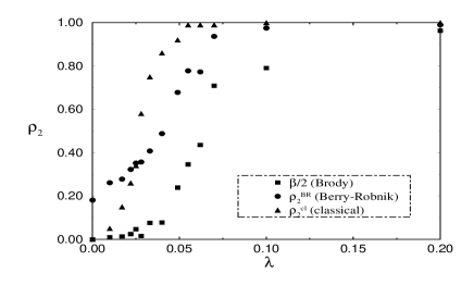
FIG. 5.: Calculated values of $\rho_{2}^{cl}$, $\rho_{2}^{BR}$ and ${\textstyle{1\over 2}}\beta_{Brody}$ as functions of $\lambda$.

The quantum parameter $\rho_{2}^{BR}$ is determined through fitting to the equation (8) and should be compared to the classical measure $\rho_{2}^{cl}$. The results are presented in Fig. 5 and in Table I. In insets of Fig. 2 the fine scale deviations from the Berry-Robnik formula are plotted in terms of the $U(W(S))-U(W^{BR}(S))$ vs. $W(S)$ (full line). We also plot $U(W^{Brody}(S))-U(W^{BR}(S))$ for comparison (dashed line). The transformation $U(W)={\textstyle{2\over\pi}}\arccos{\sqrt{1-W}}$ is used [6] in order to have uniform statistical error over the plot, $\delta U=1/(\pi\sqrt{N})$. The dotted horizontal lines indicate $\pm\delta U$. The Berry-Robnik fit is not statistically significant and the values of the fitting parameters $\rho_{2}^{\rm BR}$ are different from the classical values $\rho_{2}^{\rm cl}$. Why this is so and how the crossover from Brody-like behaviour to Berry-Robnik takes place is discussed in [16]. As one can see at small $S$ (and therefore at small $W(S)$) the agreement with Brody is better than Berry-Robnik, and occasionally, like e.g. at $\lambda=0.055$ and $0.040$, even globally Brody seems to capture the behaviour of our data, although, on the other hand, there are expected deviations at large $S$ (and large $W(S)$) e.g. in the fully chaotic case of Africa billiard ($\lambda=0.2$), where $\beta=1.93$, and Brody asymptotic behaviour at large $S$ is certainly wrong, because its exponent varies $\propto S^{3}$, which is different from GUE in equation (5), $\propto S^{2}$. What we see in this $U$-function representation is consistent with the $T$-function representation in Fig. 3.

In this paper we have presented the numerical computation and statistical analysis of energy spectra of a Hamiltonian system with mixed classical dynamics and without antiunitary symmetry, namely the Aharonov-Bohm cubic conformal plane billiard. We reconfirmed the GUE statistics in the ergodic (fully chaotic) case with approximately 6000 good consecutive energy levels whose accuracy is better than one percent of the mean level spacing. Further, in the KAM regime we have found the fractional power law level repulsion with the exponent varying smoothly from zero to two as the corresponding classical dynamics goes from integrable to ergodic. On the other hand we know that in the ultimate semiclassical limit the Berry-Robnik theory [7, 16] should apply, which does not exhibit level repulsion ($P^{BR}(S=0)=\rho_{1}^{2}\neq 0$). The resolution of this disagreement lies in the fact that the key assumptions of the Berry-Robnik theory are fulfilled only for extremely large sequential quantum numbers or small effective Planck’s constant. Namely, one should require extendedness of the Wigner functions on the whole corresponding classically allowed invariant components of phase space. This is true only if the Heisenberg time, $t_{H}=2\pi\hbar/\langle\Delta E\rangle$ (the time until the discreteness of the spectrum is not yet resolved and the quantum evolution follows the classical one), is larger than the classical ergodic time, $t_{e}$ (the typical time after which classical distributions reach equilibrium steady state on the invariant set). In our case we have typically $t_{e}\gtrsim 10^{4}$ (velocity is one), so the condition $t_{H}>t_{e}$ yields that the sequential number $N$ should be larger than about $10^{8}$. We believe that our present work contributes to the new developements in the wide field of research of quantum chaos, recently reviewed by Weidenmüller et al. [17].

- [1] M. Robnik Lecture Notes in Physics 226, 120 (1986).
- [2] M. V. Berry and M. Robnik J. Phys. A: Math. Gen. 19, 649 (1986).
- [3] M. Robnik J. Phys. A: Math. Gen. 26 1399, 3593 (1992).
- [4] O. Bohigas, M. J. Giannoni, and C. Schmit Phys. Rev. Lett. 226, 120 (1984).
- [5] T. Prosen and M. Robnik J. Phys. A: Math. Gen. 27 8059 (1994).
- [6] T. Prosen and M. Robnik J. Phys. A: Math . Gen. 26, 1105 (1993).
- [7] M. V. Berry and M. Robnik J. Phys. A: Math. Gen. 17 2413 (1984).
- [8] F. Haake Quantum Signatures of Chaos, Berlin: Springer, (1992).
- [9] O. Bohigas, S. Tomsovic, and D. Ullmo Physics Reports, 223, No. 2 , 43-133 (1993).
- [10] J. Dobnikar Spectral statistics in the transition region between integrability and chaos for systems with broken antiunitary symmetry, Diploma thesis, CAMTP and Physics department, FMF, University of Ljubljana, (1996), unpublished.
- [11] M. Robnik Open Systems and Information Dynamics 4 211 (1997).
- [12] M. Robnik J. Phys. A: Math. Gen. 17 1049 (1984).
- [13] T. A. Brody Lett. Nuovo Cimento 7 482 (1973).
- [14] M. V. Berry Proc. Roy. Soc. London A400 229 (1985).
- [15] M. Robnik, J. Dobnikar, A. Rapisarda, T. Prosen, and M. Petkovšek J. Phys. A: Math. Gen., in press.
- [16] M. Robnik and T. Prosen J. Phys. A: Math. Gen. 30 in press (1997).
- [17] T. Guhr, A. Müller-Groeling and H. A. Weidenmüller Random Matrix Theories in Quantum Physics: Common Concepts, MPI Preprint H V27, MPIfK Heidelberg, cond-mat/9707301, July 1997.