Symbolic dynamics analysis of the Lorenz equations

Abstract

Recent progress of symbolic dynamics of one- and especially two-dimensional maps has enabled us to construct symbolic dynamics for systems of ordinary differential equations (ODEs). Numerical study under the guidance of symbolic dynamics is capable to yield global results on chaotic and periodic regimes in systems of dissipative ODEs which cannot be obtained neither by purely analytical means nor by numerical work alone. By constructing symbolic dynamics of 1D and 2D maps from the Poincaré sections all unstable periodic orbits up to a given length at a fixed parameter set may be located and all stable periodic orbits up to a given length may be found in a wide parameter range. This knowledge, in turn, tells much about the nature of the chaotic limits. Applied to the Lorenz equations, this approach has led to a nomenclature, i.e., absolute periods and symbolic names, of stable and unstable periodic orbits for an autonomous system. Symmetry breakings and restorations as well as coexistence of different regimes are also analyzed by using symbolic dynamics.

I. INTRODUCTION

Many interesting nonlinear models in physical sciences and engineering are given by systems of ODEs. When studying these systems it is desirable to have a global understanding of the bifurcation and chaos “spectrum”: the systematics of periodic orbits, stable as well as unstable ones at fixed and varying parameters, the type of chaotic attractors which usually occur as limits of sequences of periodic regimes, etc. However, this is by far not a simple job to accomplish neither by purely analytical means nor by numerical work alone. In analytical aspect, just recollect the long-standing problem of the number of limit cycles in planar systems of ODEs. As chaotic behavior may appear only in systems of more than three autonomous ODEs, it naturally leads to problems much more formidable than counting the number of limit cycles in planar systems. As numerical study is concerned, one can never be confident that all stable periodic orbits up to a certain length have been found in a given parameter range or no short unstable orbits in a chaotic attractor have been missed at a fixed parameter set, not to mention that it is extremely difficult to draw global conclusions from numerical data alone.

On the other hand, a properly constructed symbolic dynamics, being a coarse-grained description, provides a powerful tool to capture global, topological aspects of the dynamics. This has been convincingly shown in the development of symbolic dynamics of one-dimensional (1D) maps, see, e.g., [1, 2, 3, 4, 5]. Since it is well known from numerical observations that chaotic attractors of many higher-dimensional dissipative systems with one positive Lyapunov exponent reveal 1D-like structure in some Poincaré sections, it has been suggested to associate the systematics of numerically found periodic orbits in ODEs with symbolic dynamics of 1D maps [6]. While this approach has had some success (see, e.g., Chapter 5 of [4]), many new questions arose from the case studies. For example,
1. The number of short stable periodic orbits found in ODEs is usually less than that allowed by the admissibility conditions of the corresponding 1D symbolic dynamics. Within the 1D framework it is hard to tell whether a missing period was caused by insufficient numerical search or was forbidden by the dynamics.

2. In the Poincaré sections of ODEs, at a closer examination, the attractors often reveal two-dimensional features such as layers and folds. One has to explain the success of 1D description which sometimes even turns out much better than expected. At the same time, the limitation of 1D approach has to be analyzed as the Poincaré maps are actually two-dimensional.

3. Early efforts were more or less concentrated on stable orbits, while unstable periods play a fundamental role in organizing chaotic motion. One has to develop symbolic dynamics for ODEs which would be capable to treat stable and unstable periodic orbits alike, to indicate the structure of some, though not all, chaotic orbits at a given parameter set.

The elucidation of these problems has to await a significant progress of symbolic dynamics of 2D maps. Now the time is ripe for an in depth symbolic dynamics analysis of a few typical ODEs. This kind of analysis has been carried out on several non-autonomous systems [7, 8, 9], where the stroboscopic sampling method [10] greatly simplifies the calculation of Poincaré maps. In this paper we consider an autonomous system, namely, the Lorenz model, in which one of the first chaotic attractor was discovered [11].

The Lorenz model consists of three equations

$${\dot{x}}=\sigma(y-x),\quad{\dot{y}}=rx-y-xy,\quad{\dot{z}}=xy-bx.$$ (1)

It is known that several models of hydrodynamical, mechanical, dynamo and laser problems may be reduced to this set of ODEs. The system (1) contains three parameters $r$, $\sigma$ and $b$, representing respectively the Rayleigh number, the Prandtl number and a geometric ratio. We will study the system in a wide $r$-range at fixed $\sigma=10$ and $b=8/3$.

We put together a few known facts on Eq. 1 to fix the notations. For detailed derivations one may refer to the book [12] by C. Sparrow. For $0<r<1$ the origin $(0,0,0)$ is a globally stable fixed point. It loses stability at $r=1$. A 1D unstable manifold and a 2D stable manifold ${\cal W}^{s}$ come out from the unstable origin. The intersection of the 2D ${\cal W}^{s}$ with the Poincaré section will determine a demarcation line in the partition of the 2D phase plane of the Poincaré map. For $r>1$ there appears a pair of fixed points

$$C_{\pm}=(\pm\sqrt{b(r-1)},\pm\sqrt{b(r-1)},r-1).$$

These two fixed points remain stable until $r$ reaches 24.74. Although their eigenvalues undergo some qualitative changes at $r=1.345617$ and a strange invariant set (not an attractor yet) comes into life at $r=13.926$, here we are not interested in all this. It is at $r=24.74$ a sub-critical Hopf bifurcation takes place and chaotic regimes commence. Our $r$-range extends from 28 to very big values, e.g., 10000, as nothing qualitatively new appears at, say, $r>350$.

Before undertaking the symbolic dynamics analysis we summarize briefly what has been done on the Lorenz system from the viewpoint of symbolic dynamics. Guckenheimer and Williams introduced the geometric Lorenz model [13] for the vicinity of $r=28$ which leads to symbolic dynamics on two letters, proving the existence of chaos in the geometric model. However, as Smale [14] pointed out it remains an unsolved problem as whether the geometric Lorenz model means to the real Lorenz system. Though not using symbolic dynamics at all, the paper by Tomita and Tsuda [15] studying the Lorenz equations at a different set of parameters $\sigma=16$ and $b=4$ is worth mentioning. They noticed that the quasi-1D chaotic attractor in the $z=r-1$ Poincaré section outlined by the upward intersections of the trajectories may be directly parameterized by the $x$ coordinates. A 1D map was devised in [15] to numerically mimic the global bifurcation structure of the Lorenz model. C. Sparrow [12] used two symbols $x$ and $y$ to encode orbits without explicitly constructing symbolic dynamics. In Appendix J of [12] Sparrow described a family of 1D maps as “an obvious choice if we wish to try and model the behavior of the Lorenz equations in the parameter range $\sigma=10$, $b=8/3$ and $r>24.06$”. In what follows we will call this family the Lorenz-Sparrow map. Refs. [15] and [12] have been instrumental for the present study. In fact, the 1D maps to be obtained from the 2D upward Poincaré maps of the Lorenz equations after some manipulations belong precisely to the family suggested by Sparrow. In [16] the systematics of stable periodic orbits in the Lorenz equations was compared with that of a 1D anti-symmetric cubic map. The choice of an anti-symmetric map was dictated by the invariance of the Lorenz equations under the discrete transformation

$$x\rightarrow-x,\quad y\rightarrow-y,\quad{\rm and}\quad z\rightarrow z.$$ (2)

Indeed, most of the periods known to [16] are ordered in a “cubic” way. However, many short periods present in the 1D map have not been found in the Lorenz equations. It was realized in [17] that a cubic map with a discontinuity in the center may better reflect the ODEs and many of the missing periods are excluded by the 2D nature of the Poincaré map. Instead of devising model maps for comparison one should generate all related 1D or 2D maps directly from the Lorenz equations and construct the corresponding symbolic dynamics. This makes the main body of the present paper.

Figure 1: An upward Poincaré section at $r=118.15$. The dashed curve is one of the forward contracting foliations and the diamond a tangent point between the FCF and BCF.

For physicists symbolic dynamics is nothing but a coarse-grained description of the dynamics. The success of symbolic dynamics depends on how the coarse-graining is performed, i.e., on the partition of the phase space. From a practical point of view we can put forward the following requirements for a good partition. 1. It should assign a unique name to each unstable periodic orbit in the system; 2. An ordering rule of all symbolic sequences should be defined; 3. Admissibility conditions as whether a given symbolic sequence is allowed by the dynamics should be formulated; 4. Based on the admissibility conditions and ordering rule one should be able to generate and locate all periodic orbits, stable and unstable, up to a given length. Symbolic dynamics of 1D maps has been well understood [1, 2, 3, 4, 5]. Symbolic dynamics of 2D maps has been studies in [18, 19, 20, 21, 22, 23, 24, 25, 26, 27]. We will explain the main idea and technique in the context of the Lorenz equations.

A few words on the research strategy may be in order. We will first calculate the Poincaré maps in suitably chosen sections. If necessary some forward contracting foliations (FCFs, to be explained later) are superimposed on the Poincaré map, the attractor being part of the backward contracting foliations (BCFs). Then a one-parameter parameterization is introduced for the quasi-1D attractor. For our choice of the Poincaré sections the parameterization is simply realized by the $x$ coordinates of the points. In terms of these $\{x_{i}\}$ a first return map $x_{n}\mapsto x_{n+1}$ is constructed. Using the specific property of first return maps that the set $\{x_{i}\}$ remains the same before and after the mapping, some parts of $\{x_{i}\}$ may be safely shifted and swapped to yield a new map $x_{n}^{\prime}\mapsto x_{n+1}^{\prime}$, which precisely belongs to the family of Lorenz-Sparrow map. In so doing, all 2D features (layers, folds, etc.) are kept. However, one can always start from the symbolic dynamics of the 1D Lorenz-Sparrow map to generate a list of allowed periods and then check them against the admissibility conditions of the 2D symbolic dynamics. Using the ordering of symbolic sequences all allowed periods may be located easily. What said applies to unstable periodic orbits at fixed parameter set. The same method can be adapted to treat stable periods either by superimposing the orbital points on a near-by chaotic attractor or by keeping a sufficient number of transient points.

Figure 2: The first return map $x_{n}\mapsto x_{n+1}$ constructed from Fig. 1 by using the $x$ coordinates.

II. CONSTRUCTION OF POINCARÉ AND
RETURN MAPS

The Poincaré map in the $z=r-1$ plane captures most of the interesting dynamics as it contains both fixed points $C_{\pm}$. The $z$-axis is contained in the stable manifold ${\cal W}^{s}$ of the origin $(0,0,0)$. All orbits reaching the $z$-axis will be attracted to the origin , thus most of the homoclinic behavior may be tracked in this plane. In principle, either downward or upward intersections of trajectories with the $z=r-1$ plane may be used to generate the Poincaré map. However, upward intersections with $dz/dt>0$ have the practical merit to yield 1D-like objects which may be parameterized by simply using the $x$ coordinates.

Fig. 1 shows a Poincaré section at $r=118.15$. The dashed curves and diamonds represent one of the FCFs and its tangent points with the BCF. These will be used later in Sec. V. The 1D-like structure of the attractor is apparent. Only the thickening in some part of the attractor hints on 2D structures. Ignoring the thickening for the time being, the 1D attractor may be parameterized by the $x$ coordinates only. Collecting successive $x_{i}$, we construct a first return map $x_{n}\mapsto x_{n+1}$ as shown in Fig. 2. It consists of four symmetrically located pieces with gaps on the mapping interval. For a first return map a gap belonging to both $\{x_{n}\}$ and $\{x_{n+1}\}$ plays no role in the dynamics. If necessary, we can use this specificity of return maps to squeeze some gaps in $x$. Furthermore, we can interchange the left subinterval with the right one by defining, e.g.,

$$x^{\prime}=x-36\quad{\rm for}\quad x>0;\qquad x^{\prime}=x+36\quad{\rm for}\quad x<0.$$ (3)

The precise value of the numerical constant is not essential; it may be estimated from the upper bound of $\{|x_{i}|\}$ and is so chosen as to make the final figure look nicer. The swapped first return map, as we call it, is shown in Fig. 3. The corresponding tangent points between FCF and BCF (the diamonds) are also drawn on these return maps for later use.

Figure 3: The swapped return map $x_{n}^{\prime}\mapsto x_{n+1}^{\prime}$ constructed from Fig. 2. The gaps may be further squeezed, see text.

Figure 4: Upward Poincaré maps at 9 different $r$-values.

Figure 5: Swapped first return maps obtained from the Poincaré maps shown in Fig. 4.

It is crucial that the parameterization and swapping do keep the 2D features present in the Poincaré map. This is important when it comes to take into account the 2D nature of the Poincaré maps.

In Fig. 4 Poincaré maps at 9 different values from $r=28$ to 203 are shown. The corresponding swapped return maps are shown in Fig. 5. Generally speaking, as $r$ varies from small to greater values, these maps undergo transitions from 1D-like to 2D-like, and then to 1D-like again. Even in the 2D-like range the 1D backbones still dominate. This partly explains our early success [16, 17] in applying purely 1D symbolic dynamics to the Lorenz model. We will learn how to judge this success later on. Some qualitative changes at varying $r$ will be discussed in Sec. III. We note also that the return map at $r=28$ complies with what follows from the geometric Lorenz model. The symbolic dynamics of this Lorenz-like map has been completely constructed [28].

III. SYMBOLIC DYNAMICS OF THE
1D LORENZ-SPARROW MAP

All the return maps shown in Fig. 5 fit into the family of Lorenz-Sparrow map. Therefore, we take a general map from the family and construct the symbolic dynamics. There is no need to have analytical expression for the map. Suffice it to define a map by the shape shown in Fig. 6. This map has four monotone branches, defined on four subintervals labeled by the letters $M$, $L$, $N$, and $R$, respectively. We will also use these same letters to denote the monotone branches themselves, although we do not have an expression for the mapping function $f(x)$. Among these branches $R$ and $L$ are increasing; we say $R$ and $L$ have an even or $+$ parity. The decreasing branches $M$ and $N$ have odd or $-$ parity. Between the monotone branches there are “turning points” (“critical points”) $D$ and $C$ as well as “breaking point” $B$, where a discontinuity is present. Any numerical trajectory $x_{1}x_{2}\cdots x_{i}\cdots$ in this map corresponds to a symbolic sequence

$$\Sigma=\sigma_{1}\sigma_{2}\cdots\sigma_{i}\cdots,$$

where $\sigma_{i}\in\{M,L,N,R,C,D,B\}$, depending on where the point $x_{i}$ falls in.

Ordering and admissibility of symbolic sequences

All symbolic sequences made of these letters may be ordered in the following way. First, there is a natural order

$$N<C<R<B<L<D<M.$$ (4)

Next, if two symbolic sequences $\Sigma_{1}$ and $\Sigma_{2}$ have a common leading string $\Sigma^{\ast}$, i.e.,

$$\Sigma_{1}=\Sigma^{\ast}\sigma\cdots,\quad\Sigma_{2}=\Sigma^{\ast}\tau\cdots,$$

where $\sigma\neq\tau$. Since $\sigma$ and $\tau$ are different, they must have ordered according to (4). The ordering rule is: if $\Sigma$ is even, i.e., it contains an even number of $N$ and $M$, the order of $\Sigma_{1}$ and $\Sigma_{2}$ is given by that of $\sigma$ and $\tau$; if $\Sigma^{\ast}$ is odd, the order is the opposite to that of $\sigma$ and $\tau$. The ordering rule may be put in the following form:

$$EN\cdots < EC\cdots<ER\cdots<EB\cdots$$

$$< EL\cdots<ED\cdots<EM\cdots,$$

$$ON\cdots > OC\cdots>OR\cdots>OB\cdots$$

$$> OL\cdots>OD\cdots>OM\cdots,$$

where $E$ ($O$) represents a finite string of $M$, $L$, $N$, and $R$ containing an even (odd) number of letters $M$ and $N$. We call $E$ and $O$ even and odd string, respectively.

Figure 6: A generic Lorenz-Sparrow map. The symbols $M$, $L$, $R$, and $N$ label the monotone branches as well as the subintervals. $C$, $D$ and $B$ are turning or breaking points. For $H$ and $\overline{H}$ see text.

In order to incorporate the discrete symmetry, we define a transformation ${\cal T}$ of symbols:

$${\cal T}=\{M\leftrightarrow N,L\leftrightarrow R,C\leftrightarrow D\},$$ (6)

keeping $B$ unchanged. Sometimes we distinguish the left and right limit of $B$, then we add $B_{-}\leftrightarrow B_{+}$. We often denote ${\cal T}\Sigma$ by $\overline{\Sigma}$ and say $\Sigma$ and $\overline{\Sigma}$ are mirror images to each other.

Symbolic sequences that start from the next iterate of the turning or breaking points play a key role in symbolic dynamics. They are called kneading sequences [3]. Naming a symbolic sequence by the initial number which corresponds to its first symbol, we have two kneading sequences from the turning points:

$$K=f(C),\qquad\overline{K}=f(D).$$

Being mirror images to each other, we take $K$ as the independent one.

For first return maps the rightmost point in $\{x_{i}\}$ equals the highest point after the mapping. Therefore, $f(B_{-})=H$ and $f(B_{+})=\overline{H}$, see Fig. 6. We take $H$ as another kneading sequence. Note that $B_{-}$ and $B_{+}$ are not necessarily the left and right limit of the breaking point; a finite gap may exist in between. This is associated with the flexibility of choosing the shift constant, e.g., the number 36 in (3). Since a kneading sequence starts from the first iterate of a turning or breaking point, we have

$$C_{-} = NK,\quad C+=RK,\quad B_{-}=RH,$$

$$B_{+} = L\overline{H},\quad D_{-}=L\overline{K},\quad D_{+}=M\overline{K}.$$

A 1D map with multiple critical points is best parameterized by its kneading sequences. The dynamical behavior of the Lorenz-Sparrow map is entirely determined by a kneading pair $(K,H)$. Given a kneading pair $(K,H)$, not all symbolic sequences are allowed in the dynamics. In order to formulate the admissibility conditions we need a new notion. Take a symbolic sequence $\Sigma$ and inspect its symbols one by one. Whenever a letter $M$ is encountered, we collect the subsequent sequence that follows this $M$. The set of all such sequences is denoted by ${\cal M}(\Sigma)$ and is called a $M$-shift set of $\Sigma$. Similarly, we define ${\cal L}(\Sigma)$, ${\cal R}(\Sigma)$ and ${\cal N}(\Sigma)$.

The admissibility conditions, based on the ordering rule (Ordering and admissibility of symbolic sequences), follow from (Ordering and admissibility of symbolic sequences):

$$\overline{H} \leq N{\cal N}(\Sigma)\leq NK,\quad K\leq{\cal R}(\Sigma)\leq H,$$

$$\overline{H} \leq {\cal L}(\Sigma)\leq\overline{K},\quad M\overline{K}\leq M{\cal M}(\Sigma)\leq H.$$

Here in the two middle relations we have canceled the leading $R$ or $L$.

The twofold meaning of the admissibility conditions should be emphasized. On one hand, for a given kneading pair these conditions select those symbolic sequences which may occur in the dynamics. On the other hand, a kneading pair $(K,H)$, being symbolic sequences themselves, must also satisfy conditions (Ordering and admissibility of symbolic sequences) with $\Sigma$ replaced by $K$ and $H$. Such $(K,H)$ is called a compatible kneading pair. The first meaning concerns admissible sequences in the phase space at a fixed parameter set while the second deals with compatible kneading pairs in the parameter space. In accordance with these two aspects there are two pieces of work to be done. First, generate all compatible kneading pairs up to a given length. This is treated in Appendix A. Second, generate all admissible symbolic sequences up to a certain length for a given kneading pair $(K,H)$. The procedure is described in Appendix B.

Metric representation of symbolic sequences

It is convenient to introduce a metric representation of symbolic sequences by associating a real number $0\leq\alpha(\Sigma)\leq 1$ to each sequence $\Sigma$. To do so let us look at the piecewise linear map shown in Fig. 7. It is an analog of the surjective tent map in the sense that all symbolic sequences made of the four letters $M$, $L$, $R$, and $N$ are allowed. It is obvious that the maximal sequence is $(MN)^{\infty}$ while the minimal one being $(NM)^{\infty}$. For this map one may further write

$$C_{-}=N(NM)^{\infty},C+=R(NM)^{\infty},B_{-}=R(MN)^{\infty},$$

$$B_{+}=L(NM)^{\infty},D_{-}=L(MN)^{\infty},D_{+}=M(MN)^{\infty}.$$

Figure 7: A piecewise linear map used to introduce metric representation for the Lorenz-Sparrow map.

To introduce the metric representation we first use $\epsilon=1$ to mark the even parity of $L$ and $R$, and $\epsilon=-1$ to mark the odd parity of $M$ and $N$. Next, the number $\alpha(\Sigma)$ is defined for a sequence $\Sigma=s_{1}s_{2}\cdots s_{i}\cdots$ as

$$\alpha=\sum_{i=1}^{\infty}\mu_{i}4^{-i},$$ (9)

where

$$\mu_{i}=\cases{0\cr 1\cr 2\cr 3\cr}\quad{\rm for}\quad s_{i}=\cases{N\cr R\cr L\cr M\cr}\quad{\rm if}\quad\epsilon_{1}\epsilon_{2}\cdots\epsilon_{i-1}=1,$$

or,

$$\mu_{i}=\cases{3\cr 2\cr 1\cr 0\cr}\quad{\rm for}\quad s_{i}=\cases{N\cr R\cr L\cr M\cr}\quad{\rm if}\quad\epsilon_{1}\epsilon_{2}\cdots\epsilon_{i-1}=-1.$$

It is easy to check that

$$\alpha((NM)^{\infty}) = 0,\quad\alpha(C_{\pm})=1/4,\quad\alpha(B_{\pm})=1/2,$$

$$\alpha(D_{\pm}) = 3/4,\quad\alpha((MN)^{\infty})=1.$$

The following relations hold for any symbolic sequence $\Sigma$:

$$\alpha(\overline{\Sigma})=1-\alpha(\Sigma),\quad\alpha(L\Sigma) = (2+\alpha(\Sigma))/4,$$

$$\alpha(R\Sigma) = (1+\alpha(\Sigma))/4.$$

One may also formulate the admissibility conditions in terms of the metric representations.

One-parameter limits of the Lorenz-Sparrow map

The family of the Lorenz-Sparrow map includes some limiting cases.
1. The $N$ branch may disappear, and the minimal point of the $R$ branch moves to the left end of the interval. This may be described as

$$C=\overline{H}=RK,\quad{\rm or}\quad H=L\overline{K}.$$ (11)

It defines the only kneading sequence $K$ from the next iterate of $C$.

2. The minimum at $C$ may rise above the horizontal axis, as it is evident in Fig. 5 at $r=203$. The second iterate of either the left or right subinterval then retains in the same subinterval. Consequently, the two kneading sequences are no longer independent and they are bound by the relation

$$K=L\overline{H},\quad{\rm or}\quad\overline{K}=RH.$$ (12)

Both one-parameter limits appear in the Lorenz equations as we shall see in the next section.

IV. 1D SYMBOLIC DYNAMICS OF THE
LORENZ EQUATIONS

Now we are well prepared to carry out a 1D symbolic dynamics analysis of the Lorenz equations using the swapped return maps shown in Fig. 5. We take $r=118.15$ as an working example. The rightmost point in $\{x_{i}\}$ and the minimum at $C$ determine the two kneading sequences:

$$H = MRLNRLRLRLRLNRL\cdots,$$

$$K = RLRLRLRRLRLRLRR\cdots.$$

Indeed, they satisfy (Ordering and admissibility of symbolic sequences) and form a compatible kneading pair. Using the propositions formulated in Appendix B, all admissible periodic sequences up to period 6 are generated. They are $LC$, $LNLR$, $LNLRLC$, $RMRLR$, $RMLNLC$, $RMLN$, $RLLC$, $RLLNLC$, $RLRMLC$, and $RLRLLC$. Here the letter $C$ is used to denote both $N$ and $R$. Therefore, there are altogether 17 unstable periodic orbits with period equal or less than 6. Relying on the ordering of symbolic sequences and using a bisection method, these unstable periodic orbits may be quickly located in the phase plane.

It should be emphasized that we are dealing with unstable periodic orbits at a fixed parameter set. There is no such thing as superstable periodic sequence or periodic window which would appear when one considers kneading sequences with varying parameters. Consequently, the existence of $LN$ and $LR$ does not necessarily imply the existence of $LC$.

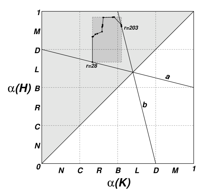
Figure 8: The $\alpha(H)$ versus $\alpha(K)$ plane shows kneading pairs (solid circles) corresponding to the Lorenz equations from $r=28$ to 203. Only the upper left triangular region is accessible for compatible pairs in the Loren-Sparrow map. The two straight lines a and b represent the two one-parameter limits of the Lorenz-Sparrow map.

Similar analysis may be carried out for other $r$. In Table 1 we collect some kneading sequences at different $r$-values. Their corresponding metric representations are also included. We first note that they do satisfy the admissibility conditions (Ordering and admissibility of symbolic sequences), i.e., $K$ and $H$ at each $r$ make a compatible kneading pair. An instructive way of presenting the data consists in drawing the plane of metric representation for both $\alpha(K)$ and $\alpha(H)$, see Fig. 8. The compatibility conditions require, in particular, $K\leq H$, therefore only the upper left triangular region is accessible.

Table 1: Kneading pairs $(K,H)$ and their metric representations at different $r$-values.

$r$	$K$	$\alpha(K)$	$H$	$\alpha(H)$
203.0	LNLRLRLRLRLRLRL	0.525000	MRLRLRLRLRLRLRL	0.900000
201.0	LNLRLRLRMRLRLRM	0.524995	MRLRLRLNLRLRLNL	0.900018
199.04	LNLRLRMRLRLNLRL	0.524927	MRLRLNLRLRMRLRL	0.900293
198.50	LNLRMRMRLRMRMRL	0.523901	MRLNLNLRLNLNLRL	0.904396
197.70	LNLRMRLRLRLNLRL	0.523828	MRLNLRLRLRMRLRL	0.904688
197.65	LNLRMRLRLNLRLRM	0.523827	MRLNLRLRMRLRLNL	0.904692
197.58	LNLRMRRMRMRLRMR	0.523796	MRRMRMRLNLNLRLR	0.908110
196.20	LNLLNLRLNLRLRLN	0.523042	MRRLRLRLRLRLNLR	0.912500
191.0	RMRLNLNLLRLRLRM	0.476096	MNRLRLRMRLRMLNL	0.962518
181.8	RMRLLNLRRMRLLNL	0.475410	MNRLRLRLRLRLRLN	0.962500
166.2	RMLNRMLNRMLNRML	0.466667	MNRLNRMRLRLLNRM	0.961450
139.4	RLRMRLRRLLNLRRL	0.404699	MNRRLLNRMLRRLLR	0.959505
136.5	RLRMLRRLRMRLLRL	0.403954	MNRRLLNLRRLRMLR	0.959498
125.0	RLRLLNLRLRRLRLL	0.400488	MRRLRMLRLRRLRLL	0.912256
120.0	RLRLRLRLRLRLRML	0.400000	MRRMLRLRLRLRLRR	0.908594
118.15	RLRLRLRRLRLRLRR	0.399988	MRLNRLRLRLRLNRL	0.903906
117.7	RLRLRLNRLLRLRLR	0.399938	MRLRRLRLRLNRLLR	0.900781
114.02	RLRLRRLRLRRLRLR	0.399804	MRLRLNRLRLRRLRL	0.900244
107.7	RLRRLLRRLRRLLRR	0.397058	MRLLRRLLRLLNRLR	0.897058
104.2	RLRRLRLRRLRRLRL	0.396872	MRLLRLLRLRRLLNR	0.896826
101.5	RLRRLRRLRRLRLNR	0.396825	MLNRMLRLLRLLRLL	0.866598
99.0	RLNRLRRLRRLRRLR	0.384425	MLNRLRRLNRLRRLN	0.865572
93.4	RRMLLNRRMLLNRLL	0.365079	MLRRLLRRRMLRLLR	0.852944
83.5	RRLLRRRLLRRRLLR	0.352884	MLRLLRLRRRLLLRR	0.849233
71.7	RRLRRRLRRRLRRLR	0.349020	MLLRLRRLLRRLLLR	0.837546
69.9	RRRMLLLNRRRMLLR	0.341176	MLLRLRLLLRLLRLR	0.837485
69.65	RRRLLLLNRRRMLLR	0.338511	MLLRLLNRRLRRLLR	0.837363
65.0	RRRLLRRRRLLRLLR	0.338217	MLLLRRRLRRRLLRL	0.834620
62.2	RRRLRLRRRLRRRRM	0.337485	MLLLRRLLLLRLRLL	0.834554
59.4	RRRLRRRRLRRRLLL	0.337243	MLLLRLLRLRRLRLL	0.834326
55.9	RRRRLLRRRRLRLLR	0.334554	MLLLLRRLRRLLLLR	0.833643
52.6	RRRRLRRRRRLLRRR	0.334310	MLLLLRLLLLRRRRR	0.833578
50.5	RRRRRLLRRRLRLRL	0.333639	MLLLLLRRLLRRLRR	0.833410
48.3	RRRRRLRRRRRLLLL	0.333578	MLLLLLRLLLLRLLR	0.833394
48.05	RRRRRRLLLLLRLLL	0.333415	MLLLLLRLLLLLLLR	0.833394
46.0	RRRRRRLRLRRRRLL	0.333398	MLLLLLLRLRLLLLN	0.833350
44.0	RRRRRRRLRLLLLLL	0.333350	MLLLLLLLRLRRRRR	0.833337
36.0	RRRRRRRRRRRRRLR	0.333333	MLLLLLLLLLLLLLR	0.833333
28.0	RRRRRRRRRRRRRRR	0.333333	LLLLLLLLLLLLLLL	0.666667

As we have indicated at the end of the last section, the Lorenz-Sparrow map has two one-parameter limits. The first limit (11) takes place somewhere at $r<36$, maybe around $r<30.1$, as estimated by Sparrow [12] in a different context. In Table 1 there is only one kneading pair $K=R^{\infty}$ and $H=L^{\infty}$ satisfying $H=L\overline{K}$. In terms of the metric representations the condition (11) defines a straight line (line a in Fig. 8)

$$\alpha(H)=(3-\alpha(K))/4.$$

(We have used (Metric representation of symbolic sequences)). The point $r=28$ drops down to this line almost vertically from the $r=36$ point. This is the region where “fully developed chaos” has been observed in the Lorenz model and perhaps it outlines the region where the geometric Lorenz model may apply.

The other limit (12) happens at $r>197.6$. In Table 1 all 6 kneading pairs in this range satisfy $K=L\overline{H}$. They fall on another straight line (line b in Fig. 8)

$$\alpha(K)=(3-\alpha(H))/4,$$

but can hardly be resolved. The value $r=197.6$ manifests itself as the point where the attractor no longer crosses the horizontal axis. In the 2D Poincaré map this is where the chaotic attractor stops to cross the stable manifold ${\cal W}^{s}$ of the origin. The kneading pair at $r=203$ is very close to a limiting pair $K=LN(LR)^{\infty}$ with a precise value $\alpha=21/40=0.525$ and $H=M(RL)^{\infty}$ with exact $\alpha=0.9$.

For any kneading pair in Table 1 one can generate all admissible periods up to length 6 inclusively. For example, at $r=125$ although the swapped return map shown in Fig. 5 exhibits some 2D feature as throwing a few points off the 1D attractor, the 1D Lorenz-Sparrow map still works well. Besides the 17 orbits listed above for $r=118.15$, five new periods appear: $LLN$, $LNLRMR$, $LNLLC$, and $RMRLN$. All these 22 unstable periodic orbits have been located with high precision in the Lorenz equations. Moreover, if we confine ourselves to short periods not exceeding period 6, then from $r=28$ to 59.40 there are only symbolic sequences made of the two letters $R$ and $L$. In particular, From $r=28$ to 50.50 there exist the same 12 unstable periods: $LR$, $RLR$, $RLLR$, $RRLR$, $RLRLR$, $RRLLR$, $RRRLR$, $RLRLLR$, $RRLLLR$, $RRLRLR$, $RRRLLR$, and $RRRRLR$. This may partly explain the success of the geometric Lorenz model leading to a symbolic dynamics on two letters. On the other hand, when $r$ gets larger, e.g., $r=136.5$, many periodic orbits “admissible” to the 1D Lorenz-Sparrow map, cannot be found in the original Lorenz equations. This can only be analyzed by invoking 2D symbolic dynamics of the Poincaré map.

V. SYMBOLIC DYNAMICS OF THE
2D POINCARÉ MAPS

Essentials of 2D symbolic dynamics

The extension of symbolic dynamics from 1D to 2D maps is by no means trivial. First of all, the 2D phase plane has to be partitioned in such a way as to meet the requirements of a “good” partition that we put forward in Sec. I. Next, as 2D maps are in general invertible, a numerical orbit is encoded into a bi-infinite symbolic sequence

$$\cdots s_{\overline{m}}\cdots s_{\overline{2}}s_{\overline{1}}\bullet s_{1}s_{2}\cdots s_{n}\cdots,$$

where a heavy dot $\bullet$ denotes the “present” and one iteration forward or backward corresponds to a left or right shift of the present dot. The half-sequence $\bullet s_{1}s_{2}\cdots s_{n}\cdots$ is called a forward symbolic sequence and $\cdots s_{\overline{m}}\cdots s_{\overline{2}}s_{\overline{1}}\bullet$ a backward symbolic sequence. One should assign symbols to both forward and backward sequences in a consistent way by partitioning the phase plane properly. In the context of the Hénon map Grassberger and Kantz [29] proposed to draw the partition line through tangent points between the stable and unstable manifolds of the unstable fixed point in the attractor. Since pre-images and images of a tangent point are also tangent points, it was suggested to take “primary” tangencies where the sum of curvatures of the two manifolds is minimal [20].

A natural generalization of the Grassberger-Kantz idea is to use tangencies between forward contracting foliations (FCFs) and backward contracting foliations (BCFs) of the dynamics to determine the partition line [24]. Points on one and the same FCF approach each other with the highest speed under forward iterations of the map. Therefore, one may introduce an equivalence relation: points $p_{1}$ and $p_{2}$ belong to the same FCF if they eventually approach the same destination under forward iterations of the map:

$$p_{1}\sim p_{2}\quad{\rm if}\quad\displaystyle\lim_{n\rightarrow\infty}|f^{n}(p_{1})-f^{n}(p_{2})|=0.$$

The collection of all FCFs forms a forward contracting manifold of the dynamics. Points in one and the same FCF have the same future.

Likewise, points on one and the same BCF approach each other with the highest speed under backward iterations of the map. One introduces an equivalence relation: points $p_{1}$ and $p_{2}$ belong to the same BCF if they eventually approach the same destination under backward iterations of the map:

$$p_{1}\sim p_{2}\quad{\rm if}\quad\displaystyle\lim_{n\rightarrow\infty}|f^{-n}(p_{1})-f^{-n}(p_{2})|=0.$$

The collection of all BCFs forms the backward contracting manifold of the dynamics. Points in one and the same BCF have the same history. When the phase space is partitioned properly, points in a FCF acquire the same forward symbolic sequence while points in a BCF acquire the same backward symbolic sequence. this has been shown analytically for the Lozi map [24] and Tél map [25]. There has been good numerical evidence for the Hénon map [19, 20, 26, 27]. We mention in passing that the forward contracting and backward contracting manifolds contain the stable and unstable manifolds of fixed and periodic points as invariant manifolds.

Figure 9: An upward Poincaré section at $r=136.5$ showing the chaotic attractor, a few FCFs (dashed lines), and segments of the partition lines for forward symbolic sequences (dotted lines).

The generalization to use FCFs and BCFs is necessary at least for the following reasons. 1. It is not restricted to the attractor only. The attractor may experience abrupt changes, but the FCF and BCF change smoothly with parameter. This is a fact unproven but supported by much numerical evidence. 2. A good symbolic dynamics assigns unique symbolic names to all unstable orbits, not only those located in the attractor. One needs in partition lines outside the attractor. 3. Transient processes also take place outside the attractor. They are part of the dynamics and should be covered by the same symbolic dynamics.

In practice, contours of BCFs and especially FCFs are not difficult to calculate from the dynamics. This has been shown for BCFs by J. M. Greene [30] and for FCFs by Gu [31]. Once a mesh of BCFs and FCFs are drawn in the phase plane, FCFs may be ordered along some BCF and vice versa. No ambiguity in the ordering occurs as long as no tangency between the two foliations is encountered. A tangency signals that one should change to a symbol of a different parity after crossing a tangency. A tangency in a 2D map plays a role similar to a kneading sequence in a 1D map in the sense that it prunes away some inadmissible sequences. As there are infinitely many tangencies between the FCFs and BCFs, one may say that there is an infinite number of kneading sequences in a 2D map even at a fixed parameter set. However, as one deals with symbolic sequences of finite length only a finite number of tangencies will matter.

Partitioning of the Poincaré section

Lorenz equations at $r=136.5$ provide a typical situation where 2D symbolic dynamics must be invoked. Figure 9 shows an upward $z=r-1$ Poincaré section of the chaotic attractor. The dashed lines indicate the contour of the FCFs. The two symmetrically located families of FCFs are demarcated by the intersection of the stable manifold ${\cal W}^{s}$ of the $(0,0,0)$ fixed point with the $z=r-1$ plane. The actual intersection located between the dense dashed lines is not shown. The BCFs are not shown either except the attractor itself which is a part of the BCFs.

The 1D symbolic dynamics analysis performed in Sec. IV deals with forward symbolic sequences only. However, the partition of the 1D interval shown e.g., in Fig. 3, may be traced back to the 2D Poincaré section to indicate the partition for assigning symbols to the forward symbolic sequences. Two segments of the partition lines are shown in Fig. 9 as dotted lines. The labels $\bullet C$ and $\bullet D$ correspond to $C$ and $D$ in the Lorenz-Sparrow map, see Fig. 3. The ordering rule (Ordering and admissibility of symbolic sequences) should now be understood as:

$$\bullet EN\cdots < \bullet EC\cdots<\bullet ER\cdots<\bullet EB\cdots$$

$$< \bullet EL\cdots<\bullet ED\cdots<\bullet EM\cdots,$$

$$\bullet ON\cdots > \bullet OC\cdots>\bullet OR\cdots>\bullet OB\cdots$$

$$> \bullet OL\cdots>\bullet OD\cdots>\bullet OM\cdots,$$

with $E$ and $O$ being even and odd strings of $M$, $L$, $R$, and $N$. In fact, from Fig. 3 one could only determine the intersection point of the partition line with the 1D-like attractor. To determine the partition line in a larger region of the phase plane one has to locate more tangencies between the FCFs and the BCFs. However, it is more convenient to use another set of tangent points to determine the partition line for backward symbolic sequences. To this end 6 tangent points and their mirror images are located and indicated as diamonds in Fig. 10. The tangencies in the first quadrant are:

$$(3.833630661151,5.915245399002),$$

$$(13.34721714210,27.06932440906),$$

$$T_{1}:(16.50130604850,33.81425621518),$$

$$T_{4}:(21.24012850767,40.56850842796),$$

$$(23.86757424970,58.00925911937),$$

$$(26.73829676387,79.37583837912).$$

(We have not labeled the tangent points off the attractor.) The partition lines $C\bullet$ and $D\bullet$ are obtained by threading through the diamonds. The two partition lines and the intersection with ${\cal W}^{s}$ of the origin divide the phase plane into four regions, marked with the letters $R$, $N$, $M$, and $L$. Among these 6 tangencies only $T_{1}$ and $T_{4}$ are located on the attractor. Furthermore, they fall on two different sheets of the attractor, making a 2D analysis necessary.

Figure 10: The same as Fig. 9 showing 12 tangent points (diamonds) and the partition lines for backward symbolic sequences (dotted lines).

In order to decide admissibility of sufficiently long symbolic sequences more tangencies on the attractor may be needed. These tangencies are taken across the attractor. For example, on the partition line $C\bullet$ we have

$$T_{1}: L^{\infty}RMC\bullet RRLRLLRLNRLLRLN\cdots$$

$$(16.501306048503,~{}33.814256215181)$$

$$T_{2}: R^{\infty}RMC\bullet RRLLRRLLNRLRMLN\cdots$$

$$(16.567206430154,~{}34.823691929770)$$

$$T_{3}: R^{\infty}RLC\bullet RLRMLRRLLNRLRML\cdots$$

$$(21.246853832518,~{}40.525036662442)$$

$$T_{4}: L^{\infty}LLC\bullet RLRMLRRLRMRLLRL\cdots$$

$$(21.240128507672,~{}40.568508427961)$$

Due to insufficient numerical resolution in Fig. 10 the diamond on the main sheet of the attractor represents $T_{3}$ and $T_{4}$, while the diamond on the secondary sheet represents $T_{1}$ and $T_{2}$. The mirror images of these tangencies are located on the $D\bullet$ partition line:

$$\bar{T}_{1}: R^{\infty}LND\bullet LLRLRRLRMLRRLRM\cdots$$

$$\bar{T}_{2}: L^{\infty}LND\bullet LLRRLLRRMLRLNRM\cdots$$

$$\bar{T}_{3}: L^{\infty}LRD\bullet LRLNRLLRRMLRLNR\cdots$$

$$\bar{T}_{4}: R^{\infty}RRD\bullet LRLNRLLRLNLRRLR\cdots$$

We denote the symbolic sequence of the tangency $T_{i}$ as $Q_{i}C\bullet K_{i}$, keeping the same letter $K$ as the kneading sequence $K$ in the 1D Lorenz-Sparrow map, because $K_{i}$ complies with the definition of a kneading sequence as the next iterate of $C$. If one is interested in forward sequences alone, only these $K_{i}$ will matter. Moreover, one may press together different sheets seen in Fig. 10 along the FCFs, as points on one and the same FCF have the same forward symbolic sequence. Here lies a deep reason for the success of 1D symbolic dynamics at least when only short periodic orbits are concerned with. Therefore, before turning to the construction of 2D symbolic dynamics let us first see what a 1D analysis would yield.

1D symbolic analysis at $r=136.5$

Figure 11: The swapped return map at $r=136.5$.

Figure 11 is a swapped return map obtained from the first return map by letting the numerical constant be 41 in (3). The 2D feature manifests itself as layers near $C$ and $D$. The four tangencies are plotted as two diamonds in the figure, since $T_{1}$ is very close to $T_{2}$ and $T_{3}$ to $T_{4}$. As no layers can be seen away from the turning points one could only get one $H$ from the set $\{|x_{i}^{\prime}|\}$. Now there are 4 kneading sequences $K_{i}$, ordered as

$$K_{1}<K_{2}<K_{3}<K_{4}$$

according to (Ordering and admissibility of symbolic sequences). From the admissibility conditions (Ordering and admissibility of symbolic sequences) it follows that if two $K_{-}<K_{+}$ are both compatible with $H$, then any symbolic sequence admissible under $(K_{+},H)$ remains admissible under $(K_{-},H)$ but not the other way around. In our case, $(K_{4},H)$ puts the most severe restriction on admissibility while $(K_{1},H)$ provides the weakest condition. We start with the compatible kneading pair

$$K_{1} = RRLRLLRLNRLLRLN\cdots,$$

$$H = MNRRLLNLRRLRMLR\cdots.$$

We produce all periodic symbolic sequences admissible under $(K_{1},H)$ up to period 6 using the procedure described in Appendix B. The results are listed in Table 2. Only shift-minimal sequences with respect to $N$ and $R$ are given. Their mirror images, i.e., shift-maximal sequences ending with $M$ or $L$, are also admissible. There are in total 46 periods in Table 2, where a $C$ stands for both $N$ and $R$. The kneading pair $(K_{2},H)$ forbids 2 from the 46 periods. The two pairs $(K_{3},H)$ and $(K_{4},H)$ lying on the main sheet of the attractor have the same effect on short periodic orbits. They reduce the allowed periods to 20, keeping those from $LC$ to $RLRMLC$ in Table 2. The actual number of unstable periodic orbits up to period 6 may be less than 46, but more than 20. A genuine 2D symbolic dynamics analysis is needed to clarify the situation.

Table 2: Admissible periodic sequences up to period 6 under the kneading pair $(K_{1},H)$ at $r=136.5$. Only the non-repeating shift-minimal strings with respect to $N$ or $R$ are given. An asterisk marks those forbidden by 2D tangencies, see text and Table 3.

Period	Sequence	Period	Sequence
2	LC	6	RLRRMR
4	LNLR	3	RLC∗
6	LNLRLC	6	RLNRLR∗
6	LNLRMR	6	RLNRMR
5	LNLLC	5	RLNLC∗
3	RMR	6	RLNLLC∗
5	RMRLC	4	RRMR
6	RMLNLC	6	RRMRLC∗
4	RMLN	6	RRMRMR
4	RLLC	5	RRMLC∗
6	RLLNLC	6	RRMLLN∗
6	RLRMLC	6	RRLLLC∗
6	RLRLLC∗	5	RRLLC∗
5	RLRLC∗	6	RRLRMC

2D symbolic dynamics analysis at $r=136.5$

In order to visualize the admissibility conditions imposed by a tangency between FCF and BCF in the 2D phase plane we need metric representations both for the forward and backward symbolic sequences. The metric representation for the forward sequences remains the same as defined by (9).

The partition of phase plane shown in Fig. 10 leads to a different ordering rule for the backward symbolic sequences. Namely, we have

$$L<D<M<B<N<C<R,$$

with the parity of symbols unchanged. The unchanged parity is related to the positiveness of the Jacobian for the flow.) The ordering rule for backward sequences may be written as:

$$\cdots LE\bullet<\cdots ME\bullet<\cdots NE\bullet<\cdots RE\bullet,$$

$$\cdots LO\bullet>\cdots MO\bullet>\cdots NO\bullet>\cdots RO\bullet,$$

where $E$ ($O$) is a finite string containing an even (odd) number of $M$ and $N$. From the ordering rule it follows that the maximal sequence is $R^{\infty}\bullet$ and the minimal is $L^{\infty}\bullet$. To introduce a metric representation for backward symbolic sequences, we associate each backward sequence $\cdots s_{\overline{m}}\cdots s_{\overline{2}}s_{\overline{1}}\bullet$ with a real number $\beta$:

$$\beta=\sum_{i=1}^{\infty}\nu_{\overline{i}}4^{-i},$$

where

$$\nu_{\overline{i}}=\cases{0\cr 1\cr 2\cr 3\cr}\quad{\rm for}\quad s_{i}=\cases{L\cr M\cr N\cr R\cr}\quad{\rm and}\quad\prod_{j=1}^{i-1}\epsilon_{\overline{j}}=1,$$

or

$$\nu_{\overline{i}}=\cases{3\cr 2\cr 1\cr 0\cr}\quad{\rm for}\quad s_{i}=\cases{L\cr M\cr N\cr R\cr}\quad{\rm and}\quad\prod_{j=1}^{i-1}\epsilon_{\overline{j}}=-1.$$

According to the definition we have

$$\beta(L^{\infty}\bullet) = 0,\beta(D_{\pm}\bullet)=1/4,\beta(B_{\pm}\bullet)=1/2,$$

$$\beta(C_{\pm}\bullet) = 3/4,\beta(R^{\infty}\bullet)=1,$$

In terms of the two metric representations a bi-infinite symbolic sequence with the present dot specified corresponds to a point in the unit square spanned by $\alpha$ of the forward sequence and $\beta$ of the backward sequence. This unit square is called the symbolic plane [19].In the symbolic plane forward and backward foliations become vertical and horizontal lines, respectively. The symbolic plane is an image of the whole phase plane under the given dynamics. Regions in the phase plane that have one and the same forward or backward sequence map into a vertical or horizontal line in the symbolic plane. The symbolic plane should not be confused with the $\alpha(H)\sim\alpha(K)$ plane (Fig. 8) which is the metric representation of the kneading plane, i.e., the parameter plane of a 1D map.

As long as foliations, i.e., symbolic sequences, are well ordered, a tangency on a partition line puts a restriction on allowed symbolic sequences. Suppose that there is a tangency $QC\bullet K$ on the partition line $C\bullet$. The rectangle enclosed by the lines $\beta(QR\bullet)$, $\beta(QN\bullet)$, $\alpha(\bullet K)$, and $\alpha((MN)^{\infty})=0$ forms a forbidden zone (FZ) in the symbolic plane. In the symbolic plane a forbidden sequence corresponds to a point inside the FZ of $QC\bullet K$. A tangency may define some allowed zones as well. However, in order to confirm the admissibility of a sequence all of its shifts must locate in the allowed zones, while one point in the FZ is enough to exclude a sequence. This “all or none” alternative tells us that it is easier to exclude than to confirm a sequence by a single tangency. Similarly, a tangency $\overline{Q}D\bullet\overline{K}$ on the partition line $D\bullet$ determines another FZ, symmetrically located to the FZ mentioned above. Due to the anti-symmetry of the map one may confine oneself to the first FZ and to shift-maximal sequences ending with $N$ and $R$ only when dealing with finite periodic sequences. The union of FZs from all possible tangencies forms a fundamental forbidden zone (FFZ) in the $\alpha-\beta$ symbolic plane. A necessary and sufficient condition for a sequence to be allowed consists in that all of its shifts do not fall in the FFZ. Usually, a finite number of tangencies may produce a fairly good contour of the FFZ for checking the admissibility of finite sequences. In Fig. 12 we have drawn a symbolic plane with $60000$ points representing real orbits generated from the Poincaré map at $r=136.5$ together with a FFZ, outlined by the four tangencies (Partitioning of the Poincaré section). The other kneading sequence $H$ in the 1D Lorenz-Sparrow map bounds the range of the 1D attractor. In the 2D Poincaré map the sequence $H$ corresponds to the stable manifold of the origin which intersects with the attractor and bounds the subsequences following an $R$. In the symbolic plane the rectangle formed by $\alpha=\alpha(H)$, $\alpha=1$, $\beta=0.5$, and $\beta=1$ determines the forbidden zone caused by $H$. It is shown in Fig. 12 by dashed lines. Indeed, the FFZ contains no point of allowed sequences.

Table 3: Location of admissible periodic orbits left from Table 2 by 2D analysis. The coordinates $(x,y)$ are that of the first symbol in a sequence.

Period	Sequence	$x$	$y$
2	LR	-26.789945953	-51.732394996
2	LN	-33.741639204	-79.398248620
4	LNLR	-34.969308137	-84.807257714
6	LNLRLN	-34.995509382	-84.923968314
6	LNLRLR	-35.378366481	-86.639695512
6	LNLRMR	-36.614469777	-92.269654794
5	LNLLN	-36.694480374	-92.638862207
5	LNLLR	-37.362562975	-95.744924312
3	RMR	36.628892834	92.335783415
5	RMRLN	36.548092868	91.963380870
5	RMRLR	35.927763416	89.123769188
6	RMLNLR	33.541019900	78.514904719
6	RMLNLN	33.465475168	78.187866239
4	RMLN	33.432729468	78.045902429
4	RLLR	29.500017415	61.545331390
4	RLLN	28.800493901	58.709002527
6	RLLNLN	28.566126025	57.759480656
6	RLLNLR	28.548686604	57.682625650
6	RLRMLN	28.310187611	56.723089485
6	RLRMLR	28.299181162	56.676646246
6	RLRRMR	26.376239173	48.942140325
6	RLNRMR	25.282520197	44.566367330
4	RRMR	25.163031306	44.088645613
6	RRMRMR	25.047268287	43.625877472
6	RRLRMN	24.055406683	39.708285078
6	RRLRMR	24.064390385	39.704320864

In order to check the admissibility of a period $n$ sequence one calculates $n$ points in the symbolic plane by taking the cyclic shifts of the non-repeating string. All symbolic sequences listed in Table 2 have been checked in this way and 20 out of 46 words are forbidden, in fact, by $T_{3}$. This means among the 26 sequences forbidden by $K_{4}$ in a 1D analysis actually 6 are allowed in 2D. We list all admissible periodic sequences of length 6 and less in Table 3. The 6 words at the bottom of the table are those forbidden by 1D but allowed in 2D. All the unstable periodic orbits listed in Table 3 have been located with high precision in the Lorenz equations. The knowledge of symbolic names and the ordering rule significantly facilitates the numerical work. The coordinates $(x,y)$ of the first symbol of each sequence are also given in Table 3.

Figure 12: The symbolic plane at $r=136.5$. A total of 60000 points representing real orbits are drawn together with the FFZ outlined by the 4 tangencies and the forbidden zone caused by $H$.

Chaotic orbits

Symbolic sequences that correspond to chaotic orbits also obey the ordering rule and admissibility conditions. However, by the very definition these sequences cannot be exhaustively enumerated. Nevertheless, it is possible to show the existence of some chaotic symbolic sequences in a constructive way.

We first state a proposition similar to the one mentioned in the paragraph before Eq. (1D symbolic analysis at $r=136.5$). If $(K,H_{-})$ and $(K,H_{+})$ are two compatible kneading pairs with $H_{-}<H_{+}$, then all admissible sequences under $(K,H_{-})$ remain so under $(K,H_{+})$, but not the other way around. It is seen from Table 1 that from $r=120.0$ to 191.0 all $K$ starts with $R$ while the minimal $H$ starts with $MRR$. Let $K=R\cdots$ and $H=MRR\cdots$. It is easy to check that any sequence made of the two segments $LR$ and $LNLR$ satisfies the admissibility conditions(Ordering and admissibility of symbolic sequences). Therefore, a random combination of these segments is an admissible sequence in the 1D Lorenz-Sparrow map. A similar analysis can be carried out in 2D using the above tangencies. Any combination of the two segments remains an admissible sequence in 2D. Therefore, we have indicated the structure of ai class of chaotic orbits in th eparameter range.

VI. STABLE PERIODIC ORBITS IN
LORENZ EQUATIONS

So far we have only considered unstable periodic orbits at fixed $r$. A good symbolic dynamics should be capable to deal with stable orbits as well. One can generate all compatible kneading pairs of the Lorenz-Sparrow map up to a certain length by using the method described in Appendix A. Although there is no way to tell the precise parameter where a given periodic orbit will become stable, the symbolic sequence does obey the ordering rule and may be located on the $r$-axis by using a bisection method. Another way of finding a stable period is to follow the unstable orbit of the same name at varying parameters by using a periodic orbit tracking program. Anyway, many periodic windows have been known before or encountered during the present study. We collect them in Tables 4 and 5. Before making further remarks on these tables, we indicate how to find symbolic sequences for stable periods.

When there exists a periodic window in some parameter range, one cannot extract a return map of the interval from a small number of orbital points so there may be ambiguity in assigning symbols to numerically determined orbital points. Nonetheless, there are at least two ways to circumvent the difficulty. First, one can take a nearby parameter where the system exhibits chaotic behavior and superimpose the periodic points on the chaotic attractor. In most cases the $(K,H)$ pair calculated from the chaotic attractor may be used to generate unstable periods coexisting with the stable period. Second, one can start with a set of initial points and keep as many as possible transient points before the motion settles down to the final stable periodic regime (a few points near the randomly chosen initial points have to be dropped anyway). From the set of transient points one can construct return maps as before. Both methods work well for short enough periods, especially in narrow windows.

Fig. 13 shows a stable period 6 orbit $RLRRMR$ at $r=183.0435$ as diamonds. The background figure looks much like a chaotic attractor, but it is actually a collection of its own transient points. The last symbol $X$ in $RLRRMX$ corresponds to a point $(20.945669,45.391029)$ lying to the right of a tangency at $(20.935971,45.393162)$. Therefore, it acquires the symbol $R$, not $N$. This example shows once more how the $x$-parameterization helps in accurate assignment of symbols.

Absolute nomenclature of periodic orbits

In a periodically driven system the period of the external force serves as a unit to measure other periods in the system. This is not the case in autonomous systems like the Lorenz equations, since the fundamental frequency drifts with the varying parameter. No wonder in several hundred papers on the Lorenz model no authors had ever described a period as, say, period 5 until a calibration curve of the fundamental frequency was obtained by extensive Fourier analysis in [32]. It is remarkable that the absolute periods thus obtained coincide with that determined later from symbolic dynamics ([16, 17] and the present paper). As a consequence, we know now that the window first studied by Manneville and Pomeau [33] starts with period 4, the period-doubling cascade first discovered by Franceschini [34] lives in a period 3 window, etc. Moreover, we know their symbolic names and their location in the overall systematics of all stable periods. In Tables 4 and 5 there are many period-doubled sequences, whose numerically determined symbolic names all comply with the rules of symbolic dynamics.

Figure 13: A stable period 6 orbit at $r=183.0435$ on the background of its own transient points.

Symmetry breakings and restorations

In a dynamical system with discrete symmetry the phenomenon of symmetry breaking and symmetry restoration comes into play. In the Lorenz equations periodic orbits are either symmetric or asymmetric with respect to the transformation (2); asymmetric orbits appear in symmetrically located pairs. Some essential features of symmetry breaking and restoration have been known. For example, symmetry breaking must precede period-doubling — no symmetric orbits can experience period-doubling directly without the symmetry being broken first; symmetry breakings take place in periodic regime, and symmetry restorations occur in chaotic regime etc. All these features may be explained by using symbolic dynamics [35]. Although the analysis performed in [35] was based on the anti-symmetric cubic map, it is applicable to the Lorenz equations via the Lorenz-Sparrow map.

A doubly “superstable” symmetric orbit must be of the form $\Sigma D\overline{\Sigma}C$, therefore its period is even and only even periods of this special form may undergo symmetry breaking. The shortest such orbit is $DC$. To keep the symmetry when extending this superstable period into a window, one must change $D$ and $C$ in a symmetric fashion, i.e., either replacing $D$ by $M$ and $C$ by $N$ or replacing $D$ by $L$ and $C$ by $R$ at the same time, see (4) and (6). Thus we get a window $(MN,DC,LR)$ ($MN$ does not appear in the Lorenz equations while $LR$ persists to very large $r$). This is indeed a symmetric window, as the transformation (6) brings it back after cyclic permutations. Moreover, this window has a signature $(+,0,+)$ according to the parity of the symbols (we assign a null parity to $C$ and $D$). It cannot undergo period-doubling as the latter requires a $(+,0,-)$ signature. By continuity $LR$ extends to an asymmetric window $(LR,LC,LN)$ with signature $(+,0,-)$ allowing for period-doubling. It is an asymmetric window as its mirror image $(RL,RD,RM)$ is different. They represent the two symmetrically located asymmetric period 2 orbits. The word $(LR)^{\infty}$ describes both the second half of the symmetric window and the first half of the asymmetric window. The precise symmetry breaking point, however, depends on the mapping function and cannot be told by symbolic dynamics.

In general, a word $\lambda^{\infty}$ representing the second half of the symmetric window continues to become the first half of the asymmetric window $(\lambda,\tau C,\rho)$. The latter develops into a period-doubling cascade described by the general rule of symbolic dynamics. The cascade accumulates and turns into a period-halving cascade of chaotic bands. The whole structure is asymmetric. Finally, the chaotic attractor collides with the symmetric unstable periodic orbit $\lambda^{\infty}$ and takes back the symmetry to become a symmetric chaotic attractor. This is a symmetry restoration crisis, taking place at the limit described by the eventually periodic kneading sequence $\rho\lambda^{\infty}$. In our period 2 example this happens at $LN(LR)^{\infty}$. In Table 4 this limit has been traced by $LN(LR)^{n-2}LC$ up to $n=15$. The only period 30 sequence in Table 4 indicates closely the location of the symmetry restoration point corresponding to the asymmetric period $2^{n}$ cascade. All other symmetric orbits in Table 4 are put conditionally in the form $\Sigma D\overline{\Sigma}C$ as the parameters given can hardly match a doubly superstable orbit. For example, the three consecutive period 4 from $r=148.2$ to 166.07 in Table 4 actually mean:

$$(RMLN,RDLC,RLLR) \rightarrow (RLLR,RLLC,RLLN),$$

$$(+,0,+) \rightarrow (+,0,-),$$

followed by an asymmetric period-doubling cascade. The symmetry restores at $RLLN(RLLR)^{\infty}$ whose parameter may easily be estimated.

Symbolic dynamics also yields the number of periodic orbits that are capable to undergo symmetry breaking. In the parameter range of the Lorenz equations there are one period 2, one period 4, and two period 6 such orbits, all listed in Table 4.

“2D” orbits and co-existing attractors

Now we return to Tables 4 and 5. Table 4 is a list of stable periods associated with the main sheet of the dynamical foliations. When there is an attracting stable period these sheets are not readily seen, but they resemble the main sheets seen in Fig. 5 or Fig. 11. In fact, one may insert all the kneading sequences $K_{i}$ listed in Table 1 into Table 4 according to their $r$-values. They all fit well into the overall ordering. The ordered list of stable periods plus that of kneading sequence $K_{i}$ determined from the main sheets of the chaotic attractor makes an analogue of the MSS-sequence [1] in the symbolic dynamics of unimodal maps. It is a surprising fact the 1D Lorenz-Sparrow map captures so much of the real Lorenz equations. Then where are the manifestly 2D features? As long as stable periods are concerned, some orbits showing 2D features are collected in Table 5. As a rule, these are very narrow windows living on some secondary sheets of the dynamical foliations. It is remarkable that they may be named according to the same rule of the Lorenz-Sparrow map; they form a different ordered list as compared with Table 4. Among them there are a few orbits co-existing with a periodic orbit from the main sheet especially when the latter forms a wide window. For instance, $RMN$ and $LR$ coexist in the vicinity of $r=328.0838$. This period 3 orbit develops a period-doubling cascade, traced to period 24 in Table 5. The period 2 orbit $(LR)^{\infty}$ may even be seen co-existing with a tiny chaotic attractor from the same $3^{n}$ cascade at $r=327.16755$. Other cases, given in Table 5, include $RRMR$ and $RRMRMC$ as well as their period-doubled regimes, both coexisting with the symmetric period 4 orbit $RLLR$ below $r=162.1381$ and 157.671066, respectively. In addition, there are orbits involving both sheets. We attribute all these orbits to the manifestation of 2D features.

VII. CONCLUDING REMARK

Fairly detailed global knowledge of the Lorenz equations in the phase space as well as in the parameter space has been obtained by numerical work under the guidance of symbolic dynamics. Two-dimensional symbolic dynamics of the Poincaré map may provide, in principle, a complete list of stable and unstable periodic orbits up to a given length and a partial description of some chaotic orbits. However, 1D symbolic dynamics extracted from the 2D Poincaré map is simpler and instructive. The 2D features seen in the Poincaré and first return maps may safely be circumvented by shrinking along the FCFs in a 1D study which deals with forward symbolic sequences only. Whether 1D or 2D symbolic dynamics is needed and how many tangencies to take in a 2D study is a matter of precision. Even in a seemingly “pure” one-dimensional situation 2D features may need to be taken into account when it comes to cope with very long symbolic sequences. This has to be decided in practice. Therefore, what has been described in this paper remains a physicist’s approach for the time being. However, it may provide food for thought to mathematicians. We mention in passing that there are some technical subtleties in carrying out the program that we could not touch upon due to limited space, but there is also a good hope to automate the process and to apply it to more systems of physical importance.

Appendix A. Generation of compatible kneading
pairs for the Lorenz-Sparrow map

We first make a proviso relevant to both Appendices. In a 2D setting it is difficult to say that a symbolic sequence is included “between” some other sequences without further specifying how the order is defined. In a phase space a number of FCFs may be ordered along a BCF that intersects with some FCFs transversely. In the parameter space of the Lorenz equations we are working along the $r$-axis and there is a 1D ordering of all symbolic sequences according to the Lorenz-Sparrow map. We hope this is clear from the context in what follows.

Two kneading sequences $K$ and $H$ must satisfy the admissibility conditions (Ordering and admissibility of symbolic sequences) in order to become a compatible kneading pair $(K,H)$. This means, in particular, two sequences with $H<K$ cannot make a compatible pair. Moreover, from the admissibility conditions one can deduce that the minimal $H$ that is compatible with a given $K$ is given by

$$K\leq H_{\rm min}={\rm max}\{{\cal R}(K),{\cal R}(\overline{K}),{\cal N}(K),{\cal N}(\overline{K})\},$$

where ${\cal R}(K)$ is the $R$-shift set of $K$, etc.

According to the ordering rule (Ordering and admissibility of symbolic sequences) the greatest sequence is $(MN)^{\infty}$, and the smallest $(NM)^{\infty}$. A sequence $H=(MN)^{\infty}$ will be compatible with any $K$. The admissibility conditions also require that $K$ must be shift-minimal with respect to $R$ and $N$. Both $(MN)^{\infty}$ and $(NM)^{\infty}$ meet this requirement. Taking the extreme sequences $K_{1}=(MN)^{\infty}$, $K_{2}=(NM)^{\infty}$ and $H=(MN)^{\infty}$, one can generate all compatible kneading pairs up to a certain length by making use of the following propositions (in what follows $\Sigma=s_{0}s_{1}\cdots s_{n}$ denotes a finite string of $M$, $L$, $R$, and $N$, and $\mu,\nu\in\{M,L,R,N\}$, $\mu\neq\nu$):
1. If $K_{1}=\Sigma\mu\cdots$ and $K_{2}=\Sigma\nu\cdots$ are both compatible with a given $H$, then $K=\Sigma\tau$ is also compatible with $H$, where $\tau\in\{C,B,D\}$ is included between $\mu$ and $\nu$, i.e., either $\nu<\tau<\mu$ or $\nu>\tau>\mu$ holds.

2. For $\tau=C$, under the conditions of 1, $K=(\Sigma t)^{\infty}$ is also compatible with $H$, where $t$ stands for either $R$ or $N$.

3. For $\tau=D$, under the conditions of 1, $K=(\Sigma t\overline{\Sigma}\overline{t})^{\infty}$ is compatible with $H$, where $t$ stands for either $M$ or $L$.

4. For $\tau=B$, under the conditions of 1, $K_{1}=\Sigma RH$ and $K_{2}=\Sigma L\overline{H}$ are both compatible with $H$.

Without going into the proofs we continue with the construction. By means of the above propositions we have the median words $K=D,B,C$ between $K_{1}$ and $K_{2}$. At this step we have the following words, listed in ascending order:

$$(NM)^{\infty}\quad N^{\infty},C,R^{\infty}\quad R(MN)^{\infty},B,L(NM)^{\infty}\quad(LR)^{\infty},DC,(MN)^{\infty}\quad(MN)^{\infty}.$$

Inside any group centered at $C$, $B$, or $D$ there exists no median sequence. Furthermore, no median sequence exists between the group $D$ and $(MN)^{\infty}$. Taking any two nearby different sequences between the groups, the procedure may be continued. For example, between $R^{\infty}$ and $R(MN)^{\infty}$ we get

$$R^{\infty}\quad RR(MN)^{\infty},RB,RL(NM)^{\infty}\quad(RLLR)^{\infty},RDLC,(RMLN)^{\infty}\quad R(MN)^{\infty}.$$

This process is repeated to produce all possible $K$ up to a certain length. For each $K$ one determines a $H_{\rm min}$. In this way we construct the entire kneading plane for the Lorenz-Sparrow map. Fig. 8 shows that only a small part of this plane is related to the Lorenz equations. This is caused mainly by the set of $H$ that may occur in the system.

The above method may be applied to the Lorenz equations to generate and locate median words included between two known stable orbits. For example, between $RRRLC$ at $r^{\prime}_{1}=59.247$ and $RRRRLLC$ at $r^{\prime}_{2}=55.787$ two period 9 words $RRRRLLLLC$ and $RRRRLLRLC$ can be produced as follows. At first, take $r_{1}=59.40$ and $r_{2}=55.90$ near the two $r^{\prime}$-values and determine the corresponding maximal sequences $H$ from the chaotic attractors as we did above at $r=181.15$ or 136.5. They turn out to be $H_{1}=MLLLRLLRL\cdots$ for the former and $H_{2}=MLLLLRRLR\cdots$ for the latter. Then take their common string to be a new $H=MLLL$. Finally we can use $K_{1}=RRRLC$, $K_{2}=RRRRLLC$, and $H=MLLL$ to form compatible kneading pairs and to generate $RRRRLLLLC$ and $RRRRLLRLC$ which are included in between $RRRLC$ and $RRRRLLC$. In order to have this procedure working well, the difference $|r_{1}-r_{2}|$ should be small to guarantee that $H$ is long enough to be usable. In addition, $r_{1}$ and $r_{2}$ should be chosen close enough to $r^{\prime}_{1}$ and $r^{\prime}_{2}$ so that $K_{r_{1}}=RRRLRRRRLRRRLLL\cdots$ at $r_{1}$ and $K_{r_{2}}=RRRRLLRRRRLRLLR\cdots$ at $r_{2}$ are very close to $RRRLC$ and $RRRRLLC$, respectively.

Appendix B. Generation of admissible sequences
for a given kneading pair

Given a compatible kneading pair $(K,H)$, one can generate all admissible symbolic sequences up to a given length, e.g., 6. Usually, we are interested in having a list of symbolic names of all short unstable periodic orbits. This can be done by brute force, i.e., first generate all $6^{4}$ possible symbolic sequences then filter them against the admissibility conditions (Ordering and admissibility of symbolic sequences). In so doing one should avoid repeated counting of words. Therefore, we always write the basic string of a periodic sequence in the shift-minimal form with respect to $N$ or $R$. The shift-maximal sequences with respect to $M$ or $L$ may be obtained by applying the symmetry transformation ${\cal T}$.

However, one can formulate a few rules to generate only the admissible sequences. These rules are based on continuity in the phase plane. To simplify the writing we introduce some notation. Let $\Sigma_{n}=s_{1}s_{2}\cdots s_{n}$ be a finite string of $n$ symbols; let symbols $\mu$, $\nu$, and $s_{i},\;\;i=1,2,\cdots,n$ be all taken from the set $\{M,L,R,N\}$; and let the symbol $\tau$ denote one of $\{C,B,D\}$. Recollect, moreover, that at any step of applying the rules a $C$ at the end of a string is to be continued as $CK$, a $D$ as $D\overline{K}$, and a $B$ as $RH$ or $L\overline{H}$, see (Ordering and admissibility of symbolic sequences).

We have the following propositions:
1. If both $\Sigma_{n}\mu\cdots$ and $\Sigma_{n}\nu\cdots$ are admissible, then $\Sigma_{n}\tau\cdots$ is admissible provided $\tau$ is include between $\mu$ and $\nu$, i.e., either $\nu<\tau<\mu$ or $\nu>\tau>\mu$ takes place.

2. If $\Sigma_{n}B$ and $\Sigma_{n}C$ are admissible then so does $(\Sigma_{n}R)^{\infty}$.

3. If $\Sigma_{n}C$ and $\Sigma_{n}\mu\cdots$ are admissible and, in addition, $\Sigma_{n}tK<(\Sigma_{n}t)^{\infty}<\Sigma_{n}\mu\cdots$, where $t\in\{R,N\}$, then $(\Sigma_{n}t)^{\infty}$ is admissible.

4. If $\Sigma_{n}\mu\cdots$, $\Sigma_{n}D$ and $\Sigma_{n}\nu\cdots$ are admissible, $\Sigma_{n}t$ and $\Sigma_{n}w$ are respectively the greater and the smaller of $\Sigma_{n}L$ and $\Sigma_{n}M$, then $\Sigma_{n}t\overline{K}<(\Sigma_{n}t\overline{\Sigma_{n}}w)^{\infty}<\Sigma_{n}\mu$ implies the admissibility of $(\Sigma_{n}t\overline{\Sigma_{n}}w)^{\infty}$ or $\Sigma_{n}\nu\cdots<(\Sigma_{n}w\overline{\Sigma_{n}}t)^{\infty}<\Sigma_{n}w\overline{K}$ implies the admissibility of $(\Sigma_{n}w\overline{\Sigma_{n}}t)^{\infty}$.

5. If $I_{1}=u_{1}u_{2}\cdots u_{n}B\equiv UB$ and $I_{2}=UR\cdots$ are admissible and the leading string of $I_{2}$ turns out to be $u_{1}u_{2}\cdots u_{k}\tau$ with $k<n$ and $\tau\in\{C,B,D\}$ , then $(UR)^{\infty}$ is admissible if it is included between $I_{1}$ and $I_{2}$, otherwise it is inadmissible. Similarly, If $I_{1}=UB$ and $I_{2}=UL\cdots$ are admissible, then $(UL\overline{U}R)^{\infty}$ is admissible if it is included between $I_{1}$ and $I_{2}$, otherwise it is inadmissible.

We omit the proofs [36] of these propositions which are based on continuity in the phase plane and on explicit checking of the admissibility conditions (Ordering and admissibility of symbolic sequences).

Table 4: Some stable periodic orbits in the Lorenz equations associated with the main sheet of the dynamical foliations.

Period	Sequence	$r$
2	DC	315-10000
2	LN	229.42-314
4	LNLC	218.3-229.42
8	LNLRLNLC	216.0-218.3
16	LNLRLNLNLNLRLNLC	215.5-216.0
24	LNLRLNLNLNLRLNLRLNLRLNLC	215.07-215.08
12	LNLRLNLNLNLC	213.99-214.06
6	LNLRLC	209.06-209.45
12	LNLRLRLNLRLC	208.98
10	LNLRLRLNLC	207.106-207.12
8	LNLRLRLC	205.486-206.528
10	LNLRLRLRLC	204.116-204.123
12	LNLRLRLRLRLC	203.537
14	LNLRLRLRLRLRLC	203.2735
16	LNLRLRLRLRLRLRLC	203.1511
18	LNLRLRLRLRLRLRLRLC	203.093332
30	LNLRLRLRLRLRLRLRLRLRLRLRLRLRLC	203.04120367965
14	LNLRLRDRMRLRLC	200.638-200.665
10	LNLRDRMRLC	198.97-198.99
5	LNLLC	195.576
10	LNLLRLNLLC	195.564
20	LNLLRLNLLNLNLLRLNLLC	195.561
5	RMRLC	190.80-190.81
10	RMRLRRMRLC	190.79
20	RMRLRRMRLNRMRLRRMRLC	190.785
7	RMRLRLC	189.559-189.561
9	RMRLRLRLC	188.863-188.865
16	RMRLRLRDLNLRLRLC	187.248-187.25
12	RMRLRDLNLRLC	185.74-185.80
8	RMRDLNLC	181.12-181.65
10	RMRMRMLNLC	178.0745
12	RMRMRDLNLNLC	177.78-177.81
6	RMLNLC	172.758-172.797
12	RMLNLNRMLNLC	172.74
16	RMLNRMRDLNRMLNLC	169.902
10	RMLNRMLNLC	168.58
4	RDLC	162.1-166.07
4	RLLC	154.4-162.0
4	RLLN	148.2-154.4
8	RLLNRLLC	147.4-147.8
16	RLLNRLLRRLLNRLLC	147
12	RLLNRLLRRLLC	145.94-146
20	RLLNRLLRRDLRRMLRRLLC	144.35-144.38
12	RLLNRDLRRMLC	143.322-143.442
6	RLLNLC	141.247-141.249
12	RLLNLRRLLNLC	141.23
6	RLRMLC	136.79-136.819
12	RLRMLRRLRMLC	136.795
10	RLRMLRRLLC	136.210-136.2112
16	RLRMLRRDLRLNRLLC	135.465-135.485
8	RLRDLRLC	132.06-133.2
16	RLRLLRRDLRLRRLLC	129.127-129.148
6	RLRLLC	126.41-126.52
12	RLRLLNRLRLLC	126.42
24	RLRLLNRLRLLRRLRLLNRLRLLC	126.41
12	RLRLRDLRLRLC	123.56-123.63
8	RLRLRLLC	121.687-121.689

Table 4: Continued.

7	RLRLRLC	118.128-118.134
14	RLRLRRDLRLRLLC	116.91-116.925
5	RLRLC	113.9-114.01
10	RLRLNRLRLC	113.9
10	RLRRDLRLLC	110.57-110.70
9	RLRRLLRLC	108.9778
7	RLRRLLC	107.618-107.625
14	RLRRLRDLRLLRLC	106.746-106.757
8	RLRRLRLC	104.185
16	RLRRLRRDLRLLRLLC	103.632-103.636
3	RLC	99.79-100.795
6	RLNRLC	99.629-99.78
12	RLNRLRRLNRLC	99.57
9	RLNRLRRLC	99.275-99.285
12	RRMLRDLLNRLC	94.542-94.554
6	RRDLLC	92.51-93.20
6	RRLLLC	92.155-92.5
12	RRLLLNRRLLLC	92.066-92.154
12	RRLLRDLLRRLC	90.163-90.20
8	RRLLRLLC	88.368
7	RRLLRLC	86.402
14	RRLLRRDLLRRLLC	85.986-85.987
8	RRLLRRLC	84.3365
5	RRLLC	83.36-83.39
10	RRLLNRRLLC	83.35
10	RRLRDLLRLC	82.040-82.095
8	RRLRLLLC	81.317
6	RRLRLC	76.818-76.822
12	RRLRLNRRLRLC	76.815
12	RRLRRDLLRLLC	76.310-76.713
8	RRLRRLLC	75.1405
7	RRLRRLC	73.712
14	RRLRRRDLLRLLLC	73.457
4	RRLC	71.41-71.52
8	RRLNRRLC	71.43
8	RRRDLLLC	69.724-69.839
8	RRRLLRLC	66.2046
9	RRRLLRRLC	65.5025
6	RRRLLC	64.895-64.898
12	RRRLLNRRRLLC	64.8946
24	RRRLLNRRRLLRRRRLLNRRRLLC	64.893
12	RRRLRDLLLRLC	64.572-64.574
7	RRRLRLC	62.069
14	RRRLRRDLLLRLLC	61.928
9	RRRLRRLLC	61.31497
8	RRRLRRLC	60.654
5	RRRLC	59.242-59.255
10	RRRLNRRRLC	59.24
10	RRRRDLLLLC	58.700-58.715
9	RRRRLLLLC	58.0763
9	RRRRLLRLC	56.53315
7	RRRRLLC	55.787
14	RRRRLRDLLLLRLC	55.675
6	RRRRLC	52.455-52.459
12	RRRRLNRRRRLC	52.455
12	RRRRRDLLLLLC	52.245-52.248
8	RRRRRLLC	50.3038-50.3240
7	RRRRRLC	48.1181-48.1194
14	RRRRRLNRRRRRLC	48.1187
14	RRRRRRDLLLLLLC	48.027

Table 5: Some stable periodic orbits in the Lorenz equations associated with secondary sheets of the dynamical foliations.

Period	Sequence	$r$
3	RMN	328.0838
3	RMC	327.58-327.88
6	RMRRMC	327.3-327.5
12	RMRRMNRMRRMC	327.26
24	RMRRMNRMRRMRRMRRMNRMRRMC	327.2
10	RMRRDLNLLC	191.982-191.985
20	RMRRMLNLLRRMRRMLNLLC	191.9795
6	RLRRMC	183.0435
12	RLRRMRRLRRMC	183.0434
24	RLRRMRRLRRMNRLRRMRRLRRMC	183.04338
6	RLNRMC	168.2492
12	RLNRMNRLNRMC	168.249189
4	RRMR	162.1381
8	RRMRRRMC	162.13806
16	RRMRRRMNRRMRRRMC	162.13804
6	RRMRMC	157.671066
12	RRMRMNRRMRMC	157.6710656
24	RRMRMNRRMRMRRRMRMNRRMRMC	157.6710654
6	RRLRMC	139.9238433
12	RRLRMRRRLRMC	139.9238430
24	RRLRMRRRLRMNRRLRMRRRLRMC	139.9238428

References

- [1] N. Metropolis, M. L. Stein, and P. R. Stein, J. Combin. Theory A15, 25 (1973).
- [2] P. Collet and J.-P. Eckmann, Iterated Maps on the Interval as Dynamical Systems (Birkhäuser, Basel, 1980).
- [3] J. Milnor and W. Thurston, in Lect. Notes in Math. 1342 (Springer-Verlag, New York, 1988).
- [4] B.-L. Hao, Elementary Symbolic Dynamics and Chaos in Dissipative Systems (World Scientific, Singapore, 1989).
- [5] W.-M. Zheng and B.-L. Hao, in Experimental Study and Characterization of Chaos, ed. by B.-L. Hao (World Scientific, Singapore, 1990).
- [6] B.-L. Hao, Physica A140, 85 (1986).
- [7] F.-G. Xie, W.-M. Zheng, and B.-L. Hao, Commun. Theor. Phys. 24, 43 (1995).
- [8] J.-X. Liu, W.-M. Zheng, and B.-L. Hao, Chaos, Solitons & Fractals 7, 1427 (1996).
- [9] J.-X. Liu, Z.-B. Wu, and B.-L. Hao, Commun. Theor. Phys. 25, 149 (1996).
- [10] B.-L. Hao and S.-Y. Zhang, Phys. Lett. A87, 267 (1982).
- [11] E. N. Lorenz, J. Atmospher. Sci. 20, 130 (1963).
- [12] C. T. Sparrow, The Lorenz Equations: Bifurcations, Chaos, and Strange Attractors (Springer-Verlag, New York, 1982).
- [13] R. Williams, Publ. Math. IHES 50, 101 (1979); J. Guckenheimer and R. Williams, ibid 307.
- [14] S. Smale, Physica D51, 267 (1991).
- [15] K. Tomita and I. Tsuda, Prog. Theor. Phys. Suppl. 60, 185 (1980).
- [16] M. Ding and B.-L. Hao, Commun. Theor. Phys. 9, 375 (1988); reprinted in Chaos II, ed. by B.-L. Hao (World Scientific, Singapore, 1990).
- [17] H.-P. Fang and B.-L. Hao, Chaos, Solitons & Fractals 7, 217 (1996).
- [18] I. Percival and F. Vivaldi, Physica D27, 373 (1987).
- [19] P. Cvitanović, G. H. Gunaratne, and I. Procaccia, Phys. Rev. A38, 1503 (1988).
- [20] P. Grassberger, H. Kantz, and U. Moenig, J. Phys. A22, 5217 (1989).
- [21] O. Biham and W. Wenzel, Phys. Rev. A42, 4639 (1990).
- [22] G. D’Alessandro, P. Grassberger, S. Isola, and A. Politi, J. Phys. A23, 5285 (1990).
- [23] G. D’Alessandro, S. Isola, and A. Politi, Prog. Theor. Phys. 86, 1149 (1991).
- [24] W.-M. Zheng, Chaos, Solitons & Fractals 1, 243 (1991); 2, 461 (1992).
- [25] W.-M. Zheng, Commun. Theor. Phys. 17, 167 (1992).
- [26] H. Zhao, W.-M. Zheng, and Y. Gu, Commun. Theor. Phys. 17, 263 (1992).
- [27] H. Zhao and W.-M. Zheng, Commun. Theor. Phys. 19, 21 (1993).
- [28] W.-M. Zheng, Phys. Rev. A42, 2076 (1990).
- [29] P. Grassberger and H. Kantz, Phys. Lett. A113, 235 (1985).
- [30] J. M. Greene, in Long-Term Prediction in Dynamics, ed. by W. Horton, L. Reichl, and V. Szebehely (Wiley, New York, 1983).
- [31] Y. Gu, Phys. Lett. A124, 340 (1987).
- [32] M. Ding, B.-L. Hao, and X. Hao, Chin. Phys. Lett. 2, 1 (1985).
- [33] P. Manneville and Y. Pomeau, Phys. Lett. A75, 1 (1979).
- [34] V. Franceschini, J. Stat. Phys. 22, 397 (1980).
- [35] W.-M. Zheng and B.-L. Hao, Int. J. Mod. Phys. B3, 1183 (1989).
- [36] W.-M. Zheng, “Predicting orbits of the Lorenz equations from symbolic dynamics”, Physica D (1997), to appear.