Localized Optimal Control of Spatiotemporal Chaos.

Abstract

A linear output feedback control scheme is developed for a coupled map lattice system. $H_{\infty}$ control theory is used to make the scheme local: both the collection of information and the feedback are implemented through an array of locally coupled control sites. Robustness properties of the control scheme are discussed.

I. Introduction

Learning to tame spatiotemporal chaos in spatially extended nonlinear systems is very attractive due to a large number of potential applications. Some of these are continuous, such as turbulence [1], plasma instabilities [2] and chemical reaction systems [3], some are discrete: neural networks [4] and distributed memory systems are only a few examples. The main objective is usually to stabilize some suitable unstable periodic orbit (UPO), or a group of orbits, embedded in the chaotic attractor of the system.

Although spatially extended homogeneous systems could be treated as a special case of the high-dimensional chaotic systems, some of the practical issues, that arise in the control problem are quite specific and could be best handled by taking into account the spatiotemporal structure of the system and the controlled state in general and their symmetry properties in particular [5].

In the present paper we will illustrate the control algorithm applying it to the general coupled map lattice (CML), originally introduced by Kaneko [6]:

$$z_{i}^{t+1}=f(z_{i}^{t})+\epsilon(f(z_{i-1}^{t})-2f(z_{i}^{t})+f(z_{i+1}^{t})),$$ (1)

and considered to be one of the simplest models, possessing the essential properties of an extended spatiotemporally chaotic system.

There are many ways to achieve the stabilization of a non-chaotic trajectory. However, the requirements imposed by different control algorithms and their performance could vary widely. For instance, it was shown [7], that a number of UPOs of the CML (1) could be stabilized with feedback applied through a periodic array of controllers. Although limited knowledge of the system state was required, the density of controllers had to be extremely high for the control to work. Rearranging the controllers, one can significantly reduce their density and improve the robustness characteristics of the control scheme [8] at the expense of requiring additional information about the system state. In the present paper we will show how the CML can be controlled using low density of controllers and requiring very limited information about the system state.

II. The system

Rewrite eq. (1), adding to it the uncorrelated random noise $\langle w^{t}_{i}w^{t^{\prime}}_{i^{\prime}}\rangle=\sigma^{2}\delta_{tt^{\prime}}\delta_{ii^{\prime}}$ and applying control perturbations $u^{t}_{k}=G_{k}({\bf z}^{t},{\bf z}^{t-1},\cdots)$ at sites $i_{k}$, $k=1,\cdots,m$:

$$z_{i}^{t+1}=\epsilon f(z_{i-1}^{t})+(1-2\epsilon)f(z_{i}^{t})+\epsilon f(z_{i+1}^{t})$$ (2)

$$+w^{t}_{i}+\sum_{k}\delta_{ii_{k}}u^{t}_{k},$$ (3)

assuming, that the lattice is finite, $i=1,2,\cdots,n$, and periodic boundary conditions $z_{i+n}^{t}=z_{i}^{t}$ are imposed.

Due to the translational symmetry of the CML (1) additional parameters can only enter the evolution equation through the nonlinear local map function, which we choose as $f(z)=az(1-z)$, emphasizing, that the only result affected by this particular choice is the set of existing periodic trajectories. In particular, for any choice of $f(z)$, the homogeneity of the system response to the perturbation of any internal parameter ($a$ and $\epsilon$ in our case) makes it impossible to use either internal parameter for control.

Linearizing equation (2) around the period-$\tau$ target UPO $\hat{\bf z}^{1},\hat{\bf z}^{2},\cdots,\hat{\bf z}^{\tau}$ and denoting the displacement ${\bf x}^{t}={\bf z}-\hat{\bf z}^{t}$, we obtain

$${\bf x}^{t+1}=A^{t}{\bf x}^{t}+B^{t}_{N}{\bf w}^{t}+B^{t}{\bf u}^{t},$$ (4)

where $A^{t}_{ij}=\partial_{j}z^{t+1}_{i}(\hat{\bf z}^{t})$ is the Jacobian and the matrices $B^{t}_{N}=I_{n\times n}$ and $B^{t}_{ij}=\sum_{k}\delta_{jk}\delta_{ii_{k}}$ specify the response of the system to the external noise $w^{t}_{i}$ and the applied feedback $u^{t}_{k}$ (also called the input).

Finally, assume that only $q$ functions $\eta^{t}_{i}=H_{i}({\bf z}^{t})$ (called the output) of the system state are accessible to measurement. Denoting $C^{t}_{ij}=\partial_{j}H_{i}(\hat{\bf z}^{t})$ we obtain for the linearized output:

$$y^{t}_{i}=\eta^{t}_{i}-H_{i}(\hat{\bf z}^{t})=C^{t}_{ij}x^{t}_{j}.$$ (5)

III. The control scheme

The algorithm presented below allows one to determine whether the feedback ${\bf u}^{t}$ stabilizing the chosen UPO can be obtained as a function of the output ${\bf y}^{t}$, and determines the solution, which minimizes the noise amplification factor or induced-power-norm

$$\gamma=\max_{\|{\bf w}\|_{P}<\infty}\frac{\|{\bf z}\|_{P}}{\|{\bf w}\|_{P}},$$ (6)

where the $r$-dimensional performance vector

$${\bf z}^{t}=C_{N}^{t}{\bf x}^{t}+D_{N}^{t}{\bf u}^{t}$$ (7)

gives the deviation of the system from the target state, and the power norm is defined as

$$\|{\bf z}\|_{P}=\left[\lim_{T\rightarrow\infty}\frac{1}{T}\sum_{t=1}^{T}|{\bf z}^{t}|^{2}\right]^{1/2}.$$ (8)

The solution to the time-periodic output feedback problem (4,5,7) can be obtained using the generalization of the results of $H_{\infty}$ control theory [9] for linear time invariant (LTI) systems. In particular, Dullerud and Lall have shown [10], that if a locally stabilizing linear feedback ${\bf u}^{t}$ exists, it could be written as

$${\bf v}^{t+1} = A_{C}^{t}{\bf v}^{t}+B_{C}^{t}{\bf y}^{t}$$ (9)

$${\bf u}^{t} = C_{C}^{t}{\bf v}^{t}+D_{C}^{t}{\bf y}^{t},$$ (10)

where $A_{C}^{t},B_{C}^{t},C_{C}^{t}$ and $D_{C}^{t}$ are matrices with the same periodicity $\tau$ as the target orbit $\hat{\bf z}^{t}$, and ${\bf v}^{t}$ is the $p$-dimensional internal state of the controllers. The standard state feedback law ${\bf u}^{t}=K^{t}{\bf x}^{t}$ used in [8], is seen to be just a special case of this general setup.

Construct constant block diagonal matrices $A$,$B$,$C$, $B_{N}$,$C_{N}$ and $D_{N}$ according to the following rule:

$$Q=\left[\matrix{Q^{1}&\cdots&0\cr\vdots&\ddots&\vdots\cr 0&\cdots&Q^{\tau}}\right].$$ (11)

For $\tau>1$ define a $\tau n\times\tau n$ cyclic shift matrix

$$Z=\left[\matrix{0_{n\times n}&\cdots&0_{n\times n}&I_{n\times n}\cr I_{n\times n}&\cdots&0_{n\times n}&0_{n\times n}\cr\vdots&\ddots&\vdots&\vdots\cr 0_{n\times n}&\cdots&I_{n\times n}&0_{n\times n}}\right].$$ (12)

In the time-invariant case ($\tau=1$) set $Z=I_{n\times n}$. Also introduce the notations $Q>0$ for positive definite, $Q\geq 0$ for semi-positive definite matrices and $Q^{\dagger}$ for the transpose of $Q$.

It can be shown [10], that a stabilizing solution (9) with $p\geq n$ such that $\gamma<1$ for the system (4-7) exists, if and only if there exist block-diagonal matrices $R>0$ and $S>0$, satisfying

$$\left[\matrix{R&I\cr I&S}\right]\geq 0\,\quad O_{S}^{\dagger}P_{S}O_{S}<0\,\quad O_{R}^{\dagger}P_{R}O_{R}<0$$ (13)

where $P_{R},P_{S},O_{R}$ and $O_{S}$ are given by

$$\hskip-34.1433ptP_{S}=\left[\matrix{A^{\dagger}Z^{\dagger}SZA-S&A^{\dagger}Z^{\dagger}SZB_{N}&C_{N}^{\dagger}\cr B_{N}^{\dagger}Z^{\dagger}SZA&B_{N}^{\dagger}Z^{\dagger}SZB_{N}-I&0\cr C_{N}&0&-I}\right]\hskip-19.91692pt$$ (14)

$$\hskip-5.69054ptP_{R}=\left[\matrix{ARA^{\dagger}-Z^{\dagger}RZ&ARC_{N}^{\dagger}&B_{N}\cr C_{N}RA^{\dagger}&C_{N}^{\dagger}RC_{N}-I&0\cr B_{N}^{\dagger}&0&-I}\right]\quad\hskip-14.22636pt$$ (15)

$$O_{S}=\left[\matrix{N_{S}&0\cr 0&I}\right],\qquad O_{R}=\left[\matrix{N_{R}&0\cr 0&I}\right]\qquad$$ (16)

and the unitary matrices $N_{R}$ and $N_{S}$ satisfy

$${\rm Im}\,N_{R}={\rm ker}\left[\matrix{B^{\dagger}&D_{N}^{\dagger}}\right]\;$$ (17)

$${\rm Im}\,N_{S}={\rm ker}\left[\matrix{C&0_{p\times n}}\right].$$ (18)

To minimize $\gamma$, rescale $C_{N}^{t}$ and $D_{N}^{t}$, such that the above condition tests for $\gamma<\gamma_{0}$ instead of $\gamma<1$ and decrease $\gamma_{0}$ until the test fails; standard software exists to do this. If there is any linear stabilizing controller, we can therefore find it using this algorithm.

If $R={\rm diag}(R^{1},\dots,R^{\tau})$ and $S={\rm diag}(S^{1},\dots,S^{\tau})$ are determined, one can find the matrices in (9) using the following procedure. First, construct nonsingular matrices $M_{t}$ and $N_{t}$, such that

$$M_{t}N_{t}^{\dagger}=I-R^{t}S^{t}.$$ (19)

Determine the matrix $X_{t}$ as the unique solution of

$$\left[\matrix{S^{t}&I\cr N_{t}^{\dagger}&0}\right]=X_{t}\left[\matrix{I&R^{t}\cr 0&M_{t}^{\dagger}}\right].$$ (20)

Next, define the matrices

$$\tilde{A}_{t}=\left[\matrix{A^{t}&0_{n\times n}\cr 0_{n\times n}&0_{n\times n}}\right]\quad\;\tilde{B}_{t}=\left[\matrix{B_{N}^{t}\cr 0_{n\times n}}\right]\qquad\quad\;$$ (21)

$$\tilde{C}_{t}=\left[\matrix{C_{N}^{t}&0_{n\times n}}\right]\qquad\,\,\hat{B}_{t}=\left[\matrix{0_{n\times n}&I_{n\times n}\cr B^{t}&0_{m\times n}}\right]$$ (22)

$$\hat{C}_{t}=\left[\matrix{0_{n\times n}&I_{n\times n}\cr C^{t}&0_{p\times n}}\right]\quad\;\hat{D}_{t}=\left[\matrix{0_{r\times n}&D_{N}^{t}}\right]\quad\;$$ (23)

and then define

$$H_{t}=\left[\matrix{-X_{t+1}^{-1}&\tilde{A}_{t}&\tilde{B}_{t}&0_{2n\times r}\cr\tilde{A}^{\dagger}_{t}&-X_{t}&0_{2n\times n}&\tilde{C}_{t}\cr\tilde{B}_{t}^{\dagger}&0_{n\times 2n}&-I_{n\times n}&0_{n\times r}\cr 0_{r\times 2n}&\tilde{C}_{t}&0_{r\times n}&-I_{r\times r}}\right]\;$$ (24)

$$Q_{t}=\left[\matrix{0_{n+p\times 2n}&\hat{C}_{t}&0_{n+p\times n}&0_{n+p\times r}}\right]\quad\,$$ (25)

$$P_{t}=\left[\matrix{\hat{B}_{t}^{\dagger}&0_{n+m\times 2n}&0_{n+m\times n}&\hat{D}_{t}^{\dagger}}\right]\qquad$$ (26)

Finally, the matrices $A_{C}^{t},B_{C}^{t},C_{C}^{t}$ and $D_{C}^{t}$ are extracted from the solution

$$J_{t}=\left[\matrix{A_{C}^{t}&B_{C}^{t}\cr C_{C}^{t}&D_{C}^{t}}\right]$$ (27)

to the linear matrix inequality

$$H_{t}+Q_{t}^{\dagger}J_{t}^{\dagger}P_{t}+P_{t}^{\dagger}J_{t}Q_{t}<0.$$ (28)

Linear matrix inequalities (LMI) like (13) and (28) can be conveniently solved using the tools of convex optimization theory. The big practical advantage of this technique is the guaranteed convergence.

Figure 1: Stabilization of unstable periodic orbits of the noisy system: (a) S1T1, (b) S8T2 and (c) S8T4. 4th lattice variable $z^{t}_{4}$ is plotted. The time of capture is taken to be $t=0$. The noise strength is $\sigma=10^{-6}$.

IV. Control of large lattices

Although, using the above algorithm, we can in principle obtain the stabilizing feedback (9) for a system (2) of arbitrary size, solving matrix inequalities involving large matrices requires considerable computational resources.

This problem could be avoided using distributed control approach. The idea is to subdivide the complete system into a number of weakly interacting subsystems, and learn to control each of the subsystems independently, neglecting interactions with other subsystems. Finally, the control can be adjusted to correct for interactions by introducing coupling between formerly independent controllers.

Since the coupling in our model is local, we can partition the whole lattice into a number of identical subdomains of length $n_{p}\ll n$, each interacting with two adjacent subdomains. The original problem is thus reduced to the problem of controlling an isolated subdomain of limited length $n_{p}$ (we drop the index below). We impose periodic boundary conditions on each subdomain to allow the existence of unstable orbits periodic in space as well as time.

The symmetry properties of the CML (1) determine [5], that the minimal number of controllers required is two. Placing them at the boundaries of the subdomain allows one to change the boundary condition at will, as well as correct for interactions between adjacent subdomains, by adding appropriate perturbations to the feedback [8]. This defines the matrix

$$B^{t}_{ij}=\delta_{i1}\delta_{j1}+\delta_{in}\delta_{j2}.$$ (29)

In order to calculate these perturbations we will have to introduce coupling between controllers of adjacent subdomains. Specifically, we will need to exchange the information about the state of the system in the neighborhood of the boundaries (and therefore controllers), i.e. at least the variables $x^{t}_{1}$ and $x^{t}_{n}$ should be measurable. This defines the minimal realization of the matrix $C^{t}_{ij}=B^{t}_{ji}$, $q=m=2$, which we use below.

V. Comparison of $H_{2}$ and $H_{\infty}$ approaches

In order to compare the results of the proposed approach with those, obtained using linear quadratic ($H_{2}$) theory for the state feedback [8], we select a similar optimization criterion. Specifically, we take

$$C_{N}=\left[\matrix{I_{n\times n}\cr 0_{m\times n}}\right]\qquad D_{N}=\left[\matrix{0_{n\times m}\cr I_{m\times m}}\right],$$ (30)

such that $r=n+m$, ${\bf z}^{t}=\{{\bf x}^{t};{\bf u}^{t}\}$ and, consequently,

$$||{\bf z}||^{2}_{P}=\lim_{T\rightarrow\infty}\frac{1}{T}\sum_{t=1}^{T}\left({{\bf x}^{t}}^{\dagger}{\bf x}^{t}+{{\bf u}^{t}}^{\dagger}{\bf u}^{t}\right).$$ (31)

Figure 2: Stabilization of the homogeneous time-period-11 (S1T11) UPO. The time of capture is taken to be $t=0$. The noise strength is $\sigma=10^{-6}$.

We demonstrate the $H_{\infty}$ approach by stabilizing a number of UPOs of the noisy CML (2) with $n=8$ sites, $a=4.0$ and $\epsilon=0.33$. The feedback (9) is calculated using the algorithm outlined above. Figure 1 shows the process of capturing and controlling the steady homogeneous state (S1T1), the time-period-2 space-period-8 (S8T2), and the time-period-4 space-period-8 (S8T4) orbits.

The real power of the $H_{\infty}$ approach, however, can be full appreciated only in application to orbits of very high periodicity, where the accurate treatment of the effects of noise is of ultimate importance. Any method based on the reduction of periodic trajectories to steady states will fail for orbits of sufficiently long period. The $H_{\infty}$ approach does not suffer from this limitation. Indeed, we have observed stabilization of a number of periodic orbits with period $\tau>10$. One such example is presented in Fig. 2.

Noise limits our ability to control arbitrarily large systems with local interactions, using just two controllers. Rather simple arguments show [8], that the size of the largest system, that could be stabilized in the presence of random perturbations ${\bf w}^{t}$, could be estimated using the controllability condition, if complete information about the state of the system is available. So, for a steady uniform state one obtains

$$n_{2}(\sigma)=\cases{-\lambda_{max}^{-1}\log(\sigma),&$\epsilon>0.5$\cr 2(\log(\epsilon)-\lambda_{max})^{-1}\log(\sigma),&$\epsilon<0.5$,}$$ (32)

where $\lambda_{max}$ is the maximal Lyapunov exponent.

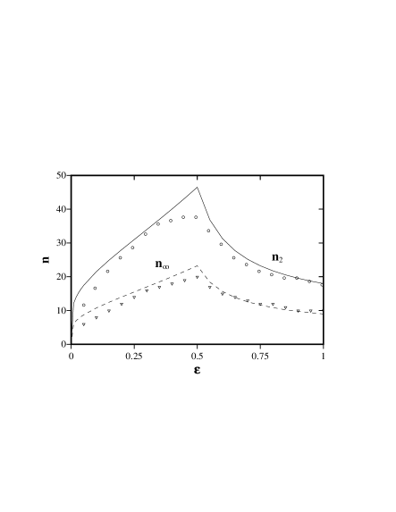
Figure 3: The largest length of the lattice, which can be controlled with two pinning sites: the triangles represent the length obtained using $H_{\infty}$ control, the circles show the data, obtained using $H_{2}$ control in Ref. [8], and the curves show theoretical estimates (32) and (34). The noise strength is $\sigma=10^{-14}$ and $a=4.0$.

If however only partial information about the state of the system is available, additional requirements appear. Any control algorithm utilizing output feedback essentially consists of two major stages: observation and control. During the first stage information about the system is collected and processed to recreate the state of the system. During the second stage, control perturbations are applied to bring the system to the desired state. As a result the control scheme should be able to tolerate uncertainties introduced during both the control and the observation stage.

The estimate (32) reflects the requirements imposed by the control stage. Additional requirements, introduced by the observation stage can be similarly estimated using the observability condition,

$${\rm rank}\left[\matrix{C^{\dagger}\quad A^{\dagger}C^{\dagger}\quad\cdots\quad{A^{\dagger}}^{n-1}C^{\dagger}}\right]=n,$$ (33)

which determines whether the state of the system can be extracted from the observed data (5), and for $C=B^{\dagger}$ coincides with the controllability condition.

Careful consideration shows, that the addition of the observation stage effectively doubles both the length of the control cycle and the length of the lattice. As a result, the maximal length of the system, that can be successfully stabilized using $H_{\infty}$ control is halved:

$$n_{\infty}(\sigma)=n_{2}(\sigma)/2.$$ (34)

The maximal length $n_{\infty}(\sigma)$ can be obtained numerically by choosing the fixed point as the initial condition and monitoring the evolution of the system in the presence of noise under control (9). The results are presented in Fig. 3. One can see that the estimate (34) approximates the actual results rather well.

This work was partially supported by the NSF through grant no. DMR-9013984.

References

• [1] C. Lee, J. Kim, D. Bobcock and R. Goodman, โ€œApplications of neural networks to turbulence control for drag reduction,โ€ Physics of Fluids, V 9, N 6, pp.1740-1747, 1997.
• [2] A. Pentek, J. B. Kadtke and Z. Toroczkai, โ€œStabilizing chaotic vortex trajectories - An example of high-dimensional control,โ€ Phys. Lett. A, V 224, N 1-2, pp.85-92, 1996.
• [3] V. Petrov, M. J. Crowley and K. Showalter, โ€œTracking unstable periodic orbits in the Belousov-Zhabotinsky reaction,โ€ Phys. Rev. Lett., V 72, N 18, pp.2955-2958, 1994.
• [4] C. Lourenco and A. Babloyantz, โ€œControl of spatiotemporal chaos in neuronal networks,โ€ Int. J. Neu. Sys, V 7, N 4, pp.507-517, 1996.
• [5] R. O. Grigoriev and M. C. Cross, โ€œControlling physical systems with symmetries,โ€ submitted to Phys. Rev. E.
• [6] K. Kaneko, โ€œPeriod-doubling of kink-antikink patterns, quaziperiodicity in antiferro-like structures and spatial intermittency in coupled logistic lattice - towards a prelude of a field theory of chaos,โ€ Prog. Theor. Phys., V 72, N 3, pp.480-486, 1984.
• [7] G. Hu and Z. Qu, โ€œControlling spatiotemporal chaos in coupled map lattice systemsโ€, Phys. Rev. Lett., V 72, N 1, pp.68-71, 1994.
• [8] R. O. Grigoriev, M. C. Cross and H. G. Schuster, โ€œPinning control of spatiotemporal chaos,โ€ Phys. Rev. Lett., V 79, N 15, pp.2795-2798, 1997.
• [9] K.Zhou, J. C. Doyle and K. Glover, โ€œRobust and optimal control,โ€ Prentice Hall, 1996, chapter 16.
• [10] G. E. Dullerud and S. G. Lall, โ€œA new approach for analysis and synthesis of time varying systems,โ€ in Proc. 1997 IEEE/CDC.