Multiscaling in Models of Magnetohydrodynamic Turbulence

Abstract

From a direct numerical simulation of the MHD equations we show, for the first time, that velocity and magnetic-field structure functions exhibit multiscaling, extended self similarity (ESS), and generalized extended self similarity (GESS). We also propose a new shell model for homogeneous and isotropic MHD turbulence, which preserves all the invariants of ideal MHD, reduces to a well-known shell model for fluid turbulence for zero magnetic field, has no adjustable parameters apart from Reynolds numbers, and exhibits the same multiscaling, ESS, and GESS as the MHD equations. We also study dissipation-range asymptotics and the inertial- to dissipation-range crossover.

The extension of Kolmogorov’s work (K41) [2] on fluid turbulence to magnetohydrodynamic (MHD) turbulence yields [3] simple scaling for velocity ${\bf{v}}\/$ and magnetic-field ${\bf{b}}\/$ structure functions, for distances $r\/$ in the inertial range between the forcing scale $L\/$ and the dissipation scale $\eta_{d}\/$. Many studies have shown that there are multiscaling corrections to K41 scaling in fluid turbulence [4]. Solar-wind data [5] and recent shell-model studies [6, 7] for MHD turbulence yield similar multiscaling. We elucidate this for homogeneous, isotropic MHD turbulence, in the absence of a mean magnetic field, by presenting the first evidence for such multiscaling in a pseudospectral study of the MHD equations in three dimensions (henceforth $3d$MHD). We also propose a new shell model with no adjustable parameters (apart from Reynolds numbers) which displays this multiscaling and reduces to the Gledzer-Ohkitani-Yamada (GOY) shell model [8, 9] for $3d\/$ fluid turbulence when $\bf b=0$. To extract multiscaling exponents we develop the ideas of extended self similarity (ESS) [12, 13] and generalised extended self similarity (GESS) [13, 14] in both real and wave-vector (henceforth $k$) spaces, that have been used in fluid turbulence [12]-[14].

We use the structure functions ${\cal{S}}_{p}^{a}=\langle|{\boldmath{a}}({\bf{x}}+{\bf{r}})-{\boldmath{a}}({\bf{x}})|^{p}\rangle$, where ${\boldmath{a}}\/$ can be ${\bf{v}}$, ${\bf{b}}$, or one of the Elsässer variables ${\bf{Z}}^{\pm}={\bf{v}}\pm{\bf{b}}\/$, ${\bf{x}}$ and ${\bf{r}}$ are spatial coordinates, and the angular brackets denote an average in the statistical steady state. ${\cal S}_{p}^{a}\sim r^{\zeta_{p}^{a}}\/$ at high fluid and magnetic Reynolds numbers $Re\/$ and $Re_{b}\/$, respectively, and for the inertial range $20\eta_{d}\lesssim r<<L\/$. The extension [3] of K41 to homogeneous, isotropic MHD turbulence with no mean magnetic field yields $\zeta_{p}^{a}=p/3\/$. Shell models [6, 7] and solar-wind data [5] have obtained multiscaling in MHD turbulence, i.e., $\zeta_{p}^{a}=p/3-\delta\zeta_{p}^{a}\/$, with $\delta\zeta_{p}^{a}>0\/$ and $\zeta_{p}^{a}\/$ nonlinear, monotonically increasing functions of $p\/$. Work on fluid turbulence suggests [4] an extension of the apparent inertial range if we use ESS [12] and GESS [14]: Thus with ESS, in which $\zeta_{p}^{a}/\zeta_{3}^{a}\/$ follows from ${\cal{S}}_{p}^{a}\sim[{\cal{S}}_{3}^{a}]^{\zeta_{p}^{a}/\zeta_{3}^{a}}\/$, we should expect by analogy that it extends down to $r\simeq 5\eta_{d}$ (as exploited in some MHD shell models [6, 7]). In GESS, which employs ${\cal{G}}_{p}^{a}(r)\equiv{\cal{S}}_{p}^{a}(r)/[{\cal{S}}_{3}^{a}(r)]^{p/3}$ and postulates a form ${\cal{G}}_{p}^{a}(r)\sim[{\cal{G}}_{q}^{a}(r)]^{\rho^{a}_{pq}}$, with $\rho^{a}_{pq}=[\zeta_{p}^{a}-p\zeta_{3}^{a}/3]/[\zeta_{q}^{a}-q\zeta_{3}^{a}/3]$, it has been suggested [14] for fluid turbulence that the apparent inertial range is extended to the lowest resolvable $r\/$; however, $k$-space GESS [13] shows a crossover from inertial- to dissipation-range asymptotic behaviors. GESS has not been used in MHD turbulence so far.

Our studies yield many interesting results: The multiscaling exponents we obtain from $3d$MHD and our shell model studies agree (Figs. 1a and 1b) and $\zeta_{p}^{b}>\zeta_{p}^{Z^{+}}$ $\stackrel{{\scriptstyle>}}{{\sim}}$ $\zeta_{p}^{Z^{-}}>\zeta_{p}^{v}\/$. $\zeta_{p}^{b}\/$ lie close to the She-Leveque (SL) prediction [15] for fluids ($\zeta_{p}^{SL}=p/9+2[1-(2/3)^{p/3}]\/$), but $\zeta_{p}^{v}\/$ lie below it (Fig. 1c) [16]. These differences between velocity and magnetic-field exponents are also mirrored in differences in the probability distribution functions (Fig. 1d) for $\delta v_{\alpha}({\bf{r}})={v_{\alpha}}({\bf{x}}+{\bf{r}})-{v_{\alpha}}({\bf{x}})$ and $\delta b_{\alpha}({\bf{r}})={b_{\alpha}}({\bf{x}}+{\bf{r}})-{b_{\alpha}}({\bf{x}})$. ESS works both with real- and $k$-space structure functions (Fig. 2). To study the latter we postulate $k$-space ESS (for real-space structure functions we use ${\cal{S}}\/$ and ${\cal{G}}\/$ and for their $k-$space analogs (not Fourier transforms) $S\/$ and $G\/$):

$$S_{p}^{a} \equiv \langle|{\boldmath{a}}({\bf{k}})|^{p}\rangle\approx A^{a}_{Ip}(S_{3})^{\zeta^{{}^{\prime}a}_{p}},\;\;L^{-1}\ll k\lesssim 1.5k_{d},$$ (1)

$$S_{p}^{a} \equiv \langle|{\boldmath{a}}({\bf{k}})|^{p}\rangle\approx A^{a}_{Dp}(S_{3})^{\alpha_{p}^{a}},\;\;1.5k_{d}\lesssim k\ll\Lambda,$$ (2)

where $A^{a}_{Ip}\/$ and $A^{a}_{Dp}\/$ are, respectively, nonuniversal amplitudes for inertial and dissipation ranges and $\Lambda^{-1}\/$ the (molecular) length at which hydrodynamics breaks down (cf. [13] for fluid turbulence). We find that $\alpha^{a}_{p}\neq\zeta^{{}^{\prime}a}_{p}\/$. In our shell model $\zeta^{{}^{\prime}a}_{p}=\zeta_{p}^{a}\/$, but our data for $3d$MHD suggest $\zeta^{{}^{\prime}a}_{p}=2(\zeta^{a}_{p}+3p/2)/11\/$ (i.e., $S_{p}^{a}(k)\sim k^{-(\zeta_{p}^{a}+3p/2)}\/$ in the inertial range [17]); the difference arises because of phase-space factors [13].

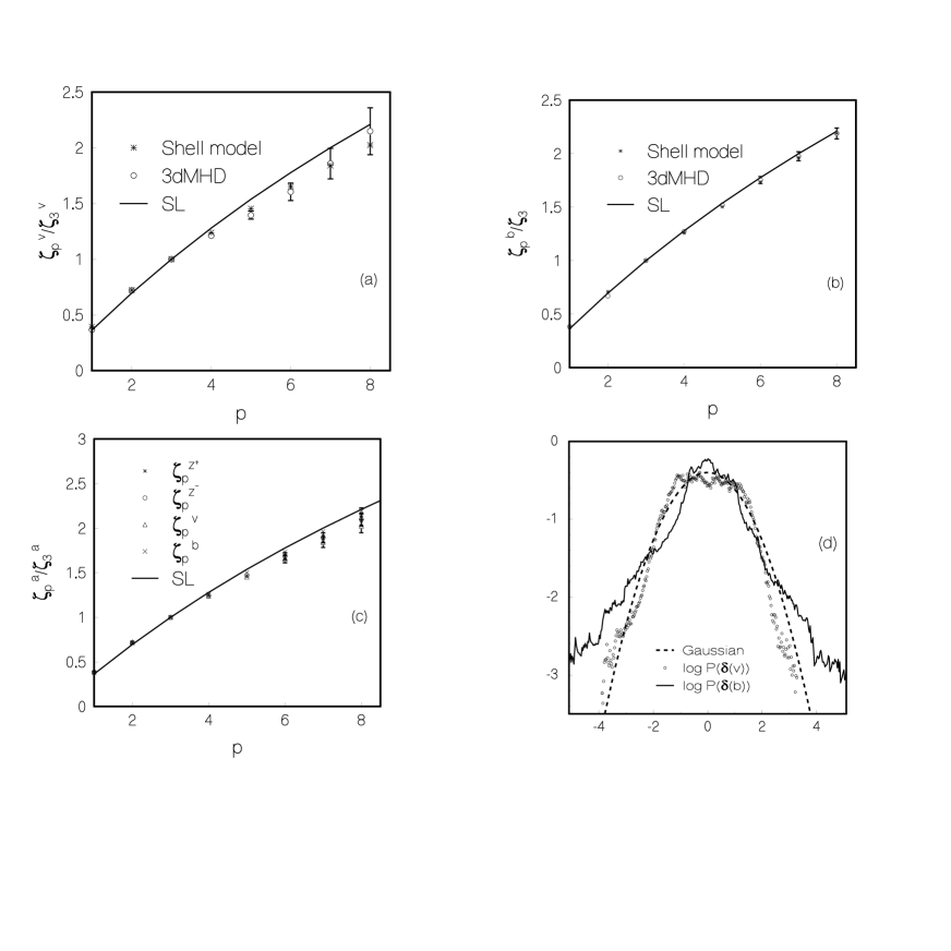
FIG. 1.: (a)-(c)Inertial-range exponents versus $p\/$ from typical $3d$MHD and shell-model runs (Table 1) and their comparison with the SL formula: (a) $\zeta_{p}^{v}/\zeta_{3}^{v}$, (b) $\zeta_{p}^{b}/\zeta_{3}^{b}$, and (c) $\zeta_{p}^{v}$, $\zeta_{p}^{b}$, $\zeta_{p}^{z^{+}}$, and $\zeta_{p}^{z^{-}}$ from SH2. (d) Semilog (base 10) plots of probability distributions $P(\delta v_{\alpha}(r))$ and $P(\delta b_{\alpha}(r))$, with $r$ in the dissipation range; a Gaussian distribution is shown for comparison.

FIG. 2.: Log-log plots (base 10) of $S_{10}^{a}$ versus $S_{3}^{a}$ showing $k$ space ESS for $3d$MHD with (a) $a=v$ and (b) $a=b$. Insets illustrate real-space ESS for $3d$MHD and ESS for our shell model; the lines show the inertial-range asymptotes.

$\zeta^{{}^{\prime}a}_{p}\/$ and $\alpha^{a}_{p}\/$ seem universal (the same for all our runs (Table 1)); $\alpha^{a}_{p}\/$ is close to, but systematically less than, $p/3\/$. The $k\/$ dependences of $S_{p}^{a}$ follow from that of $S^{a}_{3}\/$. We find

$$S^{a}_{3} \approx B^{a}_{I}k^{-\zeta^{a}_{3}-9/2},\;\;L^{-1}\ll k\lesssim 1.5k_{d},$$ (3)

$$S^{a}_{3} \approx B^{a}_{D}k^{\delta^{a}}\exp(-c^{a}k/k_{d}),\;\;1.5k_{d}\lesssim k\ll\Lambda,$$ (4)

where $B^{a}_{I}\/$ and $B^{a}_{D}\/$ are nonuniversal amplitudes (Eq. (2) holds [13] for $3d$MHD; for our shell model the factor $9/2\/$ is absent). Thus all $S^{a}_{p}\sim k^{\theta^{a}_{p}}\exp(-c^{a}\alpha^{a}_{p}k/k_{d})\/$ for $1.5k_{d}\lesssim k\ll\Lambda\/$, with $\theta^{a}_{p}=\alpha^{a}_{p}\delta^{a}\/$ (cf. [13] for fluid turbulence). In Eq.(3) $\delta^{a},c^{a}\/$, and $k_{d}\/$ are not universal. However, we extract the universal part of the inertial- to dissipation-range crossover via our $k\/$-space GESS. We first define $G^{a}_{p}\equiv S^{a}_{p}/(S^{a}_{3})^{p/3}\/$; log-log plots of $G^{a}_{p}\/$ versus $G^{a}_{q}\/$ yield curves with universal, but different, slopes for asymptotes in inertial and dissipation ranges. The inertial-range asymptote has a slope $\rho^{a}_{p,q}\/$ (as in real-space GESS ); the dissipation-range one has a slope $\omega^{a}(p,q)\equiv[\alpha^{a}_{p}-p/3]/[\alpha^{a}_{q}-q/3]\/$. These slopes are universal, but not the points at which the curves move away from the inertial-range asymptote. To obtain a universal crossover scaling function (different for each $(p,q)\/$ pair because of multiscaling) we define $\log(H^{a}_{pq})\equiv D^{a}_{pq}\log(G^{a}_{p})\/$ and $\log(H^{a}_{qp})\equiv D^{a}_{qp}\log(G^{a}_{q})\/$; the scale factors $D^{a}_{pq}=D^{a}_{qp}\/$ are nonuniversal,

FIG. 3.: Log-log plots (base 10) of $H_{9,6}^{v}$ versus $H_{6,9}^{v}$ and (inset) $H_{9,6}^{b}$ versus $H_{6,9}^{b}$, illustrate our GESS showing the universal inertial- to dissipation-range crossover; lines denote inertial-range asymptotes.

but plots of $\log(H^{a}_{pq})\/$ versus $\log(H^{a}_{qp})\/$ collapse onto a universal curve within our error bars for all $k\/$, $Re_{\lambda}\/$, and $Re_{b\lambda}\/$ (Fig. 3).

The MHD equations are [3]

$${\partial{\bf{Z}}^{\pm}\over\partial t}+({\bf Z^{\mp}}.{\bf\nabla)\bf Z^{\pm}}=\nu_{+}\nabla^{2}{\bf Z^{\pm}}+\nu_{-}\nabla^{2}{\bf Z^{\mp}}-{\nabla}p^{*}+{\bf f^{\pm}},$$ (5)

where $\nu_{\pm}\equiv(\nu_{v}\pm\nu_{b})/2\/$, $\nu_{v}\/$ and $\nu_{b}\/$ are, respectively, the fluid and magnetic viscosities, $p^{*}$ is the effective pressure and the density $\rho=1$, ${\bf{f}}^{\pm}\equiv({\bf{f}}\pm{\bf{g}})/2\/$, and ${\bf{f}}\/$ and ${\bf{g}}\/$ are the forcing terms in the equations for $\partial{\bf{v}}/\partial t\/$ and $\partial{\bf{b}}/\partial t\/$. We assume incompressibility and use a pseudospectral method [13] to solve Eq.(5) numerically. We force the first two $k$-shells, use a cubical box with side $L_{B}=2\pi$, periodic boundary conditions, and $64^{3}\/$ modes in runs MHD1 and MHD2 and $80^{3}\/$ modes in run MHD3 (Table 1). We include fluid and magnetic hyperviscosities (i.e., the term $-(\nu_{v}+\nu_{vH}k^{2})k^{2}\/$ in the equation for $\partial{\bf{v}(\bf k)}/\partial t\/$ and the term $-(\nu_{b}+\nu_{bH}k^{2})k^{2}$ in the equation for $\partial{\bf{b}(\bf k)}/\partial t\/$, where $H\/$ stands for hyperviscosity). For time integration we use an Adams-Bashforth scheme (step-size $\delta t$). We use $Re_{\lambda}=v_{rms}\lambda/\nu_{v}$, $Re_{b\lambda}=b_{rms}\lambda/\nu_{b}$, $\lambda_{v}=[\int_{o}^{\infty}E_{v}(k)dk/\int_{o}^{\infty}k^{2}E_{v}(k)dk]^{1/2}$, $\lambda_{b}=[\int_{o}^{\infty}E_{b}(k)dk/\int_{o}^{\infty}k^{2}E_{b}(k)dk]^{1/2}$, $E_{v}(k)\sim S_{2}^{v}(k)k^{2}$ and $E_{b}(k)\sim S_{2}^{b}(k)k^{2}$. Parameters for runs MHD1-3 are given in Table 1, where $\tau_{ea}\equiv L_{B}/a_{rms}\/$ is the box-size eddy-turnover time for field ${\boldmath{a}}\/$ and $\tau_{A}\/$ the averaging time; initial transients are allowed to decay over a period $\tau_{t}\/$. We use quadruple-precision arithmetic; results from our $64^{3}\/$ and $80^{3}\/$ runs are not significantly different.

Shell models for MHD turbulence have been proposed earlier [6, 7, 11], but there is no MHD shell model that enforces all ideal $3d$MHD invariants and which reduces to the GOY shell model for fluid turbulence, when magnetic-field terms are supressed. We present such a model and show that it yields $\zeta_{p}^{a}$ in agreement with those we obtain for $3d$MHD. Our shell-model equations

$${dz_{n}^{\pm}\over\ dt}=ic_{n}^{\pm}-\nu_{+}k_{n}^{2}z_{n}^{\pm}-\nu_{-}k_{n}^{2}z_{n}^{\pm}+f_{n}^{\pm}$$ (6)

use the complex, scalar Elsässer variables $z_{n}^{\pm}\equiv(v_{n}\pm b_{n})\/$, and discrete wavevectors $k_{n}=k_{o}q^{n}$, for shells $n\/$;

$$c_{n}^{\pm} = [a_{1}k_{n}z_{n+1}^{\mp}z_{n+2}^{\pm}+a_{2}k_{n}z_{n+1}^{\pm}z_{n+2}^{\mp}$$ (7)

$$+ a_{3}k_{n-1}z_{n-1}^{\mp}z_{n+1}^{\pm}+a_{4}k_{n-1}z_{n-1}^{\pm}z_{n+1}^{\mp}$$ (8)

$$+ a_{5}k_{n-2}z_{n-1}^{\mp}z_{n-2}^{\pm}+a_{6}k_{n-2}z_{n-1}^{\mp}z_{n-2}^{\pm}]^{*},$$ (9)

which ensures $z_{n}^{+},z_{n}^{-}\sim k^{-1/3}\/$ is a stationary solution in the inviscid, unforced limit [6]-[9] and preserves the $\nu_{+},Z^{+}\leftrightarrow\nu_{-},Z^{-}$ symmetry of $3d$MHD. We fix five of the parameters, $a_{1}-a_{6}\/$, by demanding that our shell-model analogs of the total energy ($\equiv\sum_{n}(|v_{n}|^{2}+|b_{n}|^{2})/2\/$), the cross helicity ($\equiv 1/2\sum_{n}(v_{n}b_{n}^{*}+v_{n}^{*}b_{n})$), and the magnetic helicity ($\equiv\sum_{n}(-1)^{n}|b_{n}|^{2}/k_{n}\/$) be conserved if $\nu_{\pm}=0\/$ and $f_{n}^{\pm}=0\/$; while enforcing the conservation of energy, we also demand [10] that the cancellation of terms occurs as in $3d$MHD. We fix the last parameter by demanding that, if $b_{n}=0\/$ for all $n\/$, our model should reduce to the GOY model, with the standard choice of parameters [9] that conserves fluid helicity in the inviscid, unforced limit. Thus, apart from the Reynolds numbers, our shell model has no adjustable parameters and $a_{1}=7/12,a_{2}=5/12,a_{3}=-1/12,a_{4}=-5/12,a_{5}=-7/12,a_{6}=1/12$, and $q=2\/$. We solve Eq. (6) numerically by an Adams-Bashforth scheme (step size $\delta t$), use 25 shells, force the first $k$-shell [13], set $k_{o}=2^{-4}$, and use $E_{v}=S_{2}^{v}(k_{n})/k_{n}$, $\lambda_{v}=(2\pi/k_{o})[\Sigma_{n}S_{2}^{v}(k_{n})/\Sigma_{n}k_{n}^{2}S_{2}^{v}(k_{n})]^{1/2}$, $\lambda_{b}=(2\pi/k_{o})[\Sigma_{n}S_{2}^{b}(k_{n})/\Sigma_{n}k_{n}^{2}S_{2}^{b}(k_{n})]^{1/2}$, $v_{rms}=[k_{o}\Sigma_{n}S_{2}^{v}(k_{n})/\pi]^{1/2}$ and $b_{rms}=[k_{o}\Sigma_{n}S_{2}^{b}(k_{n})/\pi]^{1/2}$. Parameters for our four runs SH1-SH4 are given in Table 1. These use double-precision arithmetic, but we have checked in representative cases that our results are not affected if we use quadruple-precision arithmetic. As in the GOY model the structure functions $S_{p}(k_{n})$ oscillate weakly with $k_{n}$ because of an underlying three-cycle [9, 10]. These oscillations can be removed either (a) by using ESS plots or (b) by using the structure functions $\Sigma_{n,p}^{a}=\langle{\Im}[a_{n}a_{n+1}a_{n+2}+a_{n-1}a_{n}a_{n+1}/4]^{p/3}\rangle$ [9]. Method (a) yields the exponent ratios $(\zeta_{p}^{a}/\zeta_{3}^{a})$, which we find are universal. Method (b) gives exponents $\zeta^{a}_{p}\/$. These have a mild dependence on $Re_{\lambda}\/$ and $Re_{b\lambda}\/$ but this goes away if we consider the exponent ratios $\zeta^{a}_{p}/\zeta^{a}_{3}\/$, as in the GOY model [13, 18]; thus the asymptotes in our ESS and GESS plots have universal slopes.

The Navier Stokes equation ($3d$NS) follows from $3d$MHD if we set $\bf b=0$ or, equivalently, $Re_{b\lambda}$=0. However, if we start with $Re_{b\lambda}\simeq 0$, the steady state is characterised by the MHD exponents and $Re_{\lambda}/Re_{b\lambda}\simeq O(1)$ (i.e., an equipartition regime)[19]. Since our MHD shell model reduces to the GOY model as $Re_{b\lambda}\rightarrow 0$, we use it to study the fluid turbulence to MHD turbulence crossover, instead of doing costly pseudospectral studies: A small initial value of $Re_{b\lambda}$ yields a transient during which we obtain GOY-model exponents, but eventually the system crosses over to the MHD turbulence steady state [10].

In conclusion, then, we have shown that structure functions in $3d$MHD turbulence display multiscaling, ESS, and GESS, with exponents and probability distributions $P(\delta v_{\alpha}({\bf r}))$ and $P(\delta b_{\alpha}({\bf r}))$ different from those in fluid turbulence. Our new shell model (a) gives the same multiscaling exponents as $3d$MHD and (b) reduces to the GOY shell model as $Re_{b\lambda}\rightarrow 0$. Our ESS and GESS studies help us to uncover an apparently universal crossover from inertial- to dissipation-range asymptotics. It would be very interesting to compare our results with experiments on MHD turbulence, but two points must be borne in mind: (1) solar-wind data might yield multiscaling exponents different from ours because of the presence of a mean magnetic field; (2) the crossover from inertial- to dissipation-range asymptotics might not apply to the solar wind because a hydrodynamic description might break down in the dissipation range [20]. However, our results should apply to MHD systems which show an equipartition regime [3]. It would also be interesting to see whether the agreement of $\zeta_{p}^{b}$ with the SL formula is fortuitous or significant.

We thank J.K. Bhattacharjee and S. Ramaswamy for discussions, CSIR (India) for support, and SERC (IISc, Bangalore) for computational resources.

TABLE I.: The viscosities and hyperviscosities $\nu_{v},\nu_{b},\nu_{vH}\/$ and $\nu_{bH}\/$, the Taylor-microscale Reynolds numbers $Re_{\lambda}\/$ and $Re_{b\lambda}\/$, the box-size eddy-turnover times $\tau_{ev}\/$ and $\tau_{eb}\/$, the averaging time $\tau_{A}\/$, the time over which transients are allowed to decay $\tau_{t}\/$, and $k_{d}\/$ (dissipation-scale wavenumber) for our $3d$MHD runs ($k_{max}=32\/$ for MHD1 and MHD2 and $k_{max}=40\/$ for MHD3) and shell-model runs SH1-4 ($k_{max}=2^{25}k_{0}\/$). The step size($\delta t\/$) is 0.02 for MHD1-3, $2.10^{-5}$ for SH1-2, and $10^{-4}\/$ for SH3-4. Note that $\tau_{ev}\simeq 8\tau_{I}\/$ the integral time for our MHD runs.

Run	$\nu_{v}$	$\nu_{vH}$	$\nu_{b}$	$\nu_{bH}$	$Re_{\lambda}$	$Re_{m\lambda}$	$\tau_{ev}/\delta t\/$	$\tau_{ev}/\delta t\/$	$\tau_{t}/\tau_{ev}\/$	$\tau_{A}/\tau_{ev}\/$	$k_{max}/k_{d}\/$
MHD1	$8\cdot 10^{-4}$	$7\cdot 10^{-6}$	$10^{-3}$	$8\cdot 10^{-6}$	$\simeq 24.8$	$\simeq 14.3$	$\simeq 8.8\cdot 10^{3}\/$	$\simeq 6\cdot 10^{3}\/$	$\simeq 2\/$	$\simeq 2.3\/$	$\simeq 1.83\/$
MHD2	$8\cdot 10^{-4}$	$9\cdot 10^{-6}$	$8\cdot 10^{-4}$	$9\cdot 10^{-6}$	$\simeq 24.1$	$\simeq 18.1$	$\simeq 8.8\cdot 10^{3}\/$	$\simeq 5.6\cdot 10^{3}\/$	$\simeq 2\/$	$\simeq 2.3\/$	$\simeq 1.83\/$
MHD3	$8\cdot 10^{-4}$	$9\cdot 10^{-6}$	$8\cdot 10^{-4}$	$9\cdot 10^{-6}$	$\simeq 26$	$\simeq 19.6$	$\simeq 7.9\cdot 10^{3}\/$	$\simeq 4.8\cdot 10^{3}\/$	$\simeq 1\/$	$\simeq 2.2\/$	$\simeq 2.22\/$
SH1	$10^{-9}$	$0$	$10^{-9}$	$0$	$\simeq 4.6\cdot 10^{8}$	$\simeq 7.8\cdot 10^{8}$	$\simeq 10^{7}\/$	$\simeq 6\cdot 10^{6}\/$	$\simeq 50\/$	$\simeq 450\/$	$\simeq 2^{5}\/$
SH2	$10^{-8}$	$0$	$10^{-8}$	$0$	$\simeq 4.3\cdot 10^{7}$	$\simeq 6.5\cdot 10^{7}$	$\simeq 10^{7}\/$	$\simeq 6\cdot 10^{6}\/$	$\simeq 50\/$	$\simeq 450\/$	$\simeq 2^{8}\/$
SH3	$10^{-6}$	$0$	$2\cdot 10^{-6}$	$0$	$\simeq 4\cdot 10^{6}$	$\simeq 3\cdot 10^{6}$	$\simeq 2\cdot 10^{6}\/$	$\simeq 10^{6}\/$	$\simeq 500\/$	$\simeq 2500\/$	$\simeq 2^{10}\/$
SH4	$4\cdot 10^{-6}$	$0$	$10^{-6}$	$0$	$\simeq 1.2\cdot 10^{5}$	$\simeq 1\cdot 10^{6}$	$\simeq 10^{6}\/$	$\simeq 1.7\cdot 10^{6}\/$	$\simeq 500\/$	$\simeq 3000\/$	$\simeq 2^{11}\/$

REFERENCES

• [1] Also at Jawaharlal Nehru Centre for Advanced Scientific Research, Bangalore, India.
• [2] A. N. Kolmogorov, C. R. Acad. Sci. USSR 30, 301 (1941).
• [3] D. Montgomery in Lecture Notes on Turbulence, eds. J. R. Herring and J. C. McWilliam (World Scientific, Singapore, 1989); D. Biskamp in Nonlinear Magnetohydrodynamics, eds. W. Grossman, D. Papadopoulos, R. Sagdeev, and K. Schindler (Cambridge University Press, Cambridge, 1993).
• [4] For recent reviews see: K. R. Sreenivasan and R. A. Antonia, Ann. Rev. Fluid Mech., 29, 435 (1997); and S. K. Dhar, A. Sain, A. Pande, and R. Pandit, Pramana - J. Phys., 48, 325 (1997).
• [5] R. Grauer, J. Krug, and C. Marliani, Phys. Lett., 195, 335 (1994).
• [6] D. Biskamp, Phys. Rev. E, 50, 2702 (1994) also finds $\zeta_{p}^{b}>\zeta_{p}^{v}$, for $p=2\/$, in a shell model.
• [7] V. Carbone, Phys. Rev. E, 50, R671 (1994).
• [8] E.B. Gledzer, Sov. Phys. Dokl., 18, 216, (1973): K. Ohkitani, and M. Yamada, Prog. Theor. Phys., 81, 329 (1989).
• [9] L. Kadanoff, D. Lohse, and J. Wang, Phys. Fluids, 7, 517 (1995).
• [10] A. Basu and R. Pandit, unpublished.
• [11] C. Gloaguen, J. Leorat, A. Pouquet, and R. Grappin, Physica, 17D, 154 (1985).
• [12] R. Benzi, S. Ciliberto, R. Trippiccione, C. Baudet, F Massaioli, and S. Succi, Phys. Rev. E, 48, R29 (1993).
• [13] S. K. Dhar, A. Sain, and R. Pandit, Phys. Rev. Lett., 78, 2964 (1997).
• [14] R. Benzi, L. Biferale, S. Ciliberto, M. Struglia, and R. Trippiccione, Europhys. Lett., 32, 709 (1995).
• [15] Z. S. She and E. Leveque, Phys. Rev. Lett., 72, 336 (1994).
• [16] We use the SL formula as a convenient parametrization for the multiscaling exponents in fluid turbulence.
• [17] For a heuristic justification for fluid turbulence see [13].
• [18] E. Leveque and Z. S. She, Phys. Rev. Lett., 75, 2690 (1995).
• [19] Thus in a renormalization-group calculation $Re_{b\lambda}$ should appear as a relevant operator that takes the system from the $3d$NS-turbulence fixed point to the $3d$MHD-turbulence fixed point.
• [20] E. Marsch in Reviews in Modern Astronomy, 4, ed. G. Klare (Springer Verlag, Berlin, 1991).