[

Chaos of the Relativistic Parametrically Forced van der Pol Oscillator

Abstract

A manifestly relativistically covariant form of the van der Pol oscillator in $1+1$ dimensions is studied. We show that the driven relativistic equations, for which $x$ and $t$ are coupled, relax very quickly to a pair of identical decoupled equations, due to a rapid vanishing of the “angular momentum” (the boost in $1+1$ dimensions). A similar effect occurs in the damped driven covariant Duffing oscillator previously treated. This effect is an example of entrainment, or synchronization (phase locking), of coupled chaotic systems. The Lyapunov exponents are calculated using the very efficient method of Habib and Ryne. We show a Poincaré map that demonstrates this effect and maintains remarkable stability in spite of the inevitable accumulation of computer error in the chaotic region. For our choice of parameters, the positive Lyapunov exponent is about 0.242 almost independently of the integration method.

]

The chaotic behavior of a covariant relativistic generalization of the classical Duffing oscillator in $1+1$ dimensions has been studied recently [4, 5]. This system is completely integrable, since both the total “mass” (the value of the invariant generator of dynamical evolution) and the hyperbolic “angular momentum” (the generator of Lorentz transformations in $1+1$ dimensions) are conserved. Under non-stationary perturbation, including a friction term as well, however, the stable and unstable orbits in the phase space separate and cross (infinitely many times).

Some general features of the resulting chaotic orbits were discussed in ref.[4], such as the phenomena of period doubling and the apparent existence of a strange attractor [6]. In ref.[5], analytic solutions were studied for the unperturbed problem in the neighborhood of the separatrix, and it was shown that the perturbative Melnikov criterion[7] for homoclinic chaos was satisfied. It was found that along with chaotic behavior in space, there is chaos in time in such a system, with perhaps profound implications for our perception of the nature of dynamical processes.

In this paper, we study a manifestly covariant dynamical system with no Hamiltonian structure, i.e., a covariant form of the van der Pol oscillator. The model was originally introduced by van der Pol[8] to describe the triode electronic oscillator, and used by van der Pol and van der Mark as a model for heart rhythms[9]. The van der Pol equation was introduced before chaos was systematically defined or studied, and it became one of the first examples to be analyzed for chaotic behavior and associated entrainment phenomena [10, 11, 12, 13]. This system carries intrinsic (coordinate dependent) friction; if this term vanishes, one obtains the structure of an ordinary harmonic oscillator. The method of Melnikov is not applicable for the van der Pol system, since there is no homoclinic orbit associated with the unperturbed problem. We shall therefore calculate the Lyapunov exponents to demonstrate the chaotic behavior [7].

It was observed in the case of the relativistic Duffing problem that the $x$ and $t$ modes, viewed as two coupled systems, could converge, in the presence of friction, to a single Duffing type oscillator (the “angular momentum” converges to zero). This convergence is an example of the entrainment (sometimes called “phase locking”) of two coupled chaotic systems. We observe a similar behavior in the relativistic van der Pol equations. It is conceivable that nonconservative relativistic electronic systems have similar properties, providing examples of fundamental interest for the entrainment, or synchronization (phase locking) properties of such chaotic systems [14].

As for the Duffing oscillator, we add a driving force that conserves the “angular momentum”, so that there is minimal distortion introduced by such a term. We find, as for the Duffing oscillator, that the time and space modes coalesce, with resulting loss of independent degrees of freedom. The resulting one-dimensional system does not coincide precisely with the usual nonrelativistic case; the forcing term appears proportional to the dependent variable ($x(\tau)$ or $t(\tau)$). This term must be then shifted to the non-linear coefficient of the dependent variable in the van der Pol equation (previous studies have considered driving terms in the coefficient of the $\dot{x}$[15]). It was therefore necessary to investigate the chaotic structure of the resulting system independently of previous studies.

Although the chaotic behavior of the usual van der Pol system is difficult to observe, we found that in our case, the usual methods utilizing, for example, Poincaré maps, clearly demonstrate the more complex chaotic character of this system. Moreover, we employ a method given by Habib and Ryne [16] for the study of the Lyapunov exponents to confirm the chaotic nature of the system; this method is very effective in studying a system of this type, i.e., a system for which the local linearization can be described in terms of a Hamiltonian form.

The rapid relaxation of the dissipative relativistic system to a system closely related to the nonrelativistic form is of interest in itself in providing an example of how dissipation can induce an effectively nonrelativistic dynamics (through entrainment of the time and space modes). A similar phenomena occurs, as mentioned above, in the dissipative form of the Duffing oscillator under certain conditions [4].

Following the classical relativistic mechanics of Stueckelberg [17], and its extension [18] to the many body problem, one can define a relativistic invariant evolution function $K$ (analogous to the nonrelativistic Hamiltonian), which generates “Hamilton-like” equations:

$$\frac{dx_{i}^{\mu}}{d\tau}=\frac{\partial K}{\partial p_{i\mu}},\qquad\frac{dp_{i}^{\mu}}{d\tau}=-\frac{\partial K}{\partial x_{i\mu}},$$ (1)

where $p_{i}^{\mu}$ and $x_{i}^{\mu}$ are the energy-momentum and spacetime coordinates ($i=1\dots N$, $\mu=0,1$, with metric -, +) and $\tau$ is a universal invariant parameter for motion in $2N$-dimensional phase space.

Consider the two body problem with a potential that depends on the invariant distance between them, for which the corresponding evolution function, $K$, may be written as:

$$K=\frac{p_{1}^{\mu}p_{1\mu}}{2M_{1}}+\frac{p_{2}^{\mu}p_{2\mu}}{2M_{2}}+V(\rho^{2}),$$ (2)

where $\rho^{2}$ is the Poincaré invariant

$$\rho^{2} = (x_{1}^{\mu}-x_{2}^{\mu})(x_{1\mu}-x_{2\mu})$$ (3)

$$= (x_{1}-x_{2})^{2}-(t_{1}-t_{2})^{2}.$$ (4)

It is possible to write the two body problem as a function of center of mass and the relative motion between the bodies (in a way similar to nonrelativistic mechanics):

$$K=K_{c.m.}+K_{rel}$$ (5)

$$K_{c.m.}=\frac{P^{\mu}P_{\mu}}{2M}$$ (6)

$$K_{rel}=\frac{p^{\mu}p_{\mu}}{2m}+V(\rho^{2}),$$ (7)

where

$$M=M_{1}+M_{2}\qquad m=\frac{M_{1}M_{2}}{M_{1}+M_{2}}$$ (8)

$$P^{\mu}=p_{1}^{\mu}+p_{2}^{\mu}\qquad p^{\mu}=\frac{M_{2}p_{1}^{\mu}-M_{1}p_{2}^{\mu}}{M_{1}+M_{2}}$$ (9)

$$X^{\mu}=\frac{M_{1}x_{1}^{\mu}+M_{2}x_{2}^{\mu}}{M_{1}+M_{2}}\qquad x^{\mu}=x_{1}^{\mu}-x_{2}^{\mu}.$$ (10)

FIG. 1.: The angular momentum, $M^{01}(\tau)$, of the typical cases where there is a) exponential growth followed by an oscillatory exponential decay of $M^{01}(\tau)$ where $\dot{M}_{0}^{01}M_{0}^{01}>0$, b) oscillatory exponential decay of $M^{01}(\tau)$ where $\dot{M}_{0}^{01}M_{0}^{01}\leq 0$

The equations of motion in the new variables are

$$\frac{dx^{\mu}}{d\tau}=\frac{\partial K_{rel}}{\partial p_{\mu}}\qquad\frac{dp^{\mu}}{d\tau}=-\frac{\partial K_{rel}}{\partial x_{\mu}}$$ (11)

$$\frac{dX^{\mu}}{d\tau}=\frac{\partial K_{c.m.}}{\partial P_{\mu}}\qquad\frac{dP^{\mu}}{d\tau}=0;$$ (12)

the system separates to two equations describing the center of mass and the relative motion of the system.

FIG. 2.: The $(y,z)$ plane of fig. 1a and b. The inset in fig. 2b shows an enlargement of the turning point from the initial point to the final linear curve.

The equation for the nonrelativistic externally forced van der Pol oscillator is [8, 9] :

$$\ddot{x}+\alpha(x^{2}-1)\dot{x}+kx=g\cos\omega t,$$ (13)

where the right hand side corresponds to an external driving force. Although there is no Hamiltonian which generates this equation, we may nevertheless consider its relativistic generalization in terms of a relative motion problem, for which there is no evolution function $K$.

In this paper, we study the relativistic generalization of Eq. (13) in the form

$$\ddot{x}^{\mu}+\alpha(\rho^{2}-1)\dot{x}^{\mu}+x^{\mu}=0,$$ (14)

or, in terms of components,

$$\ddot{x}+\alpha(x^{2}-t^{2}-1)\dot{x}+kx= 0$$ (15)

$$\ddot{t}+\alpha(x^{2}-t^{2}-1)\dot{t}+kt= 0,$$ (16)

where $x,t$ are the relative coordinates of the two body system. The term $\dot{x}$ can be understood as representative of friction due to radiation, as for damping due to dipole radiation of two charged particles, proportional to the relative velocity $\dot{x}^{\mu}$ in the system [5]. To study the existence of chaotic behavior on this system, we add a driving force to the system (it already contains dissipation intrinsically) in such a way that it does not provide a mechanism in addition to the dissipative terms for the change of “angular momentum” (this quantity is conserved by eq. (14) with $\alpha=0$)

$$M^{01}=x^{0}p^{1}-x^{1}p^{0}=m(t\dot{x}-x\dot{t}).$$ (17)

To achieve this, we take a driving force proportional to $x^{\mu}$, so that (15) becomes

$$\ddot{x}+\alpha(x^{2}-t^{2}-1)\dot{x}+kx = fx\cos\omega\tau$$ (18)

$$\ddot{t}+\alpha(x^{2}-t^{2}-1)\dot{t}+kt = ft\cos\omega\tau.$$ (19)

The derivative of the angular momentum can be evaluated in terms of these equations as

$$\frac{dM^{01}}{d\tau}=-\alpha(x^{2}-t^{2}-1)M^{01}.$$ (20)

In contrast to exponential decay of the angular momentum that was shown in Duffing oscillator [4], one cannot see clearly whether eq. (20) reflects such decay or not. Exponential decay of $M^{01}$ means that after a relatively short time $M^{01}$ goes to zero, and that $x$ becomes proportional to $t$ ($x=\beta t$). Thus, in this case, the two coupled equations would actually reduce to one equation. In order to simplify the investigation of eqs. (18) and (19), one can introduce two symmetric equations by subtracting and adding them, to obtain

$$\ddot{y}+\alpha(yz-1)\dot{y}+ky = fy\cos\omega\tau,$$ (21)

$$\ddot{z}+\alpha(yz-1)\dot{z}+kz = fz\cos\omega\tau,$$ (22)

where $y=x-t$ and $z=x+t$. Eqs. (21), (22) are completely symmetric and it is clear that if one starts from initial conditions $(y_{0},\dot{y}_{0})=\beta(z_{0},\dot{z}_{0})$ the equations behave identically (up to a multiplicative constant). In this case, the angular momentum, $M^{01}=\frac{m}{2}(z\dot{y}-y\dot{z})$, is zero, and hence $y=\beta z$. The derivative of $M^{01}$ in the new variables is,

$$\frac{dM^{01}}{d\tau}=-\alpha(yz-1)M^{01}.$$ (23)

For the system (21), (22), $M^{01}$ appears to converge, in actual computations, to zero independently of initial conditions. In fact, there are three typical behaviors of $M^{01}$ before it reaches zero: (a) An exponential growth (or oscillatory exponential growth) of $|M^{01}|$ followed by exponential decay (or oscillatory exponential decay) to zero, a scenario which occurs when $\dot{M}_{0}^{01}M_{0}^{01}>0$. (b) An exponential decay (or oscillatory exponential decay) of $|M^{01}|$ to zero, which occurs when $M^{01}\neq 0$ and $\dot{M}_{0}^{01}M_{0}^{01}\leq 0$. (c) $M^{01}$ is zero initially and remains zero.

In fig. 1 we present the behaviors of cases (a) and (b). The numerical calculation of eqs. (21), (22), were performed using the adaptive time step fifth-order Cash-Karp Runge-Kutta method [19], and by fixed time step forth-order Runge-Kutta method [19]. We choose $m=1$ for the mass and $\omega=2.466$, $\alpha=1$, $k=1$ and $f=10$. The initial conditions used in fig. 1a were $y_{0}=1$, and $\dot{y}_{0}=z_{0}=\dot{z}_{0}=-1$ ($M_{0}^{01}=1$ and $\dot{M}_{0}^{01}=2$), and it is easy to observe the initial exponential growth and the succeeding oscillatory exponential decay to zero. In fig. 1b a typical behavior of case (b) is shown. The initial conditions are $y_{0}=3$, $\dot{y}_{0}=2$, $z_{0}=\frac{1}{2}$ and $\dot{z}_{0}=0$ ($M_{0}^{01}=\frac{1}{2}$ and $\dot{M}_{0}^{01}=\frac{1}{4}$), and the typical behavior of an exponential oscillatory decay to zero is shown. If fig. 2a and 2b we show the $(y,z)$ plane of fig. 1a and 1b which the solutions converge to a linear curve after a short time and then continue with oscillations on this line. Hence we also see in the phenomenon of entrainment in the van der Pol case.

After the angular momentum reaches zero there is no reason to investigate the two coupled eqs. (21), (22), which actually become uncoupled since the variables are proportional. Thus, one is left with the equation (we henceforth replace $\tau$ by the familiar designation $t$ appropriate to the nonrelativistic case):

$$\ddot{x}+\alpha(x^{2}-1)\dot{x}+kx=fx\cos(\omega t).$$ (24)

A class of equations including eq. (24) were studied by Schmidt and Tondl [20] for the case for which both damping and nonlinear terms, as well as the homogeneous driving term are taken as small (as can be seen by scaling the dependent variable); they used perturbative techniques to study the instability. Cicogna & Fronzoni [21] have studied the modification of chaos of the Duffing oscillator using an additional forcing term which can be proportional to $x$; a similar structure occurs in ref. [4], as mentioned above. Such a forcing term occurs in the Mathieu equation (as a time-dependent frequency) [22]. Our study is not restricted to small coefficients; it utilizes numerical methods of wider applicability.

In the following we will show the chaotic properties of eq. (24), including the complex shape of the trajectory itself (which is reflected by a continuous frequency spectrum), and the fractal form of the Poincaré map, which in our case is just $(x(t_{n}),\dot{x}(t_{n}))$ where $t_{n}=t_{0}+nT$ ($T=\frac{2\pi}{\omega}$ and $n$ is an integer number larger then $0$). The chaotic behavior is verified by the existence of a positive Lyapunov exponent.

There exist several methods for calculating Lyapunov exponents from a set of first order differential equations [23, 24]. However, we preferred a new method developed by Habib and Ryne [16], which is based on a technique using symplectic matrices. The symplectic computation of Lyapunov exponents is applicable whenever the linearized dynamics is Hamiltonian (which true for our system). The basic advantage of the symplectic method is that it avoids the renormalization and reorthogonalization procedures necessary in the usual techniques, and thus, leads to fast and accurate results (the method avoids an additional error which can be caused by the renormalization and reorthogonalization procedures).

According to the method of Habib and Ryne one linearizes the system, as a first step in the computation of Lyapunov exponents. In our case, the linearization of eq. (24) is

$$\ddot{\delta}+\alpha(x_{0}^{2}-1)\dot{\delta}+(2\alpha x_{0}\dot{x}_{0}+k-f\cos\omega t)\delta=0,$$ (25)

where $\delta=x-x_{0}$ and $x_{0}$ is the fiducial trajectory [24]. Following Habib and Ryne, we change the variable to $\Delta=\delta\exp(-g(t))$, where $\dot{g}(t)=-\frac{\alpha}{2}(x_{0}^{2}-1)$, so that eq. (25) becomes,

$$\ddot{\Delta}-(\ddot{g}(t)+\dot{g}(t)^{2}-k+f\cos\omega t)\Delta=0.$$ (26)

In order to find the Lyapunov exponents it is necessary to solve two first order differential equations, [16]

$$\frac{d\mu}{dt} = {1\over 2}(s_{22}-s_{11})\cos a$$ (27)

$$\frac{da}{dt} = s_{11}+s_{22}-(s_{22}-s_{11})\sin a\coth\mu.$$ (28)

The Lyapunov exponents are then $\pm\mu/t$, where $t$ is sufficiently large. These equations are obtained as follows. In the general case of a Hamiltonian of quadratic form,

$$H({\bf Z},t)={1\over 2}\sum_{i,j=1}^{2m}s_{ij}Z_{i}Z_{j},$$ (29)

where ${\bf Z}=(q_{1},q_{2},\dots,q_{m},p_{1},p_{2},\dots,p_{m})$, the canonically conjugate coordinates and momenta, the equation of motion for ${\bf Z}(t)=M(t){\bf Z}(0)$ implies that

$$\frac{d}{dt}M\tilde{M}=JSM\tilde{M}-M\tilde{M}SJ,$$ (30)

where

$$J=\pmatrix{0&{\bf 1}\cr-{\bf 1}&0\cr}$$ (31)

and $S=(s_{ij})$. The equations (28) are then obtained for a system with one degree of freedom (in the case that there is no term of the type $qp$ in the Hamiltonian), by recognizing that the most general form of the symplectic matrix $M$ is given by

$$M=e^{\mu(B_{2}\cos a+B_{3}\sin a)}e^{bB_{1}},$$ (32)

where $B_{1}=i\sigma_{1}$, $B_{2}=\sigma_{2}$ and $B_{3}=\sigma_{3}$, and $\{\sigma_{i}\}$ are the Pauli matrices.

In the case of eq. (33), the $s_{ij}$ are :

$$s_{11} = -(\ddot{g}(t)+\dot{g}(t)^{2}-k+f\cos\omega t)$$ (33)

$$= \alpha x_{0}\dot{x}_{0}-\frac{\alpha^{2}}{4}(x_{0}^{2}-1)^{2}+k-f\cos\omega t,$$ (34)

$$s_{22} = 1.$$ (35)

After finding the Lyapunov exponents, $\lambda_{\pm}=\pm\lim_{t\to\infty}{\mu(t)/t}$, of eq. (26) using eqs. (28), one must find the Lyapunov exponents of the original system, eq. (25). By recognizing that asymptotically eq. (26) is $\Delta_{\pm}=\delta_{\pm}\exp(-g(t))=\exp{\lambda_{\pm}t}$, one can then find the Lyapunov exponents of eq. (25) [16]:

$$\chi_{\pm}=\lim_{t\to\infty}{1\over t}(g(t)\pm\mu(t)).$$ (36)

It is possible to summarize the Lyapunov exponents calculation of our system (eq. (24)) by five first ordered differential equations:

$$\frac{dx_{0}}{dt} = p_{0},$$ (37)

$$\frac{dp_{0}}{dt} = -\alpha(x_{0}^{2}-1)p_{0}-kx_{0}+fx_{0}\cos{\omega t},$$ (38)

$$\frac{dg}{dt} = -\frac{\alpha}{2}(x_{0}^{2}-1),$$ (39)

$$\frac{d\mu}{dt} = {1\over 2}(1-\alpha x_{0}p_{0}+\frac{\alpha^{2}}{4}(x_{0}^{2}-1)^{2}-k+f\cos{\omega t})\cos{a},$$ (40)

$$\frac{da}{dt} = 1+\alpha x_{0}p_{0}-\frac{\alpha^{2}}{4}(x_{0}^{2}-1)^{2}+k-f\cos{\omega t}-$$ (42)

$$(1-\alpha x_{0}p_{0}+\frac{\alpha^{2}}{4}(x_{0}^{2}-1)^{2}-k+f\cos{\omega t})\sin{a}\coth{\mu},$$

and the Lyapunov exponents can be found by eq. (36). The first two equations calculate the fiducial trajectory. The third relation is needed for the calculation of the Lyapunov exponents. The last two equations are just the explicit form of eqs. (28).

In order to locate some parameter values which lead to chaotic behavior, one must map the positive Lyapunov exponent in parameter space. Since our parameter space is represented in four dimensions , the mapping of chaotic regions are quite difficult and it is necessary to focus on one or two parameters; we choose $\alpha$ to be the varying parameter since it controls the nonlinearity of the system.

FIG. 3.: Lyapunov exponents as a function of $\alpha$ for a) positive Lyapunov exponent, b) negative Lyapunov exponent.

In fig. 3 we show Lyapunov exponents as a function of $\alpha$ (the other parameter values are $\omega=2.466$, $k=1$, $f=5$). We draw the Lyapunov exponents after $200000$ time units. The larger Lyapunov exponent is shown in fig. 3a, and it is easy to see that it becomes positive in a small region of the range of $\alpha$. One can also identify some periodicity in $\chi_{+}(\alpha)$ multiplied by a decaying envelope. This “periodicity” gives a clue about some intrinsic frequency which resonates with the “external” frequency, $\omega$. However, it seems that the gap between the chaotic regions is not exactly constant. A negative Lyapunov exponent is shown in fig. 3b. As expected, the absolute value of the negative Lyapunov exponent is much larger than the positive one. The negative Lyapunov exponent decreases approximately linearly with $\alpha$ (not including some regions parallel to chaotic regions with positive Lyapunov exponent) since $\alpha$ controls the dissipation of the system.

One of the fundamental questions in the numerical solution of chaotic systems is the validity of the numerical results. Since in every numerical integration there is an accumulative error, the integrated trajectory separates from the real trajectory in a very short distance. According to chaos theory, a nearby trajectory can generate a completely different trajectory (nearby trajectories actually separate exponentially), thus, one cannot guarantee the accuracy of the numerical calculation. The numerical trajectory is method dependent, and more than this, is accuracy dependent (if one changes the integration accuracy the trajectory behaves differently). One should expect, moreover, sensitivity to the integration method (or, equivalently, sensitivity to accuracy of the integration) if the system is chaotic, a fact which can used as an additional sign of chaotic behavior. Thus, it is clear that one cannot rely on the numerical results. The question is whether one can rely on the global characteristic values, such as, Lyapunov exponents. It seems that the answer is that one can indeed trust the global values, although the local behavior is not assured . It seems that although the trajectories behave differently they appear to “move” on the attractor; they have the same global characteristic exponents. The influence of this sensitivity can be seen in fig. 3a. One recognizes easily that there is a clear smooth behavior of $\chi_{+}(\alpha)$ when it is less then zero (the system is not chaotic and nearby trajectories do not separate exponentially); once the exponent becomes positive $\chi_{+}(\alpha)$ becomes less smooth.

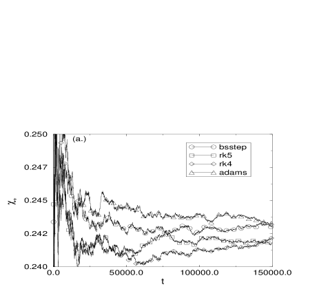
FIG. 4.: Convergence of Lyapunov exponents to a constant value, as a function of $t$, using four different integration methods for a) positive Lyapunov exponent, b) negative Lyapunov exponent.

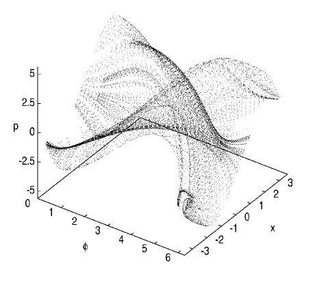
FIG. 5.: The attractor of relaxed relativistic van der Pol oscillator.

In order to verify the claim that the Lyapunov exponents are the same for different integration techniques, we compare the results between four different methods: 1. Bulirsch-Stoer method using Richardson extrapolation [19] (denoted by bsstep); 2. adaptive stepsize fifth Runge-Kutta method using Cash-Karp parameters [19] (denoted by rk5); 3. fourth Runge-Kutta method [19] (denoted by rk4); and 4. Adams integration method [26]. We choose $\alpha=1.149$ since it gives the largest positive Lyapunov exponent as seen in fig. 3a. The Lyapunov exponents are shown in fig. 4 and it is clear that all methods lead to approximately the same exponents; $\chi_{+}=\approx 0.242$, $\chi_{-}=\approx-4.286$.

One can find other signs of chaotic behavior with the parameters used in fig. 3 ($\omega=2.466$, $k=1$ and $f=5$), and taking $\alpha=1.149$. In fig. 5 the real phase space, $(\phi,x,p)$, where $\phi=\omega t$ mod $2\pi$, is shown. It can be seen clearly that the trajectory is very complicated and does not return to itself. The phase space lies on a surface with some width; a fact which suggests a noninteger fractal dimension. Using the Kaplan and Yorke conjecture [27], the fractal dimension would be :

$$D_{L}=j+{\sum_{i=1}^{j}\lambda_{i}\over|\lambda_{j+1}|}\approx 2+{0.242\over 4.286}\approx 2.06$$ (43)

where $j$ is defined by the condition that $\sum_{i=1}^{j}\lambda_{i}>0$ and $\sum_{i=1}^{j+1}\lambda_{i}<0$ (the Lyapunov exponent in the time direction is, of course, zero).

FIG. 6.: The complex behavior of $x(t)$ (we have used the notation $t$ instead of $\tau$ to describe the decoupled system).

No clear periodicity is seen in $x(t)$ , as shown in fig. 6. The Fourier transform of $x(t)$ (fig. 7) shows a continuous frequency spectrum, which is a sign of chaotic behavior. In addition, there is an approximate linear decay of the logarithm of the power spectrum, a fact which is connected to the exponential decay of the autocorrelation function [28] (we also checked the autocorrelation itself and its envelope indeed decays exponentially). One sees a peak in the neighborhood of $1$, which is the frequency of the undamped and unforced oscillator. One would expect resonant behavior in the neighborhood of half the driving frequency ($\Omega={\omega\over 2}$) on the basis of a comparison with the Mathieu equation [22]. In our case, there is a apparent resonant region around this frequency $\Omega\sim 1.233$.

Despite the difficulties mentioned above, we succeeded to draw a Poincaré map for eq. (24). The map in this case is just the points on the plane $\phi=0$, and can be written as $(x(t_{n}),p(t_{n}))$, where $t_{n}={2\pi\over\omega}n$ and $n$ is a nonnegative integer. The map is drawn using two different methods : rk4, and the Adams method; one obtains the same mapping structure. This is a surprising result since, as mentioned before, one can not be sure of the accuracy of the trajectory $x(t)$ due to accumulation error which leads to a different trajectory behavior. The map shown in fig. 8 shows smooth curves with stretching and folding phenomenon (more fine structure is seen in the inset). The map is antisymmetric, and obviously has a fractal dimension $\approx 1.06$ (following eq. (43) and ignoring the time direction).

FIG. 7.: The power spectrum of fig. 6. The dashed line indicates the free oscillator frequency, i.e., $\Omega=\sqrt{k}=1$.

The entrainment phenomenon observed between space and time chaotic modes, both for the Duffing [4] and van der Pol case, for which $x$ and $t$ appear to approach exponentially to a smooth linear relation, even though both $x$ and $t$ remain chaotic, presents a mechanism for the rapid convergence of damped relativistic systems to their classical limit. Underlying this smooth behavior of $x(t)$, one might expect to see a characteristic property of the radiation field reflecting the chaotic behavior of both $x$ and $t$, in such systems.

We further remark that the stability of the Poincaré plots of fig. 8 indicates that computational deviations of $x$ are compensated to reach a smooth curve by deviations in $t$. This stability is analogous to the stability of the calculation of the Lyapunov coefficients along a fiducial curve that is calculated with an inevitable error. Both the Poincaré plots and Lyapunov calculations appear to reflect properties of the attractor rather that the local computed orbit.

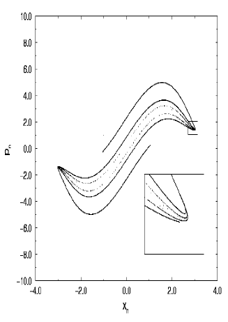
FIG. 8.: The Poincaré map of the relaxed relativistic van der Pol equation. The inset shows an enlargement of the map.

We would like to thank W.C. Schieve for suggesting this problem and discussions in the initial stages of this work.

REFERENCES

- [1]
- [2] email-address: ashkenaz@mail.biu.ac.il
- [3] email-address: larry@larry.tau.ac.il
- [4] W.C. Schieve and L.P. Horwitz, Phys. Lett. A 156, 140 (1991).
- [5] L.P. Horwitz and W.C. Schieve, Phys. Rev. A 46, 743 (1992).
- [6] J. Guckenheimer and P. Holmes, Nonlinear Oscillations, Dynamical Systems, and Bifurcations of Vector Fields, (Springer Verlag, New York, 1986).
- [7] V.K. Melnikov, Trans. Mosc. Math. Soc. 12, 1 (1963).
- [8] B. Van der Pol, Phil. Mag. (7) 2, 978 (1926).
- [9] B. Van der Pol and Van der Mark, Phil. Mag. (7) 6, 763 (1928).
- [10] M.L. Cartwright and J.E. Littlewood, J. London Math. Soc. 20, 180 (1945).
- [11] E.A. Jackson, Perspectives of Nonlinear Dynamics vol. 1, (Cambridge University, Cambridge 1991).
- [12] N. Kryloff and N. Bogliuboff, Introduction to Non-Linear Mechanics, Annals of Math. Studies, (Princton Univ. Press, 1947); N. Bogoliuboff and Y.A. Mitropolsky, Asymptotic Method in the Theory of Nonlinear Oscillations, (Gordon and Breach, 1961).
- [13] L.M. Sander, Scientific American 256, 94 (1987).
- [14] R.C. Hilborn, Chaos and Nonlinear Dynamics, (Oxford Univ. Press, New York, 1994).
- [15] R.Shaw, Z. Naturf. 36a, 80 (1981).
- [16] S. Habib and R. Ryne, Phys. Rev. Lett. 74, 70 (1995).
- [17] E.C.G. Stueckelberg, Helv. Phys. Acta. 14, 322, 588 (1941).
- [18] L.P. Horwitz and C. Piron, Helv. Phys. Acta. 48, 316 (1973).
- [19] W.H. Press, S.A. Teukolsky, W.T. Vetterling, and B.P. Flannery, Numerical Recipes in C, 2nd ed. (Cambridge University, Cambridge, 1995).
- [20] G. Schmidt and A. Tondl, Non-linear Vibrations, (Cambridge University Press, London, 1986).
- [21] G. Cicogna and L. Fronzoni, Phys. Rev. E 47, 4585 (1993).
- [22] P. Glendinning, Stability, instability and chaos: an introduction to the theory of nonlinear differential equations, (Cambridge University, Cambridge, 1994).
- [23] For a comparison of different methods for computing Lyapunov exponents see: K. Geist, U. Parlitz and W. Lauterborn, Prog. Theor. Phys. 83, 875 (1990).
- [24] For a basic computer algorithm for Lyapunov exponents calculations from a set of first order differential equations, as well as a calculation of Lyapunov exponents from a single time series, see : A. Wolf, J.B. Swift, H.L. Swinney and J.A. Vastano, Physica D 16, 285 (1985).
- [25] J.M. Greene, J. Math. Phys. 20, 1183 (1979).
- [26] NAG (Fortran Library).
- [27] J.L. Kaplan and J.A. Yorke, in: Functional Differential Equations and Approximations of Fixed Points, Lecture Notes in Mathematics 730, eds. H.-O. Peitgen and H.-O. Walther (Springer Verlag, Berlin, 1979).
- [28] M. Tabor, Chaos and Integrability in Nonlinear Dynamics, (John Wiley & Sons, N.Y., 1989).