Quantal-Classical Duality and the Semiclassical Trace Formula

Abstract

We consider Hamiltonian systems which can be described both classically and quantum mechanically. Trace formulas establish links between the energy spectra of the quantum description, and the spectrum of actions of periodic orbits in the Newtonian description. This is the duality which we investigate in the present paper. The duality holds for chaotic as well as for integrable systems.

Billiard systems are a very convenient paradigms and we use them for most of our discussions. However, we also show how to transcribe the results to general Hamiltonian systems. In billiards, it is natural to think of the quantal spectrum (eigenvalues of the Helmholtz equation) and the classical spectrum (lengths of periodic orbits) as two manifestations of the properties of the billiard boundary. The trace formula express this link since it can be thought of as a Fourier transform relation between the classical and the quantum spectral densities. It follows that the two point statistics of the quantal spectrum is related to the two point statistics of the classical spectrum via a double Fourier transform. The universal correlations of the quantal spectrum are well known, consequently one can deduce the classical universal correlations. In particular, an explicit expression for the scale of the classical correlations is derived and interpreted. This allows a further extension of the formalism to the case of complex billiard systems, and in particular to the most interesting case of diffusive system. The effects of symmetry and symmetry-breaking are also discussed.

The concept of classical correlations allows a better understanding of the so-called diagonal approximation and its breakdown. It also paves the way towards a semiclassical theory that is capable of global description of spectral statistics beyond the breaktime. An illustrative application is the derivation of the disorder-limited breaktime in case of a disordered chain, thus obtaining a semiclassical theory for localization. We also discuss other applications such as the two-cell systems, periodic chains and localization theory in more than one dimension.

A numerical study of classical correlations in the case of the 3D Sinai billiard is presented. Here it is possible to test some assumptions and conjectures that underly our formulation. In particular we gain a direct understanding of specific statistical properties of the classical spectrum, as well as their semiclassical manifestation in the quantal spectrum.

We also analyze the spectral duality for integrable systems, and show that the Poissonian statistics of both the classical and the quantum spectra can be traced to the same origin.

I Introduction

Trace formulas manifest an intimate link between two seemingly unrelated spectra which pertain to the quantum and the classical descriptions of a given Hamiltonian system. The quantum spectrum of eigenenergies is described in terms of the spectral density

$$d_{qm}(E;\hbar)\ =\ \sum_{n=1}^{\infty}\delta\left[E-E_{n}(\hbar)\right]$$ (1.1)

and it depends parametrically on Planck’s constant. The classical spectrum of actions characterizes the set of periodic manifolds at an energy $E$. These are isolated periodic orbits (POs) in case of a chaotic system or periodic (rational) tori in case of integrable system. The actions are expressed as contour integrals in the $2d$ dimensional phase space

$$S_{\alpha}(E)\ =\ \oint_{C_{\alpha}}\sum_{i=1}^{d}p_{i}{\rm d}q_{i}$$ (1.2)

where $C_{\alpha}$ is a closed trajectory on the periodic manifold (PO in the case of a chaotic system). Note that the periodic manifolds, as well as their actions, depend parametrically on the chosen energy $E$. One can define a density of classical actions

$$d_{cl}(S;E)\ =\ \sum_{\alpha}A_{\alpha}\delta\left[S-S_{\alpha}(E)\right]$$ (1.3)

and with an appropriate choice of the coefficients $A_{\alpha}$ the trace formulas are expressed as

$$d_{qm,osc}(E;\hbar)\ \sim\ (2\pi\hbar)^{-f}\sum_{\alpha}A_{\alpha}{\rm e}^{iS_{\alpha}/\hbar}\ =\ (2\pi\hbar)^{-f}\int{\rm e}^{iS/{\hbar}}d_{cl,osc}(S;E)\ {\rm d}S$$ (1.4)

where $d_{qm,osc}\equiv d_{qm}-\bar{d}_{qm}$ and $\bar{d}_{qm}(E;\hbar)$ is is the smoothed spectral density. The power $f$ depends on the dimensionality of the classical periodic manifold: it is $1$ for isolated POs in chaotic systems, and $(d+1)/2$ for periodic tori in integrable systems. The symbol $\sim$ indicates that the right hand side provides the leading term in an asymptotic expansion in $\hbar$ of the left hand side. This is the semiclassical trace formula (SCTF) which is the main object of our discussion. Explicit expressions for the semiclassical $A_{\alpha}$ coefficients for chaotic and for integrable systems were derived by Gutzwiller [6] and Berry and Tabor [8], respectively. It should be noted, that there are few cases where the symbol $\sim$ can be replaced by an equality sign. One example is the Selberg trace formula for the modular domains in the hyperbolic plane. A second example is the rectangular billiards in any dimension. The higher terms in the $\hbar$ expansion are known in some cases [11] and are introduced by adding to $A_{\alpha}$ a power series in $\hbar$. For a general billiard there is a theorem by Andersson and Melrose [5] that states that exist $A_{\alpha}$ for which (1.4) is an exact equality.

It should be emphasized that both sides of the SCTF (1.4) are distributions rather than functions. Therefore one cannot use it directly but only after it is integrated over an appropriate test or window function. Once this is done one can use the SCTF to study the quantal spectral statistics of a finite spectral interval in terms of the properties of the classical dynamics which are embedded in $d_{cl}$ [17, 18, 27]. Consider the two point spectral form factor, which is calculated for the spectral window $w(E-\bar{E})$ whose effective width is $\Delta E$. For $t>0$

$$K(t;\bar{E})\ \equiv\ \frac{1}{\bar{d}_{qm}\Delta E}\left|\sum_{n}w(E-E_{n}){\rm e}^{iE_{n}t/\hbar}\right|^{2}$$ (1.5)

The inner summation over $n$ can be replaced by an integration over $E$ with the density $d_{qm}(E)$. Substituting the SCTF for $d_{qm}(E)$ and assuming that $\Delta E$ is sufficiently small on the classical scale, but large enough on the quantal scale, one obtains:

$$K(t;\bar{E})\ \approx\ \frac{(2\pi\hbar)^{-f}}{\bar{d}_{qm}\Delta E}\left|\sum_{\alpha}\tilde{w}(t-T_{\alpha})A_{\alpha}{\rm e}^{iS_{\alpha}(\bar{E})/\hbar}\right|^{2}$$ (1.6)

Here $\tilde{w}$ is the Fourier transform of the energy window function, and it picks out of the PO sum only those POs whose period $T_{\alpha}$ approach $t$ to within $\hbar/\Delta E$. Note that the sum over POs in (1.6) absolutely converges for a suitably chosen window. The absolute square of the sum in (1.6) is composed of two kinds of contributions. The contribution of the diagonal terms is

$$K_{D}(t,\bar{E})=\frac{(2\pi\hbar)^{-f}}{\bar{d}_{qm}\Delta E}\sum_{\alpha}\left[\tilde{w}(t-T_{\alpha})\right]^{2}\left|A_{\alpha}\right|^{2}$$ (1.7)

and the contribution of the non diagonal terms is

$$K_{ND}(t;\bar{E})=\frac{(2\pi\hbar)^{-f}}{\bar{d}_{qm}\Delta E}\sum_{\alpha\neq\beta}\tilde{w}(t-T_{\alpha})\tilde{w}(t-T_{\beta})\ A_{\alpha}A_{\beta}^{\star}\ {\rm e}^{i[S_{\alpha}-S_{\beta}]/\hbar}$$ (1.8)

Berry [17] was the first to observe that for times much shorter than the Heisenberg time $t_{H}(\bar{E})=2\pi\hbar\bar{d}_{qm}$ the diagonal contribution dominates. Using the Hannay and Ozorio de Almeida sum-rule [12] he was able to reproduce the expression of $K(t)$ for $t<t_{H}$ as derived from random matrix theory (RMT) for generic chaotic systems, and the expression derived for a Poissonian spectrum for generic integrable systems. This approach has been generalized later [18] by observing that the diagonal sum is related to the classical probability to return [18].

The contribution of the non diagonal sum (1.8) is by no means small for $t\geq t_{H}$. As a matter of fact it should contain a term which (for chaotic systems) cancels the monotonically increasing $K_{D}\propto t$ so that the correct asymptotic behavior $K(t)\rightarrow 1$ is achieved for $t>t_{H}$. This asymptotic behavior reflects the fact that the density $d_{qm}(E)$ corresponds to a discrete spectrum. Note that if $d_{qm}(E)$ were smooth, then $K(t)$ would asymptotically vanish. The asymptotic non-zero value is therefore a hallmark of the discreteness. Argaman et al. [19] have related $K_{ND}(t)$ to the two point correlations of the classical spectrum. The distribution of the classical actions differences $[S_{\alpha}-S_{\beta}]$, with the restriction that the periods are confined to the vicinity of the time $t$, has been determined by taking an inverse Fourier transform of (1.8) in the variable $1/\hbar$. For chaotic systems in 2D, the classical two-point correlations scales into a universal function, provided the action differences are expressed in units of ${1\over t}\left.{\partial\Omega\over\partial E}\right|_{\bar{E}}$, where $\Omega(E)$ is the volume of the phase space with energy $\leq E$. This prediction was checked numerically for a few chaotic systems, and its relation to the Hardy-Littlewood conjecture on pair correlations of primes was also discussed [4].

The important new element in [19] was that a hitherto unnoticed correlations between classical actions were derived from the SCTF, and from the phenomenological observation that the spectral statistics of quantum chaotic systems reproduce the results of RMT. (See also the discussion by Dahlqvist [43]). It should be emphasized that it is crucial to assume that the SCTF indeed reproduces discrete energy levels (‘convergence’ in the sense of distributions), else the argument for the existence of ‘classical correlations’ loses its validity. Thus, there is an inherent connection between the quest for classical correlations, and the wonder concerning to the mathematical soundness (‘convergence’) of the SCTF. This point has been raised by Gutzwiller [7] who introduced the term ‘third entropy’ in order to refer to the statistical properties of the actions.

The conjecture of classical action-correlations leads naturally to the introduction of some fundamental questions:

• What is the dynamical origin of the correlations between classical actions? In other words, how can one derive these correlations from purely classical considerations, without recourse to the SCTF and quantum mechanics ?

• The classical density consists of $\delta$ functions which are supported by the actions of the periodic manifolds, and weighted by complex coefficients whose magnitude as well as phase differ from orbit to orbit. How much of the expected correlations reflect the distribution of actions, and what is the rôle (if any) of the correlations amongst the coefficients themselves or amongst the actions and the coefficients?

• Periodic orbits proliferate exponentially with their periods. Excluding non generic degeneracies, this implies an exponentially large density of actions of POs. Previous numerical checks [13] have convincingly shown that on the scale of the (exponentially small) nearest actions separation, the action spectrum is Poissonian. How is this compatible with action correlations?

• What is the classical phase-space significance of the classical correlation scale (geometrical interpretation in case of billiards)? What is the way to generalize the scaling relation for action correlations beyond 2D ? What are the modifications that are required in case of complex (e.g. diffusive) systems ?

Even though the non diagonal contribution to the form factor attracted much attention in the past few years, all the studies so far avoided the direct confrontation with action correlations and the questions listed above. Khmelnitskii and coworkers [24] as well as Altshuler et al [23] computed the form factor for disordered (chaotic) systems by employing techniques other than the semiclassical theory. Bogomolny and Keating [25] effectively replaced the contributions of POs with $t>t_{H}/2$ by composite POs constructed in a special (synthetic) way. Miller [22] has deduced action correlations of composite POs from unitarity, and derived from them the classical correlations of primitive POs.

The purpose of the present paper is to pick up again the subject of action correlations from the point where it was left by [19]. We shall introduce an explicit formulation of the quantal-classical duality concept, and will extend it to the general case of either integrable or chaotic systems with $d$ degrees of freedom. We shall refer to generic as well as to non-generic circumstances. At a later stage we shall discuss the modifications that are required in the application to complex (e.g. diffusive) systems. The formulation of quantal-classical duality and the associated heuristic understanding of classical correlations thus paves the way towards a global semiclassical theory of spectral statistics that goes beyond the diagonal approximation. We use from now on the term ‘classical correlations’ or ‘classical PO-correlations’ rather than the term ‘action correlations’. Sometimes, the latter term is misleading. Some of the results were already reported by D. Cohen [21]. They are discussed and further developed in the present paper.

Some remarks on the method of presentation are in order. Most of the discussion will be carried out for billiard systems. Billiards are particularly convenient since they are scaling systems. Because of this property, the SCTF can be simplified by considering the quantum wavenumbers instead of the energies, and in the classical description the length of the PO replaces the action and the time, (since one can always choose $m=v=1$). Once the theory for billiards is presented, we shall show how to transcribe it for any Hamiltonian system.

In section II the general formulation of the quantal-classical duality is presented. The SCTF is used in order to derive the relation between the two point statistics of the quantal and the classical spectra. In particular, the universal classical correlation scale $\lambda$ is identified. This section contains a detailed discussion of the statistical procedure and its relation to the energy-time plane. We discuss the crossover from the ‘classical regime’ to the ‘quantal regime’ and the proper definition of the breaktime follows naturally. The applicability of the semiclassical theory beyond the (irrelevant) Ehrenfest ‘log’-time is clarified. The role of non-universal features is discussed as well.

In section III we give an interpretation of the classical correlation scale, and introduce a statistical model for rigidity in terms of ‘families’. Then we use various arguments and the notions of ‘classification’ and ‘similarity’ in order to reveal the actual structure of the classical spectrum. Finally we make some observations concerning the origin of classical correlations.

Some of our observations concerning classical correlations are further supported by the numerical study of section VI. There we have carried out a detailed analysis of the quantum and classical spectra of the Sinai billiard in 3D, for which we possess substantial and immaculate data bases [39]. This analysis provides for the first time a clue to the basic problem – the derivation of the classical PO-correlations based on a purely classical argument rather than on the semiclassical duality.

Section IV extends the formulation of section II to the general case of either chaotic or integrable Hamiltonian systems. For generic integrable system we discuss the dual Poissonian nature of both the quantal and the classical spectra. (See also [8, 9, 10]). The general strategy is further illustrated by referring to specific examples, namely, the Riemann zeros and the 3D torus. The cubic 3D torus is particularly interesting due to its non-genericity and is analyzed in detailed.

Besides the mathematically oriented questions that concern the existence of classical correlations, there is also the practical hope to extend the semiclassical theory beyond the diagonal approximation. Classical PO-correlations become most significant in the analysis of complex systems since they lead to relatively short breaktime scales that are not related to the universal Heisenberg time. In section V we make use of the physical insight gained in the discussion of classical PO-correlations in order to formulate the modifications that are required in order to go beyond the diagonal approximation. A specific example is the quasi-1D classically-diffusive chain. The quantal form factor should correspond either to Anderson-localized eigenstates or to band structure, depending on whether the chain is disordered or periodic. These genuine quantal effects are due to interference, hence the non-diagonal terms play a crucial role. One may question the feasibility of having PO-theory for the spectral properties in such circumstances. Thus, our interest in complex systems is twofold. On the one hand we develop a semiclassical theory which is not limited by the diagonal approximation. On the other hand we test the limits of the semiclassical approach. We use our present level of understanding of the SCTF and of classical PO-correlations in order to demonstrate that the SCTF should be effective also in the study of complex systems. The emergence of a non-universal volume-independent breaktime in case of a disordered systems is an obvious consequence of the formulation.

II General Theory

The semiclassical trace formula (SCTF) relates the quantal spectrum of energy levels to the classical spectrum of periodic orbits (POs). As explained in the introduction the SCTF can be utilized in order to derive a semiclassical expression for the quantal form factor. The purpose of this section, following [21], is to introduce an explicit formulation of the quantal-classical duality concept. The reader should notice that a clear and explicit formulation of the quantal-classical duality requires modifications of some common notations. In particular, we find it convenient neither to unfold the quantal spectrum nor to scale the quantal form factor. It is also most convenient to adhere to the standard Fourier transform conventions. The new formulation, which will be discussed thoroughly in the following section, promotes the understanding of the classical correlation scale, illuminates the crossover from the ‘classical’ to the ‘quantal’ regime, and sheds new light on the significance of the statistical procedure.

A The Semiclassical Trace Formula

The quantal spectrum $\{k_{n}\}$ consists of real positive eigen-wavenumbers that are defined by the Helmholtz equation $(\nabla^{2}+k^{2})\psi=0$ with the appropriate boundary conditions. The average (smoothed) density is found via Weyl [3] law whose leading order term is

$$K_{Q}(k)\ \equiv\ \left\langle\sum_{n}2\pi\delta(k{-}k_{n})\right\rangle_{\delta k}\ \approx\ C_{d}\Omega\ k^{d{-}1}\ \ \ \ \ \ \ \ ,\left[C_{d}=\left(2^{d{-}2}\pi^{\frac{d}{2}{-}1}\Gamma(\frac{d}{2})\right)^{-1}\right]\ \ \ .$$ (2.1)

In the above $\Omega$ is the volume of the billiard, and $d$ is the dimensionality. The statistical averaging $\langle...\rangle$ implies smoothing using a window of width $\delta k$. Further discussion of the statistical procedure will appear at later subsections. It is natural to define a density $\rho_{qm}(k)$ that corresponds to the quantal spectrum, namely

$$\rho_{qm}(k)\ \equiv\ 2\pi[d_{qm}(k)-\bar{d}_{qm}(k)]\ \equiv\ \left.\sum_{n}2\pi\delta(k{-}k_{n})\right|_{osc}\ \ \ \ \ .$$ (2.2)

The subscript $osc$ implies that the smooth component of the density is being subtracted. This is done in order to simplify the subsequent formulation. Furthermore, in order to facilitate the application of Fourier transform (FT) conventions we define $\rho(-k)=\rho(k)$ for $k<0$. The factor $2\pi$ has been incorporated in the above definition for the same reason.

The classical spectrum $\{L_{j}\}$ of periodic orbits (POs) is defined as the set of all the primitive lengths $L_{p}$ and their repetitions $0{<}r$ such that $L_{j}=rL_{p}$. For a simple chaotic billiard, due to ergodicity, the so called ‘Hannay and Ozorio de Almeida sum rule’ implies

$$K_{D}(L)\ \equiv\ \left\langle\sum_{j}|A_{j}|^{2}\delta(L-L_{j})\right\rangle_{\delta L}\ \approx\ L\ \ \ \ ,$$ (2.3)

where a smoothing window of width $\delta L$ is being used. The generalization of this sum rule to complex systems is discussed later in section V-B. The weighting factors are $|A_{j}|^{2}=L_{p}^{2}/|\det(M_{p}^{r}{-}I)|$ where $M$ is the monodromy matrix. These weighting factors decay exponentially with $L$, namely $|A_{j}|^{2}\sim L^{2}\exp(-\sigma L)$, where $\sigma$ is the average Lyapunov exponent. Hence (using (2.3)) one deduces that the actual smoothed density $\bar{d}_{cl}(L)$ of POs grows exponentially as $\exp(\sigma L)/L$. It is natural to define a weighted density $\rho_{cl}(L)$ that corresponds to the classical spectrum, namely

$$\rho_{cl}(L)\ \equiv\ [d_{cl}(L)-\bar{d}_{cl}(L)]\ \equiv\ \left.\sum_{j}A_{j}\delta(L{-}L_{j})\right|_{osc}\ \ \ \ ,\ \ \ \ \ \ \ \ \ \left[\ A_{j}=\frac{L_{p}}{\sqrt{|\det(M_{p}^{r}{-}I)|}}\ \mbox{e}^{+i\frac{\pi}{2}\nu_{j}}\ \right]\ \ \ \ \ .$$ (2.4)

The instability amplitudes $A_{j}$ are endowed with a phase factor that contains the effective Maslov index $\nu_{j}=r\nu_{p}$ which includes repetitions and the boundary contribution due to reflections. As in the analogous definition of the quantal density, we adhere to standard FT conventions: The classical density satisfies the symmetry relation $\rho(-L)=\rho^{*}(L)$, and the sign in front of the Maslov index is positive. A negative sign would be incorporated if time domain FT conventions ($-i\omega t$) rather than space domain FT conventions ($+ikx$) were used. The former are used in the general derivation of Gutzwiller [6].

The semiclassical trace formula (SCTF) relates the quantal density $\rho_{qm}(k)$ to the classical density $\rho_{cl}(L)$. The relation is simply

$$\rho_{qm}(k)\ \ =\ \ {\cal FT}\ \rho_{cl}(L)$$ (2.5)

Disregarding the smooth part, the SCTF (2.5) states that $\sum_{n}2\pi\delta(k{-}k_{n})=\sum_{j}A_{j}\exp(-ikL_{j})$. Its Fourier transformed version is $\sum_{n}\exp(ik_{n}L)=\sum_{j}A_{j}\delta(L{-}L_{j})$. However, if the two sides of the trace formula were multiplied by a window function then the Fourier transformed version would be (See remark [1]),

$$\sum_{n}w(k_{n}{-}k)\exp(ik_{n}L)\ =\ \mbox{e}^{ikL}\sum_{j}\tilde{w}(L_{j}{-}L)A_{j}\exp(-ikL_{j})\ \ \ ,$$ (2.6)

where $\tilde{w}$ is the Fourier transformed window. This version of the trace formula is manifestly symmetric and is also more convenient for numerical studies. From a mathematical point of view the latter version of the SCTF is superior due to its convergence property.

B Duality of Two Points Statistics

In order to study the statistical properties of either the quantal or the classical spectrum it is natural to define the corresponding two point correlation functions. It follows from the SCTF that the two-point statistics of the quantal spectrum is related to the two-point statistics of the classical spectrum via a double Fourier transform, namely $\langle\rho_{qm}(k)\rho_{qm}(k^{\prime})\rangle\ =\ {\cal F\!T}{\cal F\!T}\ \langle\rho_{cl}(L)\rho_{cl}(L^{\prime})\rangle$. Without the averaging operation $\langle...\rangle$, the latter relation is mathematically trivial and useless. In the sequel, we shall argue that the equality holds non-trivially as a statistical relation, meaning that the averages on both sides of the equality can be carried out independently. We postpone for a moment both the discussion of this point, and the precise definition of the averaging procedure. We turn first to introduce some formal definitions.

The two point correlation function of the quantal spectrum is defined as follows

$$R_{qm}(k,\epsilon)\ \equiv \ \left\langle\rho_{qm}\left(k{-}\frac{\epsilon}{2}\right)\ \rho_{qm}\left(k{+}\frac{\epsilon}{2}\right)\right\rangle$$ (2.7)

$$= \left\langle\ \sum_{nm}\ \delta\left(\epsilon{-}(k_{m}{-}k_{n})\right)\ \ \delta\left(k{-}\frac{k_{n}{+}k_{m}}{2}\right)\ \right\rangle\ -\ (2\pi\bar{d}_{qm}(k))^{2}$$ (2.8)

$$= 2\pi K_{Q}(k)\cdot[\delta(\epsilon)-b(\epsilon;k)]\ \ \ .$$ (2.9)

It is a function of $\epsilon$ and it depends parametrically on $k$. Sometimes it is convenient to notationally suppress the parametric dependence. We shall frequently use the brief notation $R_{qm}(\epsilon)$. The smoothed density squared has been subtracted, and therefore $R_{qm}(\epsilon)$ approaches zero asymptotically for $\epsilon\rightarrow\infty$. The $\delta(\epsilon)$ term is due to the self correlations ($n=m$) of the levels. The function $b(\epsilon)$ can be interpreted as the ‘probability’ density for finding a vacancy at a range $\epsilon$ from some reference level. It should have normalization equal to one since the quantal spectrum is characterized by a finite rigidity scale, still it may possess negative parts if there is a clustering effect. The spectral form factor $K_{qm}(k,L)$ is the FT of $R_{qm}(k,\epsilon)$ in the variable $\epsilon{\leadsto}L$.

The two point correlation function of the classical spectrum is defined analogously as follows

$$R_{cl}(x,L)\ \equiv \ \left\langle\rho_{cl}\left(L{-}\frac{x}{2}\right)\ \rho_{cl}\left(L{+}\frac{x}{2}\right)\right\rangle$$ (2.10)

$$= \ \left\langle\ \sum_{ij}A_{i}^{*}A_{j}\ \delta(x{-}(L_{j}{-}L_{i}))\ \ \delta\left(L{-}\frac{L_{i}{+}L_{j}}{2}\right)\ \right\rangle\ -\ (\bar{d}_{cl}(L))^{2}$$ (2.11)

$$= \ K_{D}(L)\cdot[\delta(x)-p(x;L)]\ \ .$$ (2.12)

It is a function of $x$ and it depends parametrically on $L$. Sometimes it is convenient to notationally suppress the parametric dependence on $L$. The smoothed density squared has subtracted, and therefore $R_{cl}(x)$ approaches zero asymptotically for $x\rightarrow\infty$. The $\delta(x)$ term is due to the self correlations of POs. The function $p(x)$ can be interpreted as the ‘probability’ density for finding a vacancy at a range $x$ from some reference PO. It should have normalization equal to one if the the spectrum is characterized by a finite rigidity scale. We shall argue later that this is indeed the case. Still, it may possess negative parts if there is a clustering effect.

With the above definitions the relation between the the quantal two points statistics and the classical two points statistics can be written in the following form

$$R_{qm}(k,\epsilon)\ =\ {\cal F\!T}{\cal F\!T}\ R_{cl}(x,L)\ \ \ ,$$ (2.13)

where the first ${\cal F\!T}$ corresponds to $x\leadsto k$ and the second ${\cal F\!T}$ corresponds to $L\leadsto\epsilon$. Alternatively

$$K_{qm}(k,L)\ =\ K_{cl}(k,L)\ \ \ .$$ (2.14)

Thus, on semiclassical grounds, if the function $K(k,L)$ is viewed as a function of $L$ then it equals the quantal form factor, while if it is viewed as a function of $k$ it equals the classical form factor. It also follows that if the quantal spectrum is characterized by non-trivial correlations, then also the classical spectrum should be characterized by some non-trivial correlations.

We turn now to define the meaning of the statistical averaging. It is most convenient to do it in the $(k,L)$ plane. Namely,

$$\langle f(k,L)\rangle_{\delta k\delta L}\ \equiv\ \frac{1}{\delta k\delta L}\int_{k{-}\frac{\delta k}{2}}^{k{+}\frac{\delta k}{2}}\int_{L{-}\frac{\delta L}{2}}^{L{+}\frac{\delta L}{2}}f(k^{\prime},L^{\prime})\ dk^{\prime}dL^{\prime}\ \ \ \ \ \ .$$ (2.15)

In the $(k,\epsilon)$ plane the $\delta L$ averaging implies multiplying $R_{qm}(\epsilon)$ with a cutoff function whose width is $2\pi/\delta L$. Analogously, in the $(x,L)$ plane the $\delta k$ averaging implies multiplying $R_{cl}(x)$ with a cutoff function whose width is $2\pi/\delta k$. The semiclassical relation holds trivially provided the same window parameters are used in both sides of the equation, namely

$$K_{qm}(k,L,\delta k,\delta L)\ =\ K_{cl}(k,L,\delta k,\delta L)\ \ \ \ .$$ (2.16)

If the further condition $2\pi\ll\delta k\delta L$ is satisfied, then this relation can be cast into the form

$${\frac{2\pi}{\delta k}}\left\langle\left|\matrix{\ \scriptscriptstyle\cr\displaystyle\sum\exp(ik_{n}L)\cr\scriptscriptstyle k{-}\frac{\delta k}{2}<k_{n}<k{+}\frac{\delta k}{2}\ \ \ }\right|^{2}\right\rangle_{\scriptscriptstyle\delta L}\!\!={\frac{1}{\delta L}}\left\langle\left|\matrix{\ \scriptscriptstyle\cr\displaystyle\sum A_{j}\exp(ikL_{j})\cr\scriptscriptstyle L{-}\frac{\delta L}{2}<L_{j}<L{+}\frac{\delta L}{2}\ \ \ \ }\right|^{2}\right\rangle_{\scriptscriptstyle\delta k}\ \ \ \ .$$ (2.17)

The condition $2\pi\ll\delta k\delta L$ guarantees that the two points statistics is not sensitive to the exact value of the window parameters. It follows that we may choose the window parameters that appear in both sides of (2.16) independently. In this sense (2.14) becomes a statistically meaningful relation. Further discussion of the $(k,L,\delta k,\delta L)$ space will appear at later subsections.

The summations in the above statistical relation are the same which occur in the calculation of the SCTF. The number of terms in these summations is finite as in (2.6), due to the windows which are used. Equation (2.17) is in some sense the ‘squared’ version of (2.6), the main difference being that in the latter case $\delta L=0$ on the left hand side, while $\delta k=0$ on the right hand side. Furthermore, in (2.6) the $L$-window should be related to the $k$-window by a Fourier transform. Later we shall discuss one more aspect of the relation of (2.17) to the SCTF.

C Universal correlations

The quantal spectrum is characterized by a universal correlation scale $\Delta(k)$. For a simple ballistic billiard it simply coincides with the average level spacing. Random Matrix Theory (RMT) further determines the appropriate universal scaling function, namely

$$b(\epsilon;k)\ \ =\ \ \frac{1}{\Delta(k)}\ \hat{b}\left(\frac{\epsilon}{\Delta(k)}\right)\ \ \ \ .$$ (2.18)

From this scaling relation one derives the corresponding scaling relation of the quantal form factor, namely

$$K_{qm}(k,L)\ =\ L_{H}(k)\cdot\hat{K}_{0}(L/L_{H}(k))\ \ ,$$ (2.19)

where $L_{H}(k)=2\pi/\Delta(k)=K_{Q}(k)$ is the Heisenberg time. For the Gaussian Unitary Ensemble (GUE) there is a particularly simple result $\hat{K}_{0}(\tau)=\min(\tau,1)$. If there is a time reversal symmetry one should use the result of the Gaussian Orthogonal Ensemble (GOE).

Using analogous strategy, let us assume that the classical spectrum is characterized by some universal correlation scale $\lambda(L)$ such that

$$p(x;L)\ =\ \frac{1}{\lambda(L)}\hat{p}\left(\frac{x}{\lambda(L)}\right)\ \ \ \ ,$$ (2.20)

where $\hat{p}(s)$ is some scaling function. The justification for assuming the above scaling behavior will be discussed in subsection F. For simplicity of presentation it has been assumed that the classical spectrum has no degeneracies. We note however that if time reversal symmetry is taken into account, where for the generic non self tracing orbits the degeneracy is $g=2$, then the scaling relation should be modified by writing $p(x)=-(g{-}1)\delta(x)+(g/\lambda)\hat{p}(x/\lambda)$ so that $R_{cl}(x)=g[\delta(x)-(1/\lambda)\hat{p}(x/\lambda)]$. One may say that this degeneracy constitutes a trivial type of classical correlations.

Taking the Fourier transform of $R_{qm}(\epsilon)$ we have deduced that $K_{qm}(L)$ should have a crossover at the Heisenberg time $L=2\pi/\Delta(k)$. Similarly, taking the Fourier transform of $R_{cl}(x)$ it is obvious that $K_{cl}(k)$ should have a crossover at $k=2\pi/\lambda(L)$. Alternatively, one may say that the crossover should occur when $\lambda(L)$ equals the De-Broglie wavelength $2\pi/k$. However, due to the semiclassical relation (2.14) the latter condition should coincide with the former condition for having a crossover at the Heisenberg time. It follows that $K(k,L)$ has two regimes in the $(k,L)$ plane which are separated by a crossover line whose equation is

$$L=\frac{2\pi}{\Delta(k)}\ \ \ \ \ \ \Leftrightarrow\ \ \ \ \ \ k=\frac{2\pi}{\lambda(L)}\ \ \ \ .$$ (2.21)

Assuming that $\Delta(k)$ and $\lambda(L)$ are monotonic decreasing functions, it follows that the $(k,L)$ plane is divided into a classical low-$L$–large-$k$ regime (C), and a quantal large-$L$–low-$k$ regime (Q). These are illustrated in the left drawing of Fig.1. Using Weyl law $2\pi/\Delta(k)=C_{d}\Omega k^{d{-}1}$, it follows from (2.21) that for a simple ballistic billiard the classical correlation scale should be

$$\lambda_{0}(L,\Omega)\ =\ {2\pi}\left(C_{d}\frac{\Omega}{L}\right)^{1/(d{-}1)}$$ (2.22)

Note that this prediction is independent of any detailed RMT result. For a 2D system, it coincides with the scaling relation of [19] that we have mentioned in the introduction. The validity of (2.22) follows from the validity of the SCTF. The subscript $0$ indicates that the universal (rather than some non-universal) correlation scale were considered here.

FIG. 1.: Regions in the $(k,L,\delta k,\delta L)$ space. The classical (C) and the quantal (Q) regimes, as well as the classical-diagonal (CD), classical-statistical (CS), quantal-diagonal (QD) and quantal-statistical (QS) sub-regimes are indicated. The mean chord is ${\cal L}$. Individual POs and energy levels are represented in the left drawing by small bars. The dashed line is the $\delta k\delta L=2\pi$ border for statistical stability.

FIG. 2.: Schematic plots of $R_{qm}(\epsilon)$ and $K_{qm}(L)$ for $k=const$, and of $K_{cl}(k)$ and $R_{cl}(k)$ for $L=const$. The dashed lines reflect the quantal diagonal approximation, and the dotted lines reflects the classical diagonal approximation. $K_{qm}(L)$ is obtained from $R_{qm}(\epsilon)$ via FT, $K_{cl}=K_{qm}$ from semiclassical considerations, and $R_{cl}$ is obtained from $K_{cl}$ via an inverse FT. Both the quantal (Q) domain and the classical (C) domain are indicated in the plots of the form factor. The origin of the vertical axis in the plots of the $R_{qm}$ and $R_{cl}$ is shifted upwards since we subtract the smooth background component.

D The Diagonal approximation

We turn now to discuss the so called “diagonal approximation” for the form factor. By diagonal approximation it is meant that the non trivial correlations of either the quantal or the classical spectrum are ignored. In the absence of degeneracies only self-correlations are taken into account. For the quantal form factor, the diagonal approximation is

$$K_{qm}(k,L)\approx K_{Q}(k)\ \ \ \ [2\pi/\Delta(k){\ll}L]\ \ \ \mbox{Diagonal approximation, deep quantal regime}\ \ \ .$$ (2.23)

The analogous diagonal approximation that refers to the classical form factor is

$$K_{cl}(k,L)\approx K_{D}(L)\ \ \ \ [2\pi/\lambda(L){\ll}k]\ \ \ \mbox{Diagonal approximation, deep classical regime }\ \ \ .$$ (2.24)

If the classical spectrum has an effective degeneracy $g$ due to some symmetry then one should write $K_{cl}(k,L)\approx gK_{D}(L)$. Thus, upon using the semiclassical relation (2.14), the asymptotic behavior of the function $K(k,L)$ is determined both in the deep classical regime (C) and in the deep quantal regime (Q). This is illustrated schematically in Fig.2.

The above approximations may become an exact identities if appropriate windows are used. In the deep quantal regime one may use a window such that $2\pi/\Delta\ll\delta L$. It is equivalent to multiplication of $R_{qm}(\epsilon)$ by a cutoff window which is much narrower than the correlation scale $\Delta$. It implies that the non-trivial correlations that are represented by $b(\epsilon)$ are washed out, and therefore $K_{qm}(k,L)$ becomes identical with the one-point function $K_{Q}(k)$. The sub-regime in $(k,L,\delta k,\delta L)$ space where the latter observation applies will be called the Quantal-Diagonal (QD) regime. Similarly, we may define a Classical-Diagonal (CD) sub-regime. The latter occurs at the deep classical regime if $2\pi/\lambda\ll\delta k$. In this latter sub-regime one may argue that $K_{cl}(k,L)$ becomes identical with $K_{D}(L)$. The different sub-regimes in the $(k,L,\delta k,\delta L)$ space are demonstrated in Fig.1.

In both the QD and the CD regimes the semiclassical relation (2.14) obviously holds. However, it looses some of its statistical significance since it does no longer represent a two-way statistical relation. Rather it reduces to a ‘one-way’ statistical relation where one side of the equation is a one-point entity. An extreme case would be such that either $\delta k$ is smaller than the average level-spacing $\Delta k$, or $\delta L$ is smaller than the average length-spacing $\Delta L$. The latter conditions are sometimes assumed while analyzing non-universal long range correlations in the quantal spectrum.

It is interesting to note the behavior of the classical form factor $K_{cl}(k,L)$ in the quantal diagonal (QD) regime. The summation in the right hand side of (2.17) is the same which occurs in the calculation of the SCTF. It will yield delta functions of width $2\pi/\delta L$. These delta functions are resolved (at least in the statistical sense). After squaring, it should give a semiclassical estimate for the one-point density of the quantal spectrum. Analogous behavior is found for the quantal form factor in the CD regime.

E Breaktime Concept

The semiclassical description of quantum-dynamics consists of several time regimes. In this subsection we wish to make a conceptual distinction between time scales which are associated with the breakdown of the stationary phase approximation, and those which are associated with interference effects. The latter are important while discussing the diagonal approximation for the form factor.

Important Note: From now on we shall frequently translate lengths into times by using $L=vt$ where $v$ is the velocity. Similarly one may translate $\Delta k$ into conventional energy units by using $\Delta E=v\Delta k$. Formulas and relations such as $2\pi/\Delta<L$ are easily transformed into the corresponding time domain version $2\pi/\Delta<t$ provided the proper ‘units’ are used for $\Delta$, or any other relevant object. As far as the semiclassical limit is concerned $k$ plays the role of $1/\hbar$. Using different terminology one may say that classical mechanics is concerned with lengths of rays, while quantum mechanics associates with these rays a wavenumber $k$. The mass and the velocity of the particle by themselves are insignificant physically. The velocity $v$ is used merely for converting units of length into units of time and therefore can be set equal to $1$.

The correspondence principle implies that quantal evolution should follow the classical one on short time scales. Deviation due to breakdown of the stationary phase approximation are expected after the time $t_{scl}$. It has been argued [14] that $t_{scl}\sim k^{1/3}$. Further deviations from the leading order semiclassical expansion due to e.g. diffraction effects are discussed in [15]. One should be careful not to confuse these deviations which are associated with the accuracy of the stationary phase approximation with the following discussion of the breaktime concept. We assume in this paper that the leading order semiclassical formalism constitutes a qualitatively good approximation also for $t_{scl}<t$ in spite of these deviations.

Interference effects lead to further deviations from the classical behavior. Well isolated classical paths that are involved in common semiclassical calculations may give rise to either constructive or destructive interference effects. In particular, interference contribution may be significant in the semiclassical computation of the form factor (right side of (2.17)). The diagonal elements of the sum $\sum_{ij}A_{i}A_{j}^{*}\exp(ik(L_{j}{-}L_{i}))$ represent the classical contribution due to self-correlations of POs, while the off diagonal part of the sum constitute the interference effect. The actual contribution of interference is determined by the statistical properties of the classical spectrum. If the classical spectrum is of Poisson type, then the interference contribution is self-averaged to zero. We shall use the term breaktime ($t^{*}$) in order to denote the relevant time scale for the manifestation of such interference effect.

If only the universal classical correlations are considered than $t^{*}$ should be identified with the Heisenberg time scale $t_{H}$. Recall that the Heisenberg time is $2\pi/\Delta(k)$, hence $t_{H}\sim k^{d{-}1}$ which is semiclassically much larger than $t_{scl}$. For $t\ll t_{H}$ the diagonal approximation (2.24) should hold. Deviations from the diagonal approximation may be apparent in the classical (C) regime $t<t_{H}$, and depend on the actual functional form of $p(x)$. For GUE, for some unknown reason, the diagonal approximation actually holds over the whole classical (C) regime. In the quantal (Q) regime $t_{H}<t$, the diagonal approximation fails completely. On time scales $t_{H}\ll t$ the recurrent quasiperiodic nature of the dynamics is revealed.

If one confused the statistical scale $\lambda_{0}$ with the classical spacing $\Delta L\sim L\exp(-\sigma L)$, then one would obtain a false condition $2\pi\ll k\Delta L$ for the validity of the diagonal approximation. Such confusion would lead to the wrong conclusion that there should be a breaktime at the ‘log’ time $t_{E}\sim\ln(k)$, also known as the Ehrenfest time. The time scale $t_{E}$, over which classical POs proliferates on the uncertainty scale, is semiclassically much shorter than both $t_{scl}$ and $t_{H}$. The false condition $2\pi\ll k\Delta L$ is neither necessary nor sufficient for the validity of the diagonal approximation. This point is further discussed in the introduction for section III, and subsection III-F in particular. Summarizing, the message is that the ‘log’ time $t_{E}$ has no physical significance as far as the spectral form-factor is concerned. It is neither related to the breakdown of the stationary phase approximation, nor to the interference that leads to the breakdown of the diagonal approximation.

In case of complex (non-generic) billiard system, the classical spectrum may be characterized by a non-universal shorter correlation scale $\lambda_{-}$. Such occurrences will be discussed in later sections. As a result there may appear a distinct breaktime $t^{*}$ which is shorter than $t_{H}$. The crossover to quasiperiodic behavior may occur either at $t^{*}$ or still at $t_{H}$. In the former case $t_{H}$ may loss its physical significance, as in the theory of quantum localization [21].

F Beyond the diagonal approximation

In order to describe the departure from the diagonal approximation we shall define a correlation factor $C(k,L)$ via the relation

$$K_{cl}(k,L)\ =\ C(k,L)\cdot K_{D}(L)\ \ .$$ (2.25)

Hence

$$C(k,L)\ =\ 1-\int_{-\infty}^{\infty}p(x;L)\ \mbox{e}^{-ikx}dx\ \ .$$ (2.26)

If the classical spectrum has no degeneracies then the correlation factor should equal one in the deep classical regime $L\ll 2\pi/\Delta(k)$. There, the classical diagonal approximation is expected to hold. The correlation factor should go to zero in the deep quantal regime $2\pi/\Delta(k)\ll L$. This simply follows from (2.25) using the fact that $K_{qm}(k,L)\rightarrow K_{Q}(k)$ is finite, while $K_{D}(L)\sim L\rightarrow\infty$. It follows also (via (2.26)) that $p(x)$ should have the normalization one, implying finite rigidity scale. Thus it is natural to introduce a scaling function $\hat{p}(s)$ with scaling behavior that reflects normalization as in (2.20), and with scaling constant $\lambda=\lambda_{0}(L,\Omega)$. It follows that there is a related scaling function such that $C(k,L)=\hat{C}_{0}(k\lambda_{0}(L,\Omega))$. More generally, if the the classical spectrum has degeneracy $g$ than the proper scaling relation is $C(k,L)=g\hat{C}_{0}(k\lambda_{0}(L,\Omega))$. This will be further discussed in section V-A.

The considerations above actually determines the functional form of the scaling function $\hat{C}_{0}(\kappa)$ both in the deep classical regime $1{\ll}\kappa$ and also in the deep quantal regime $\kappa{\ll}1$. The interpolation requires further information. Using the RMT result (2.19) it follows that the classical scaling function $\hat{C}_{0}(\kappa)$ is related to the quantal RMT scaling function $\hat{K}_{0}(\tau)$. For GUE statistics the scaling relation is $C(k,L)=\hat{C}_{0}(k\lambda_{0}(L,\Omega))$, and the scaling function is

$$\hat{C}_{0}(\kappa)=\left\{\begin{array}[]{lll}(\frac{\kappa}{2\pi})^{d{-}1}&\mbox{for}\ \ \kappa{\ll}2\pi&\mbox{[corresponds to discrete quantal spectrum]}\\ (\frac{\kappa}{2\pi})^{d{-}1}&\mbox{for}\ \ \kappa{<}2\pi&\mbox{[RMT based interpolation - GUE ensemble]}\\ 1&\mbox{for}\ \ 2\pi{<}\kappa&\mbox{[RMT based interpolation - GUE ensemble]}\\ 1&\mbox{for}\ \ 2\pi{\ll}\kappa&\mbox{[based on the diagonal approximation]}\end{array}\right.$$ (2.27)

where the subscript $0$ has been added in order to emphasize that universal correlations are discussed. For GOE statistics the scaling relation is $C(k,L)=g\hat{C}_{0}(k\lambda_{g}(L,\Omega))$, with $\lambda_{g}(L)=\lambda_{0}(L,\Omega/g)$ and the scaling function is

$$\hat{C}_{0}(\kappa)=\left\{\begin{array}[]{lll}(\frac{\kappa}{2\pi})^{d{-}1}&\mbox{for}\ \ \kappa{\ll}2\pi&\mbox{[corresponds to discrete quantal spectrum]}\\ 2(\frac{\kappa}{2\pi})^{d{-}1}-\frac{1}{2}\ln\left(\frac{1{+}({\kappa}/{2\pi})^{d{-}1}}{1{-}({\kappa}/{2\pi})^{d{-}1}}\right)&\mbox{for}\ \ \kappa{<}2\pi&\mbox{[RMT based interpolation - GOE ensemble]}\\ 1-\frac{1}{2}\ln(({\kappa}/{2\pi})^{d{-}1}{+}1)&\mbox{for}\ \ 2\pi{<}\kappa&\mbox{[RMT based interpolation - GOE ensemble]}\\ 1&\mbox{for}\ \ 2\pi{\ll}\kappa&\mbox{[based on the diagonal approximation]}\end{array}\right.$$ (2.28)

The fact that we can deduce the explicit scaling functions ((2.27) and (2.28)) for the classical correlations does not imply that their dynamical origin is understood. We propose some possible mechanisms in the next section. It should be also emphasized that the GUE scaling function is as little understood as the GOE scaling function, in spite of its apparent simplicity. See further considerations in section V.

Let us assume for a moment that the scaling function possess actually a smooth crossover at $\kappa{=}2\pi$. If this assumption were true then the tail of $\hat{p}(s)$ would be determined by the singularity at $\kappa\sim 0$ via the asymptotic relation $\hat{C}(\kappa)\sim\int_{1/\kappa}^{\infty}\hat{p}(s)ds$ that follows from (2.26). Therefore the asymptotic behavior of classical correlations would correspond to $\hat{p}(s)\sim{1}/{s^{d}}$. This argument concerning the asymptotic behavior of $\hat{p}(s)$ is not-valid if a non-smooth crossover at $\kappa=2\pi$ occurs, as suggested by RMT. Assuming that $K_{qm}(k,L)$ actually obeys RMT prediction, one may perform an inverse Fourier transform of $\hat{C}(\kappa)$ in order to find a complete expression for $\hat{p}(s)$ via (2.26). For $d{=}2$ assuming GUE statistics one obtains simply [19]

$$\hat{p}^{d{=}2}(s)\ =\ \left(\frac{\sin(\pi s)}{(\pi s)}\right)^{2}\ \ \ \ .$$ (2.29)

This subject is discussed further in subsection III-F.

G non-universal statistics

For a generic ballistic billiard, due to level repulsion, the shortest quantal correlation scale is simply the average spacing $\Delta_{0}$. It has been found that the short-range correlations on the scale $\Delta_{0}$ are well described by RMT. These quantal correlations are both generic and universal. If the billiard is characterized by a non-trivial structure, then one may find a shorter quantal correlation scale $\Delta_{-}$ due to splitting effect. (For example, one may consider the energy splitting in case of a double-well system). Such quantal correlation scale is neither generic nor universal. From semiclassical considerations one deduces that there should be also generic but non-universal quantal correlations. The latter should be found on large energy scales and are semiclassically related to the shortest POs. In order to deduce these long-range quantal correlations we should consider the basic statistical relation (2.14) in the CD regime where it reduces to $K_{qm}(k,L)=K_{D}(L)$. The averaging window $\delta L$ should be small enough in order to resolve individual POs, which is equivalent to the obvious requirement that $R_{qm}(\epsilon)$ should not be multiplied by a cutoff window which is narrower than the corresponding correlation scale. The various correlation scales are illustrated in Fig.3.

FIG. 3.: Illustration of the various correlation scales of the quantal spectrum (upper right axis) and of the classical spectrum (lower right axis). The relation of the generic non-universal correlations to either short POs or low-laying levels is schematically indicated.

Similar considerations apply upon analyzing the classical spectrum. The actual length-spacing $\Delta L\sim L\exp(-\sigma L)$ has no statistical significance. The universal correlation scale $\lambda_{0}$ is much larger. Still, there may be a shorter classical correlation scale $\lambda_{-}$ due to e.g. clustering of POs. Such classical correlation scale is neither generic nor universal. A specific example will be discussed in section VI. There should be also generic but non-universal classical correlations on scales larger than $\lambda_{0}$, which are related to the low-lying eigen-energies. These are deduced via the semiclassical relation $K_{cl}(k,L)=K_{Q}(k)$ that holds in the QD regime. One should use a sufficiently small $\delta k$ in order to resolve these long-range classical correlations. This is equivalent to saying that the SCTF is capable of resolving individual energies levels of the quantal spectrum.

H Duality Within the Scattering Approach

The classical dynamics of billiards can be conveniently described in terms of the Poincaré maps $M_{\sigma}$ induced on appropriately chosen sections $(\sigma)$ in the billiard phase space. A complete correspondence between the flow and the discrete dynamics is achieved when the section consists of the entire boundary surface and the tangential momenta at impact. Other sections, which are obtained by hyper-planes which cut through the billiard volume, and the components of the momentum in the hyper-planes may capture only a part of the billiard dynamics.

The quantum mechanical analogue of the billiard Poincaré map is the scattering matrix $S(k;\sigma)$ [45, 46], which depends in a non trivial way on the particular section $\sigma$ and on the wavenumber $k$. In the semiclassical approximation the $S(k)$ matrix is of finite dimension, which can be related to the volume $\ell_{\sigma}^{d{-}1}$ of the $d{-}1$ dimensional section by

$$N_{\sigma}(k)=\left[\left({k\ell_{\sigma}\over\pi}\right)^{d-1}\right]$$ (2.30)

Where $[x]$ stands for the integer part of $x$. It was realized long time ago that if the map $M_{\sigma}$ induces chaotic dynamics on the section, then the statistical properties of the $S(k;\sigma)$ matrix are well reproduced by the predictions of RMT for the Circular Ensembles [48, 45]. In particular,

$${1\over N}\left<|{\rm tr}S^{n}|^{2}\right>\equiv{1\over\Delta k}\int_{\bar{k}-\Delta k/2}^{\bar{k}+\Delta k/2}|{\rm tr}S^{n}(k;\sigma)|^{2}{\rm d}k=\hat{K}_{\beta}\left({n\over N}\right)$$ (2.31)

Here, the integration is carried out over a $k$ interval over which $N_{\sigma}(k)$ is constant $N$, so that $\bar{k}=\pi\left({(N+1/2)^{1/(d{-}1)}/\ell_{\sigma}}\right)$ and $\Delta k=\pi/(2(d{-}1))N^{-(d{-}2)/(d{-}1)}/\ell_{\sigma}$. The function $\hat{K}_{\beta}\left({n/N}\right)$ is known explicitly for the Circular ensembles ($\beta=1,2,4$). See e.g. [49]. In (2.31) the $k$ average replaces the ensemble average of RMT. This is justified since the correlator $\left<{\rm tr}[S(k)S^{\dagger}(k{+}\delta k)]\right>$ vanishes once $\delta k$ exceeds the correlation length $\delta_{\sigma}$ which is inversely proportional to the mean length of the classical orbit between successive encounters with the section $\sigma$. For ergodic billiard $\Delta k\gg\delta_{\sigma}$.

The semiclassical expression for ${\rm tr}S^{n}(k;\sigma)$ is [47, 48]

$${\rm tr}S^{n}(k;\sigma)\ \approx\ \sum_{p\in P_{\sigma}(n)}g_{p}n_{p}(A_{p})^{r}{\rm e}^{ikrL_{p}}$$ (2.32)

where $P_{\sigma}(n)$ is the set of primitive POs of $M_{\sigma}$ of period $n_{p}$ which divides $n$ so that $n=n_{p}r$. POs which are conjugate by an exact symmetry are represented only once in $P_{\sigma}(n)$ and their multiplicity $g_{p}$ appears explicitly in (2.32). The stability amplitudes (including the Maslov and boundary indices) and the lengths are denoted by $A_{p}$ and $L_{p}$ respectively. Substituting (2.32) in (2.31) and separating the diagonal and non diagonal contributions we get

$$-{N_{\sigma}\over n}\left[\hat{K}_{\beta}\left({n\over N_{\sigma}}\right)-\langle g\rangle{n\over N_{\sigma}}\right]\ \ =\ \ \int{\rm d}x\ \cos\left(\left[{N_{\sigma}+1/2\over n}\right]^{{1\over d-1}}\pi x\right)\ \hat{p}_{\sigma}(x;n)$$ (2.33)

where $\langle g\rangle$ is the mean multiplicity of symmetry conjugate orbits and $\hat{p}_{\sigma}(x;n)$ is the classical POs correlation function

$$\hat{p}_{\sigma}(x;n)\ \equiv\ -\!\!\sum_{p\neq p^{\prime}\in P_{\sigma}(n)}g_{p}g_{p^{\prime}}(A_{p})^{r}(A^{*}_{p^{\prime}})^{r^{\prime}}\ {n_{p}n_{p^{\prime}}\over n}\ \delta\left(x-{L_{p}-L_{p^{\prime}}\over\lambda_{\sigma}(n)}\right)\ {\sin[\Delta k(L_{p}-L_{p^{\prime}})/2]\over{[\Delta k(L_{p}-L_{p^{\prime}})/2]}}$$ (2.34)

where $\lambda_{\sigma}(n)=\ell_{\sigma}/n^{1/(d{-}1)}$ is the classical correlation scale. The last factor limits the summation to pairs of POs whose lengths differ by $(d{-}1)\ell_{\sigma}N^{(d{-}2)/(d{-}1)}$ at most. Equations (2.33-2.34) express the statistical duality between the spectra of eigenphases of the quantum $S$ matrix and the classical POs of the corresponding map. Note that the correlation scale $\lambda_{\sigma}(n)$ can be interpreted as the mean linear distance between successive impacts of the orbit on the section $\sigma$. Therefore it is independent of $\sigma$. It should be emphasize that the same result for $\lambda$ is obtained as in the analogous flow approach in spite of the fact that the POs are restricted to have a specific ‘topological’ period $n$.

The construction above can be now used to further reveal the statistical properties of the classical spectrum. Let us denote by ${\sigma}$ the section which is built on the complete boundary, and by $\rho$ any other section. Consider the POs of $M_{\sigma}$ with period $n_{\sigma}$. Only a fraction of them traverse ${\rho}$, and they belong to the set of POs of $M_{\rho}$ with periods $n_{\rho}\leq n_{\sigma}$. On the average ${n_{\sigma}/\ell_{\sigma}^{d{-}1}}\approx{n_{\rho}/\ell_{\rho}^{d{-}1}}$ implying again that the classical correlation scale $\lambda_{\sigma}(n)$ is independent of $\sigma$. On the quantum mechanical level, the scattering matrix $S(k;\rho)$ will be of smaller dimension $N_{\rho}=N_{\sigma}({\ell_{\rho}/\ell_{\sigma}})^{d{-}1}$. Thus

$$\frac{N_{\rho}}{N_{\sigma}}\ \approx\ \frac{n_{\rho}}{n_{\sigma}}\ \approx\ \left(\frac{\ell_{\rho}}{\ell_{\sigma}}\right)^{d{-}1}$$ (2.35)

Let us compare the duality relations for the two sections. If $n_{\sigma}$ and $n_{\rho}$ satisfy (2.35) then the left (quantum) hand side of (2.33) remains unchanged. The classical functions $\hat{p}_{\sigma}(x;n_{\sigma})$ and $\hat{p}_{\rho}(x;n_{\rho})$ express the same statistical reality, but the latter uses only a fraction of the POs which contribute to the former. That is why $\hat{p}_{\rho}(x;n_{\rho})$ is rescaled by a factor $({n_{\sigma}/n_{\rho}})$ which follows from (2.34). Thus, we can construct finer classes of POs which traverse smaller (but nested) sections, and which manifest the same POs correlations as contained in the original set of POs. However, this refinement is quite limited by the purely classical condition $\lambda_{\sigma}(n)\ll\ell$. The argument for this condition is as follows. Semiclassical considerations are valid as long as $2\pi\ll k\ell$, else the scattering matrix becomes of dimension one. On the other hand, in order to deduce non-vanishing $p(x;n)$ from the duality relation (2.33) the left hand side should be non-trivial, meaning $N<n$ or equivalently $k\lambda\ll 2\pi$. Combining the two restrictions one obtains the $k$-independent condition $\lambda_{\sigma}(n)\ll\ell$. Recalling the exponential proliferation of POs as a function of $n$, this condition implies that an exponentially large number of POs will be included in those classes.

III The Origins of PO-correlations: Observations and Speculations

It should be emphasized from the outset that we do not have a direct classical derivation for any of the results obtained above concerning the statistical two-point correlations of the classical spectrum. In this section we try to acquire, at least on a heuristic level, some insight concerning the origins of classical correlations.

The first subsection introduces a simple statistical model for classical correlations using the notion of families. This family-structure is introduced on a purely formal grounds, without considering the question whether it is realized in actual dynamical systems. Still it provides an explanation for one of the puzzling features of the classical spectrum, namely, that its correlations are not apparent on the (exponentially small) level spacing, but rather on a much larger length intervals.

In order to reveal the actual (statistical) structure of the classical spectrum we use various arguments. Some of the arguments constitute a variation of the quantal-classical duality argument for having classical correlations. In subsection B we introduce the notion of classification [21]. In subsection C we argue that one can find classifications that reflect the actual structure of the classical phase space. Thus it becomes plausible that some variation of a family-structure is indeed realized. Actually, we believe that a more complicated picture of hierarchical structure is appropriate (subsection E). The last subsection clarifies the rôle of resurgence in the theory of classical correlations.

When considering POs of length $L_{j}\sim L$, one may define the geometrical scale $\lambda_{0}$ as the average distance between points where a typical PO of length $L$ intersects a given surface of section. This scale appears naturally in the discussion of subsection C. There it appears as a limiting resolution scale for the classification of POs. In subsection D, we point that $\lambda_{0}$ also has the meaning of variation scale whenever parametric deformation of the billiard is considered. Then we argue that it should show up as a correlation scale in the two point statistics of the classical spectrum. Thus we obtain some heuristic understanding for the origin of classical correlations.

We also try to speculate a formal approach for a future derivation of classical correlations. We suggest that an appropriate coarse-graining procedure may be used in order to approximate any generic billiard by a “graph”. This way metric correlations are transformed into a comparatively simple degeneracy structure.

A families

In order to gain some insight into the classical correlations, let us ignore the fluctuations of the instability amplitudes, and let us further assume that correlations between POs that correspond to different Maslov index are not important. These assumptions reflect our belief that the statistical correlations of the weighted classical spectrum are actually present also in the bare spectrum of lengths. To support this point of view one should notice that our result (2.22) for the classical correlation length $\lambda_{0}$ possess a very simple geometric interpretation: It is the average distance between neighboring points where a PO of length $L$ bounced from the $(d{-}1)$ dimensional billiard surface.

Using loose notations, the two point statistics of the classical bare spectrum is

$$\delta(x)-p(x;L)\ =\ \left\langle\sum_{j}\delta\left(x-(L_{j}{-}L_{\mbox{PO}})\right)\right\rangle_{\mbox{PO}}-\mbox{const}$$ (3.1)

where the angle brackets denote averaging over reference POs whose length is $L_{\mbox{PO}}\sim L$, and $const$ refers to the smoothed density. Note that the delta-function arises due to the diagonal term $j=\mbox{PO}$ (we assume no degeneracies). If the rest of the lengths $L_{j}$ are independent with respect to the reference PO, then $p(x)\sim 0$, which corresponds to $\lambda\rightarrow\infty$. However, if there is a small repulsion, then $p(x)$ can be interpreted as the probability for finding a vacancy in the vicinity of the reference PO.

A more detailed interpretation which seems to be relevant is as follows. Let us assume that the POs can be grouped into families such that each family constitutes a rigid spectrum (‘ladder’) by itself, with average level spacing $\lambda$ and strong repulsion. For clarity let us further assume that there are no cross-correlations between different families. If each family is characterized by the same two-point correlation function $p(x)$, then also their union will have the same $p(x)$. The latter interpretation makes it clear that the spectrum will look like Poisson on scales which are smaller than $\lambda$. It is important to notice that the total density of POs grows exponentially with $L$ due to their proliferation. Still, the average density of those POs that actually contribute to $p(x)$ is $p(0)\sim L^{1/(d{-}1)}$. It Implies that the overwhelming majority of periodic orbits $j$ is uncorrelated with the reference PO. The rigidity of the spectrum manifests itself only on scales which are larger than $\lambda$.

This interpretation of classical correlations settles the apparent contradiction between the observation of Poisson statistics on small scales [13] and the existence of non-trivial two-point statistics on the other hand. At this stage it is useful to draw an analogy with the statistical properties of a quantal spectrum that corresponds to a system with localization. The spectrum looks like Poisson on small energy scales, since neighboring levels correspond to well separated eigenstates. However, on large energy scales the rigidity of the spectrum is manifest. This rigidity reflects the fact that the spectrum constitutes a union of many local sub-spectra. Eigenstates that dwell in the same localization-volume constitute a family.

B classes

In an attempt to understand the dynamical origins of the PO-correlations, it is useful to classify the POs according to some dynamical criteria, and to study the statistical properties of POs which share some common feature. One can consider for example a class of POs having the same number of bounces on the boundaries. A more refined classification can be obtained when symbolic codes are available. In this case one can classify the POs according to certain requirements on the codes. The most simple classification is obtained by gathering all the POs which are conjugate to each other by a symmetry operation such as time reversal or reflection. Such classifications may reflect certain statistical features of the classical spectrum.

The classical spectrum is rigid since $p(x)$ has a finite range $\lambda$, and it satisfies the normalization $\int p(x)dx=1$. If the classification is arbitrary, then one will find that POs of a given class constitute a non-rigid spectrum. From now on we shall use the notion of ‘class’ and ‘classification’ in a more restricted fashion. By definition, POs of a class should constitute a rigid spectrum by themselves. A classification of POs into (mutually-exclusive) classes is an important tool for revealing the statistical properties of the classical spectrum. A classification is particularly useful if there are no cross correlations between different class-spectra. In some cases we can argue an a-priori existence of a classification scheme. At some other cases, as in section VI, the classification can be guessed and verified a-posteriori. The existence of classes, with some restriction, has been argued in subsection II-H using the scattering approach point of view. In subsection C we shall argue that the notion of classification is appreciable to any billiard system.

The most obvious example for useful classification of POs occurs while analyzing a disordered chain of cells. Such a complex billiard constitutes a quasi one dimensional diffusive system. POs whose period $t$ is less than the ergodic time may be classified by the volume which they explore. POs that belong to different volumes cannot be correlated, since if the shape of one of the cells is modified, it will affect only those POs that explore it.

If the statistical model of subsection A were realized in actual dynamical systems, then the finest classification of POs would be into families. Further classification would not be possible. A direct understanding of classical correlations implies in some cases that a classification of POs into families has been indeed identified. An analytical theory requires further derivation of the two points statistics that characterizes these families, including the study of cross-correlations between families. It should be emphasized that different classifications may be found appropriate while analyzing non-universal rather than universal correlations.

Assuming that cross-correlations between classes are negligible, it follows that the form factor can be decomposed in the following way

$$K(k,L)\ =\ \sum_{\alpha}K_{\alpha}(k,L)\ =\ \sum_{\alpha}C_{\alpha}(k,L)K_{\alpha}(L)\ \ \ ,$$ (3.2)

where $K_{\alpha}(L)$ is the diagonal sum that corresponds to POs of the $\alpha$-class, while $C_{\alpha}(k,L)$ are the corresponding correlation factors. This formula will constitute the basis for our later study of complex systems. In case of a complex system, different classes may have different statistical properties.

C similarity

If a the statistical model of subsection A were indeed realized in actual dynamical systems, then we would expect that POs of the same family would be geometrically related in some intimate way. In the present section we wish to use a variant of the quantal-duality argument in order to develop a notion of similarity. We do it by extending an idea due to Fishman and Keating [20].

Consider a simple ballistic planar billiard. A magnetic flux line $\phi_{0}$ penetrates the plane at a point $r_{0}$ which is located inside the billiard. The form factor $K(k,L)$ with $\phi_{0}\neq 0$ will correspond to GUE statistics. Now, assume that additional flux lines $(\phi_{1},\phi_{2},...)$ penetrate the plane at the points $(r_{1},r_{2},...)$. The form factor $K_{\{\phi\}}(k,L)$ still corresponds to GUE statistics, as well as its average $\bar{K}(k,L)$, where the average is over $(\phi_{1},\phi_{2},...)$. However, it is a straightforward exercise to prove that the semiclassical expression for the averaged form factor is given by (3.2), where $\alpha$ denotes a class of POs that share the same set of winding numbers $(\nu_{1},\nu_{2},...)$ with respect to the flux lines. Assuming that all the classes are characterized by the same statistics, It follows that all the $C_{\alpha}(k,L)$ are identical with the GUE correlation factor (2.27). Thus, each of the classes constitute a rigid spectrum by itself.

One may add more and more flux lines, thus achieving finer and finer classification of POs. Let us denote the typical distance between flux lines by $\ell$. Semiclassical considerations are valid as long as $2\pi\ll k\ell$, where $2\pi/k$ is the De-Broglie wavelength. Manifestation of rigidity is expected only in the quantal (Q) regime where $k\lambda_{0}(L)\ll 2\pi$. It follows that the semiclassical argumentation for rigidity of the $\alpha$ classes is restricted by the $k$-independent condition $\lambda_{0}(L)\ll\ell$. Thus we deduce that $\lambda_{0}(L)$, (which is essentially the mean distance between chords of a typical PO whose length is L), actually determines the similarity-resolution.

It is plausible that in some sense, by using $\ell$ of order $\lambda_{0}$, one will obtain the desired classification of POs into families. Literally, one may object this point of view using the argument that the locations $(r_{1},r_{2},...)$ are arbitrary, therefore the classification into families is ill-defined. This objection can be dismissed by noting the analogy with localization theory (see end of subsection A). There, eigenstates may be classified by partitioning the physical space into ‘blocks’. The partitioning into blocks is arbitrary. The limit of fine partitioning into small blocks, whose linear dimension is of the order of localization length, is problematic. Still, this limit is conceptually meaningful and leads to the correct identification of the family-structure.

D Bifurcations

In this subsection we point out that the geometrical scale $\lambda_{0}$ has also the meaning of a variation scale whenever parametric deformation of a billiard is considered. We propose that this variation scale should show up as a correlation scale in the two-point statistics of the classical spectrum. We use quantal-classical duality in order to further support this conjecture.

Consider the effect of some parametric deformation of a billiard system on the energy levels. We focus our attention on levels that are contained is some window around $k$. Changing a parameter $b$ is considered to be a small perturbation if $k_{n}(b){-}k_{n}(b{=}0)\ll\Delta_{0}$. Thus we can define the perturbative regime as $b<b_{c}$. For $b\sim b_{c}$ the difference $\delta k\equiv k_{n}(b){-}k_{n}(b{=}0)$ is of the order $\Delta_{0}$, and one expects to have gone via an avoided crossing. Thus we deduce that the correlation scale $\Delta_{0}$ can be identified with the variation scale $\delta k$. The latter can be computed by extrapolating the leading order perturbative calculation up to the point where we expect that it will loose its validity.

Now we wish to speculate an analogous property for the classical spectrum. Consider POs that are contained in some window around $L$. The conjecture is that the correlation scale $\lambda_{0}$ should be identified with the variation scale $\delta L$. By definition, in order to determine the variation scale $\delta L$ we should consider some parametric deformation of the billiard. Rather than having ‘avoided crossings’ we shall have ‘avoided bifurcations’. The variation scale is calculated by applying linear analysis up to point where it is expected to loose its validity. Rather than considering a general deformation it is most convenient to analyze a specific deformation that takes us right to the bifurcation. Note the analogy between ‘bifurcations’ and ‘crossings’.

We consider a local deformation of the boundary. The normal distance of this deformation is $b$, and it involves a small surface area. We further assume that the linear dimension of the deformed surface is of the order $\lambda_{0}(L)$. At this stage $\lambda_{0}(L)$ is defined as the average distance between points where a typical PO of length $L$ hits the surface. It follows that each PO of length $L$ hits the deformed surface only once (on the average). If the deformation is small, meaning no bifurcation, then a PO keeps its identity, but its length is changed by $\delta_{j}=2b\cos(\theta_{j})$ where $\theta_{j}$ is the incidence angle (see appendix A for proof). The PO will disappear if $b$ becomes of the order $\lambda_{0}(L)$. The deformed surface hits then one of the segments of the PO. Thus we conclude that the variation scale is $\lambda_{0}(L)$. It follows from our conjecture that this variation scale will show up in the two point statistics.

It is interesting to analyze the significance of bifurcations from the quantal-classical duality point of view. Here we present a consistency argument that further substantiate the identification of the classical correlation scale $\lambda$ with the geometrical scale $\lambda_{0}$. Considering the specific deformation of the previous paragraph, it is expected that the $\delta_{j}$ are uncorrelated. The distribution of $y=\delta_{i}{-}\delta_{j}$ will be denoted by $G(y)$. The average $y$ is zero, and the standard-deviation is of order $b$. In appendix A we prove that if a classical spectrum is modified as in the present case, namely $L_{j}\rightarrow L_{j}+\delta_{j}$, then the new correlation factor is $C(k)\rightarrow[1-\tilde{G}(k)\cdot(1{-}C(k))]$. Here $\tilde{G}(k)$ is the Fourier transform of $G(y)$. However, assuming that no symmetry breaking is involved, the new correlation factor should correspond to the same universal statistics as the old one. This will be true if either $C(k)=1$ and/or $\tilde{G}(k)=1$. The function $G(k)$ has a crossover at $k\sim 1/b$, while the function $C(k)$ has a crossover at $k\sim 1/\lambda$, where $\lambda$ is the classical correlation scale (yet to be determined). Hence we obtain the $k$-independent condition $b\ll\lambda$. If the latter condition is not satisfied then our considerations will lead to inconsistency. On the other hand the only essential assumption for our considerations to hold is having no bifurcations. Therefore, it is plausible that the condition $b\ll\lambda$ actually coincides with the condition $b\ll\lambda_{0}$ leading to the identification of the universal correlation scale $\lambda$ with the geometrical scale $\lambda_{0}$.

E Quantum Graphs and Shadowing

Quantized graphs (networks) [44] display spectral statistics which are reproduced to a high level of accuracy by the predictions of RMT [44]. At the same time, the spectral density can be expressed in terms of an exact trace formula which involves summation over POs (loops). With an appropriate definition for the instability amplitudes, this trace formula looks formally the same as the SCTF of section II. Still, the graphs are sufficiently simple to enable a clear understanding of the origins of PO-correlations as well as their implications on the quantal spectrum [44].

A graph is a strictly one dimensional system. It is composed of a finite number of bonds (wires) which are connected at junctions (vertices). Classical dynamics is mixing because at each junction a particle takes a Markovian choice of the next bond on which it moves. The multiple connectivity of the graph induces the mixing nature of the system. The graph dynamics is Bernoulli, and as such it is characterized by an exponential proliferation of POs, to which positive Lyapunov coefficients can be assigned according to the probability to remain on the graph. The smooth part of the quantal spectral density is given by Weyl’s law for a $d=1$ system. Thus the Heisenberg time is $L_{H}=2\sum l_{b}$, where $l_{b}$ are the lengths of the bonds (assumed to be non-commensurate to avoid non generic degeneracies). The oscillatory part of the spectral density is a sum of contributions from POs. Each contribution is a complex number whose amplitude is the square root of the classical probability to remain on the graph, and its phase is the action $kL_{p}$ where $L_{p}$ is the orbit length. A topological phase factor ${\rm e}^{i\pi\mu_{p}}$ plays a similar role to the Maslov index. $\mu_{p}$ counts the number of time the orbit back-scatters from a vertex. (that is, the number of sequences of the type ”$aba$” which appear in the code of the PO).

The classical length spectrum for the graph has a simple structure - it is obtained by taking the linear combinations $L_{p}=\sum_{b}n_{b}l_{b}$, which are consistent with the connectivity of the graph, and $n_{b}$ are natural numbers. This structure of the length spectrum is revealed only if $L_{p}>L_{H}=2\sum L_{b}$ because for such lengths the orbit must be reducible to combinations of lengths of shorter orbits. We see again that the Heisenberg length $L_{H}$ plays a natural role in the discussion of the morphology of the PO-spectrum. This is in complete accordance with the previous discussion of the duality concept.

The fact that the Heisenberg length is constant ($k$-independent) implies that one can generate the spectral two point function using an arbitrarily large spectral interval ($\delta k$). This way, one can reach the domain where the function $K_{qm}(L)$ is composed of arbitrarily sharp spikes which resolve completely the length spectrum for lengths which are both smaller and larger than $L_{H}$. The smoothed $K_{qm}(L)$ was compared with the predictions of RMT and was found to be in excellent agreement [44]. The only correlations of POs which survive this treatments are correlations between orbits which have the same lengths. One may consider this to be a complicated (generalized) case of degeneracy. Note that the instability amplitudes that correspond to degenerated POs should not have the same phase. For $L<L_{H}$ there are hardly any length degeneracies, and therefore $\bar{K}(L)\approx L$ for $L<L_{H}$. For $L>L_{H}$ the degeneracies of lengths increase rapidly with $L$, and the correlations between the POs which bring about the correct $L$ dependence of the form factor are the correlations between the back-scatter indices $\mu_{p}$. This result demonstrates one important features of the POs correlations, namely, that POs carry both metric information (action integrals or just lengths) and topological information (Maslov indices and degeneracies). The correlations which are responsible to the quantum-classical duality sometimes reside in the metric information exclusively (Sinai Billiards) and sometimes in the topological information as was discussed above for quantum graphs.

One of the most important recent developments in our understanding of the connection between classical chaos and quantum statistics was recently put forward by Bogomolny and Keating (BK) [25]. They showed how to derive the non diagonal part of the quantal form factor by using information about short POs with $L_{p}<L_{H}$ exclusively, and moreover, they assumed that these short orbits are statistically independent. We would like to discuss now the BK construction and show how it is related to the correlations which are discussed here. It is convenient to discuss this issue in the context of quantized graphs, since this system is both simple and exact.

BK define an approximate spectral counting function $N(k,L^{*})$ where the SCTF is truncated to include POs of length $L<L^{*}$, and $L^{*}$ is yet to be determined. It is assumed that $N(k,L^{*})$ provides a reasonable first approximation to the counting function, and it is improved by identifying the points $k_{n}^{*}$ where $N(k,L^{*})$ assumes the values $n+{1\over 2}$ for all integers $n$. The resulting spectral density is

$$d(k)\ =\ \sum_{n}\delta\left(N(k,L^{*})-n-{1\over 2}\right){\partial N(k,L^{*})\over\partial k}\ =\ d(k,L^{*})\sum_{m=-\infty}^{\infty}(-1)^{m}{\rm e}^{2\pi imN(k,L^{*})}$$ (3.3)

The main purpose of this construction is to ensure the $\delta$ function structure of the spectral density. This is done, however, at the cost of producing a spectral density which might differ from the real one in detail. This can be easily understood when (3.3) is expanded and the length spectrum is deduced. The length spectrum beyond $L^{*}$ consists of all the sums $\sum m_{p}L_{p}$ where here the $m_{p}$ are integers, and the basic lengths $L_{p}<L^{*}$. There are no restrictions on the combinations of the $L_{p}$, which for quantized graphs implies that the rules of the symbolic dynamics are not obeyed! In other words, even the topological entropy of the synthetic POs is not that of the original system. BK used their procedure to obtain averaged spectral correlations which might be less sensitive to the problems inherent to the method.

Using the intuition we derive from the work on quantized graphs, we would like to propose a heuristic understanding of classical correlations in billiard systems with $d>1$. For billiards $L_{H}$ is $k$-dependent as in Fig.1. Suppose that we need to perform a classical summation of the type $\sum_{j}\exp(ikL_{j})$. We wish to approximate the true lengths $L_{j}$ by some new set of lengths that corresponds to a coarse grained phase space. Given $k$ one can define a spatial resolution scale $2\pi/k$. It is plausible that this coarse graining scale is appropriate in order to obtain a faithful approximation for the classical sum. However, we do not have a purely classical argumentation for this speculation. If this speculation is true, then we may approximate the length of long POs by a sum of the form $\sum_{b}n_{b}l_{b}$, where $\{l_{b}\}$ is a set of comparatively short POs that form a skeleton structure. The idea that long POs are supported by short POs is called ‘shadowing’ [16]. We can estimate the sum $\sum_{b}l_{b}$ for the skeleton which is required for a faithful representation of all the long POs of the coarse-grained phase space. We do it as follows: due to the coarse graining each PO of the skeleton has a thickness $(2\pi/k)^{d{-}1}$. The total volume of the skeleton structure is $\sum_{b}(2\pi/k)^{d{-}1}l_{b}$, and it should be equal to $\Omega$. The billiard is now approximated by a “graph”. The Heisenberg time for this graph is $L_{H}=2\sum_{b}l_{b}\sim\Omega k^{d{-}1}$, which is the generic quantal result.

Using the shadowing concept we can therefore obtain a heuristic understanding for the origin of classical correlations. By improving gradually the coarse-graining resolution of phase space, the hierarchical structure of the classical spectrum is revealed. POs that are identical in length on a given resolution scale, will become a rigid family if the classical spectrum is probed with better resolution.

F Resurgence

It turns out that the statistics of composite periodic orbits (CPOs) is simpler that the statistics of primitive periodic orbits (PPO) [22]. The CPO-spectrum $L_{(r_{1},r_{2},...)}=\sum r_{j}L_{j}$ is obtained from the PPO spectrum, where the $r_{j}$ are integer repetitions. There is a strong analogy PPO $\Leftrightarrow$ primes, and CPO $\Leftrightarrow$ natural-numbers (see section IV-F). Actually, it turns out that the two point statistical correlations of CPOs is essentially the same as that of the natural numbers, meaning that the scaling function is universal and $d$-independent. Namely,

$$\hat{p}^{CPO}(s)=\frac{\sin(2\pi s)}{\pi s}\ \ \ .$$ (3.4)

The analogy to our formulation has been extended [22]. The role of the density $\rho_{qm}(k)\sim\sum\delta(k{-}k_{n})$ is taken by the Zeta function $\zeta_{qm}\sim\prod(k{-}k_{n})$. The two points correlations of the former are $R_{qm}(k,\epsilon)$, while the two points correlations of the latter are $C_{qm}(k,\epsilon)$. The latter auto-correlation function is essentially real and therefore the corresponding form factor $K_{qm}^{c}(k,L)$ is symmetric, namely satisfies the functional relation

$$K^{c}(k,L)\ =\ K^{c}(k,L_{H}(k)-L)\ \ \ .$$ (3.5)

The quantal form factor $K_{qm}^{c}(k,L)$ is related to the two points statistics $R_{cl}^{CPO}(x,L)$ of the CPO spectrum. Therefore (3.5) can be re-interpreted as a classical relation between the statistics of long POs and the statistics of short POs. The existence of such relation is hardly surprising, it should follow from the observation that long POs are supported by shorts ones. A classical derivation of (3.5) would be a major step in the understanding of classical correlations. In [22] the functional relation has been re-expressed in terms of PPO-statistics, leading to the well known relation [23, 25] between the diagonal behavior of $K(t)$ for short times, and its ‘off-diagonal’ behavior in the vicinity of Heisenberg time.

IV Applications, Generalizations and Examples of Duality

The formulation of quantal-classical duality will be extended to the case of either general chaotic system (subsection A) or general integrable system (subsection C). We also discuss specific adaptations of the general formulation: The introduction of magnetic field and the analysis of periodic chains (subsection B); The theory of the 3D torus billiard (subsection D); The theory of the 3D Sinai billiard with mixed boundary conditions (subsection E). Finally (subsection F) we discuss, using the same approach, the statistical properties of the primes.

Both, the classical spectrum of the cubic 3D torus billiard, and the ‘classical’ spectrum of the primes, are characterized by a non-trivial correlation scale. These two examples, together with the generic case of chaotic billiard, demonstrate our claim that there is no a-priori relation between the classical correlation length $\lambda$ and the average (or typical) spacing between actions $\Delta L$. Indeed, if we summarize these three cases we get:

$$\lambda \ll \Delta L\;\;\;\;\mbox{for the primes}$$ (4.1)

$$\lambda \approx \Delta L\;\;\;\;\mbox{for the cubic 3D torus}$$ (4.2)

$$\lambda \gg \Delta L\;\;\;\;\mbox{for a generic billiards}\,.$$ (4.3)

Note that both $\lambda$ and $\Delta L$ are functions of $L$. These functions have no a-priori inter-relation.

A General Chaotic Systems

For general time-independent Hamiltonian system the SCTF is:

$$\left.\sum\delta(E{-}E_{n})\right|_{osc}\ =\ \frac{1}{2\pi\hbar}\sum_{p}\sum_{r}\frac{T_{p}}{\sqrt{|det(M_{p}^{r}-I)|}}\exp\left(i\frac{rS_{p}(E)}{\hbar}-i\frac{\pi}{2}r\nu_{p}\right)$$ (4.4)

where $\{E_{n}\}$ are the eigenenergies. The actions $S_{j}=rS_{p}$ correspond to the primitive POs and their repetitions (both positive and negative). The primitive periods are $T_{p}$, and the Monodromy matrix is $M_{p}$. The effective Maslov index $\nu_{j}=r\nu_{p}$ is incorporated with the appropriate (negative) sign that corresponds to time-domain FT conventions.

In order to apply the formulation of section II we may use one of two strategies. The first strategy is to consider the relation between the $\hbar$-spectrum and the $S$-spectrum. The former is obtained by fixing the energy $E$ and varying $\hbar$. It is convenient to define the quantal variable $\alpha=1/\hbar$, and to cast (4.4) into the following form

$$\left.\sum\frac{2\pi}{v_{n}}\delta(\alpha{-}\alpha_{n})\right|_{osc}\ =\ \sum_{j}A_{j}\exp\left(i\alpha S_{j}\right)$$ (4.5)

where $v_{n}=\alpha(dE_{n}/d\alpha)$ are the so-called velocities. The dependence of the actions $S_{j}$ on the energy $E$ is not emphasized in the above formula since the value of $E$ is fixed to some constant value. With this notations the formulation of the relation between the quantal $\alpha$-spectrum and the classical $S$-spectrum is exactly as for billiards, the only difference being that now also the quantal spectrum is weighted.

If one insist to fix $\alpha$ and to consider the statistical properties of the $E$-spectrum, then a different strategy is required. Picking an energy $\bar{E}$, one should assume that it belongs to an energy interval $[E_{1},E_{2}]$ where the POs are structurally stable (See remark [2]), meaning that there are no bifurcations of POs while $E$ is varied. Thus $S_{j}(E)$ is a well defined function in this range. The time periods are $T_{j}=(dS_{j}(E)/dE)$. The general statistical theory of section II applies with small modifications. It is also essential to make the approximation $S_{p}(E)=S_{p}(\bar{E}){+}(E{-}\bar{E})T_{p}$, and to define a scaled energy variable $\omega=(E{-}\bar{E})/\hbar$. Note that $(E_{2}{-}E_{1})$ is classically a very small energy interval, while $\omega_{max}\equiv(E_{2}{-}E_{1})/\hbar$ is semiclassically very large. The SCTF is now

$$\left.\sum 2\pi\delta(\omega{-}\omega_{n})\right|_{osc}\ =\ \sum_{j}A_{j}\exp\left(i\alpha S_{j}+i\omega T_{j}\right)\ \ \ ,$$ (4.6)

The Two point correlation function $R_{cl}(\alpha,\epsilon)$ of the classical spectrum will be considered, where $\epsilon$ corresponds to difference in the energy variable $\omega$, and $\omega=0$ without loss of generality. In order to establish the basic statistical relation $K_{qm}(\alpha,t)=K_{cl}(\alpha,t)$, it turns out that the proper definition of the classical two point correlation function should be

$$R_{cl}(x,t)\ =\ \left\langle\sum_{ij}A_{i}A_{j}\ \delta(x{-}(S_{j}{-}S_{i}))\ \delta(t-T_{i})\right\rangle\ -\ const\ \ \ ,$$ (4.7)

where $const$ is the subtracted smooth component. This two point correlation function does not correspond to any one-point density unless there is a scaling relation such that $S_{j}\propto T_{j}$. Actually it is sufficient to assume a strong statistical correlation within families, rather than an exact global scaling relation.

There is a better formulation of the general quantal-classical duality, which enables to treat on equal footing both the classical and the quantal spectra, as in the special case of billiard systems. This formulation is based on a time-domain version of the SCTF. The validity of standard FT procedure is somewhat more subtle, and therefore we shall only sketch the main idea. The time domain version of the SCTF is

$$\sum\exp\left(-i\frac{E_{n}}{\hbar}t\right)\ =\ \frac{1}{(i2\pi\hbar)^{1/2}}\sum_{p}\sum_{r}\left(\frac{dE_{p}}{dt}\right)^{1/2}\frac{t}{\sqrt{|det(M_{p}^{r}-I)|}}\exp\left(i\frac{r{\cal A}_{p}}{\hbar}-i\frac{\pi}{2}r\nu_{p}\right)$$ (4.8)

where ${\cal A}_{j}=r{\cal A}_{p}$ denotes the full action (integral of the Lagrangian) of POs whose period is $t$. With the appropriate definitions, this relation can be cast into the form

$$\left(\frac{2\pi}{\alpha}\right)^{1/2}\sum_{n}\exp(-it\omega_{n}(\alpha))\ =\ \sum_{j}A_{j}\exp(i\alpha{\cal A}_{j}(t))\ \ \ ,$$ (4.9)

where $\alpha=1/\hbar$. An optional way to write the same is

$${\cal FT}_{[\omega\leadsto t]}\>\rho_{qm}(\alpha,\omega)\ \ \ =\ \ \ {\cal FT}_{[{\cal A}\leadsto\alpha]}\>\rho_{cl}({\cal A},t)\ \ \ \ .$$ (4.10)

Note that the classical density $\rho_{cl}({\cal A},t)$ depends parametrically on $t$, while the quantal density $\rho_{qm}(\alpha,\omega)$, depends parametrically on $\alpha$. Note also that the smooth $\alpha$ dependent factor $({2\pi}/{\alpha})^{1/2}$ of equation (4.9) should be absorbed into the definition of the quantal density. Both sides of the equation are functions of $(\alpha,t)$. Squaring them, and performing statistical averaging, one obtains the basic statistical relation $K_{qm}(\alpha,t)=K_{cl}(\alpha,t)$ in complete analogy to the billiard formulation of the quantal-classical duality.

B Billiards with magnetic field, Periodic chains

For a billiard in a uniform magnetic field one may use the general trace formula (4.6) with $\alpha$ replaced by $k$, and $T_{j}$ replaced by $L_{j}$, and $S_{j}=L_{j}+b{\cal A}_{j}$. Here ${\cal A}_{j}$ is the net area that is enclosed by the PO, while $b=(qB/c)/(mv)$ is the scaled magnetic field. For simplicity units of length are used also for the action. If the magnetic field is concentrated in one flux line then

$$S_{j}=L_{j}+b\nu_{j}$$ (4.11)

where $\nu_{j}$ is the winding number and $b=(q\phi/c)/(mv)$ is the scaled magnetic flux (Note that it has now the dimension of length). In particular one may consider Aharonov-Bohm ring geometry. The same formulation applies.

Periodic chains can be treated using the same formulation that is applied for the semiclassical study of Aharonov-Bohm ring. The quasi-momentum $q$ is a constant of the motion, and therefore can be regarded as a parameter. Eigenstates that correspond to $q$ should satisfy the Bloch condition $\psi(x+a)=\exp(iqa/\hbar)\psi(x)$. This is equivalent to solving one-cell problem with periodic boundary conditions and a scaled magnetic flux $b=(qa)/(mv)$. The winding number $\nu$ of the folded PO characterizes the periodicity of the corresponding unfolded PO.

The form factor $K(b,k,L)$ depends parametrically on $b$. If one averages over $b$, then one obtains $\bar{K}(k,L)$. It is a simple exercise to prove that the corresponding classical two-point function satisfies

$$\bar{K}_{cl}(k,L)\ =\ \sum_{\nu}K_{\nu}(k,L)\ =\ \sum_{\nu}C_{\nu}(k,L)K_{\nu}(L)\ \ ,$$ (4.12)

meaning that cross-correlations between classes of POs that are distinguished by their winding number should be ignored in computation of $b$ averaged two-point statistics. The last equation would become a special case of (3.2) if cross-correlations were negligible.

C General Integrable Systems

For general time-independent integrable Hamiltonian system with $d$ degrees of freedom the SCTF is:

$$\left.\sum\delta(E{-}E_{n})\right|_{osc}\ =\ \frac{1}{2\pi\hbar^{(d{+}1)/2}}\sum_{p}\sum_{r}\frac{T_{p}}{\sqrt{K_{p}}}|r\vec{m}_{p}|^{(d{-}3)/2}\exp\left(i\frac{rS_{p}}{\hbar}-i\frac{\pi}{2}\vec{\alpha}{\cdot}r\vec{m}_{p}+i\frac{\pi}{4}\beta_{p}\right)$$ (4.13)

Here the sum is over rational tori $p$, whose frequency vector is $\vec{\omega}_{p}=(2\pi/T_{p})\vec{m}_{p}$, where $m_{p}$ is an integer vector of relatively prime integers and $T_{p}$ is the primitive period. The scalar curvature of the torus is $K_{p}$, and the Maslov-Morse indices are $\vec{\alpha}$ and $\beta$. Using the same strategy as in subsection A, and using analogous notations, we can cast this formula into the form

$$\frac{1}{\alpha^{(d{-}1)/2}}\left.\sum 2\pi\delta(\omega{-}\omega_{n})\right|_{osc}\ =\ \sum_{j}A_{j}\exp\left(i\alpha S_{j}+i\omega T_{j}\right)\ \ \ ,$$ (4.14)

where $\alpha=1/\hbar$. The quantal form factor $K_{qm}(\alpha,t)$ that correspond to the left hand side, should be equal to the classical form factor $K_{cl}(\alpha,t)$ that corresponds to the right hand side, defined as in subsection A.

The asymptotic behavior of the quantal form factor in the deep quantal domain (Q) is determined by the quantal diagonal approximation, namely $K_{qm}(t)\approx K_{Q}(\alpha)$. It reflects the self-correlations of the levels, and therefore, if we assume no degeneracies, it is determined merely by Weyl law. One obtains

$$K_{qm}(\alpha,t)\ \approx\ K_{Q}(\alpha)\ =\ \frac{1}{(2\pi)^{d{-}1}}\frac{d\Omega(E)}{dE}\ \ \ \ \ \ \ \mbox{deep quantal regime}.$$ (4.15)

Similarly, in the deep classical regime (C) one may apply the classical diagonal approximation. Here one should utilize the version of the Hannay and Ozorio de-Almeida sum rule that applies to integrable systems [12]. See also appendix B of [27]. Assuming no degeneracies one obtains

$$K_{cl}(\alpha,t)\ \approx\ K_{D}(t)\ =\ \frac{1}{(2\pi)^{d{-}1}}\frac{d\Omega(E)}{dE}\ \ \ \ \ \ \ \ \ \ \mbox{deep classical regime}.$$ (4.16)

Quite surprisingly $K_{Q}(\alpha)$ does not depend on $\alpha$, $K_{D}(t)$ does not depend on $t$, and both are equal. The quantal diagonal approximation is valid in the deep Q-regime and the classical diagonal approximation is valid in the deep C-regime of the $(\alpha,t)$ plane. It is therefore very tempting to assume that the form factor $K(\alpha,t)$ is constant over the entire $(\alpha,t)$ plane, and it does not experience any actual crossover. We shall show below that this is indeed the typical case: For a generic non-degenerated spectrum that corresponds to a generic integrable system both the quantal and the classical spectra are of Poisson type.

The time domain formulation of the quantal-classical duality can be extended also to the case of integrable systems. Rather than considering actions $S_{j}$ of rational tori on the energy surface $E$, one should consider the actions ${\cal A}_{j}$ of rational tori with a period $t$. Then one obtains a SCTF that can be cast into the form of (4.9) with the $\hbar$ dependent factor $({2\pi}/{\alpha})^{1/2}$ replaced by $({2\pi}/{\alpha})^{d/2}$, where $d$ is the number of degrees of freedom.

The Poissonian nature of both the quantal spectrum and the (dual) Poissonian nature of the classical spectrum, can be deduced using the following argumentation. The number of energies up to an energy $E$ equals essentially to the number of lattice points $\vec{I}=\hbar\vec{n}$, such that $E(\vec{n})<E$. Analogously, the number of actions is given by the number of lattice points $\vec{\omega}=(2\pi/t)\vec{m}$, such that ${\cal A}(\vec{m})<{\cal A}$. The quantal and the classical counting functions grow by $1$ whenever the respective constant $E$ surface or the constant ${\cal A}$ surface cross a discrete lattice point. The crossings occur at values of $E$ (or ${\cal A}$) which depend in a very complex way on the properties of the moving surface, and introduce the spectral fluctuations which decorate the smooth counting functions. Berry and Tabor [8] where the first to relate the spectral statistics of integrable systems to the problem of counting the number of lattice points within a surface. They have shown that the fluctuations for generic surfaces are Poissonian. From this point of view, the constant $E$ or constant ${\cal A}$ surfaces are similar, and therefore, the statistics for both counting-functions must be Poissonian. The argument should be modified somewhat if one considers the actions $S_{j}$ rather than the actions ${\cal A}_{j}$. Each point in the $\vec{\omega}$ space labels a torus, and the energy surface is represented by some closed surface. Tori that correspond to the same frequency ratio $\vec{m}$ are located along a ray. The intersection of the ray with the energy surface determines the period $t$, and the corresponding torus is such that $\vec{\omega}=(2\pi/t)\vec{m}$. Let us associate with the ray a length that correspond to the action $S_{j}$ of that rational torus. Locally the tips of the rays will form a rectangular grid structure in any direction. However, globally they form an irregular array of points. The number of actions $S_{j}<S$ is equal to the number of tips that are contained in a sphere whose radius is $S$. Rather then having an irregular surface that moves in a regular grid we have a ‘regular’ sphere that moves in an irregular grid. Therefore the same considerations that lead to the deduction of Poisson statistics apply also in this case.

D Example: The 3D Torus Billiard

In this subsection we discuss the 3-dimensional torus billiard. It will serve as an interesting illustration of the duality relations presented in the previous subsection. We discuss first the general 3D torus with unequal edges $(a_{1},a_{2},a_{3})$. The quantal spectral density is given explicitly as:

$$d_{qm}(k)=\sum_{\vec{\rho}\in{\mathchoice{\hbox{$\sf\textstyle Z\kern-2.79996ptZ$}}{\hbox{$\sf\textstyle Z\kern-2.79996ptZ$}}{\hbox{$\sf\scriptstyle Z\kern-1.47002ptZ$}}{\hbox{$\sf\scriptscriptstyle Z\kern-0.69998ptZ$}}}^{3}}\!\!\!\delta\left(k-k_{\vec{\rho}}\right)\;,\;\;\;k_{\vec{\rho}}\equiv 2\pi\sqrt{(\rho_{1}/a_{1})^{2}+(\rho_{2}/a_{2})^{2}+(\rho_{3}/a_{3})^{2}}\,.$$ (4.17)

The classical density is:

$$d_{cl}(L)\equiv\sum_{\vec{\rho}\in{\mathchoice{\hbox{$\sf\textstyle Z\kern-2.79996ptZ$}}{\hbox{$\sf\textstyle Z\kern-2.79996ptZ$}}{\hbox{$\sf\scriptstyle Z\kern-1.47002ptZ$}}{\hbox{$\sf\scriptscriptstyle Z\kern-0.69998ptZ$}}}^{3},\vec{\rho}\neq\vec{0}}\!\!\!\!\!\!\delta\left(L-L_{\vec{\rho}}\right)\;,\;\;\;L_{\vec{\rho}}\equiv\sqrt{(\rho_{1}a_{1})^{2}+(\rho_{2}a_{2})^{2}+(\rho_{3}a_{3})^{2}}\,.$$ (4.18)

The Berry-Tabor semiclassical trace formula for the quantal density of states is obtained by performing Poisson summation of $d_{qm}$ which can be carried out exactly:

$$d_{qm}(k)=\frac{Vk^{2}}{2\pi^{2}}+\frac{Vk}{2\pi^{2}}\!\!\!\sum_{\vec{\rho}\in{\mathchoice{\hbox{$\sf\textstyle Z\kern-2.79996ptZ$}}{\hbox{$\sf\textstyle Z\kern-2.79996ptZ$}}{\hbox{$\sf\scriptstyle Z\kern-1.47002ptZ$}}{\hbox{$\sf\scriptscriptstyle Z\kern-0.69998ptZ$}}}^{3},\vec{\rho}\neq\vec{0}}\!\!\!\frac{\sin(kL_{\vec{\rho}})}{L_{\vec{\rho}}}=\bar{d}(k)+\frac{Vk}{2\pi^{2}}\int_{-\infty}^{+\infty}d_{cl}(L)\frac{\sin(kL)}{L}{\rm d}L\;,\;\;\;V\equiv a_{1}a_{2}a_{3}\,.$$ (4.19)

In order to cast (4.19) into the explicitly dual form $\rho_{qm}={\cal FT}\rho_{cl}$ one should define

$$\rho_{qm}(k)\equiv\frac{2\pi}{k}\left[d_{qm}(k)+d_{qm}(-k)\right]_{osc}\;,\;\;\;\;\;\;\rho_{cl}(L)\equiv\frac{iV}{2\pi L}\left[d_{cl}(L)+d_{cl}(-L)\right]\ .$$ (4.20)

From these expressions we observe that both the quantum and classical spectra are supported by 3D rectangular lattices, and hence they should have the same statistics. The argument at the end of the last subsection further suggests that this statistics is Poissonian. Moreover, both the classical and the quantal asymptotes (diagonal approximations) of the form factor have the same value:

$$K_{D}(L)=K_{Q}(k)=\frac{V}{\pi}\,,$$ (4.21)

which is indeed independent of both $k$ and $L$, confirming (4.15, 4.16). All these arguments strongly suggest that the form factor is a constant for all $k,L$:

$$K(k,L)=\frac{V}{\pi}\,.$$ (4.22)

We note that the conventional form factor which is calculated from $d_{qm}$ rather than from $\rho_{qm}$ is $Vk^{2}/\pi$ and is not purely classical for small $L$ values (classical diagonal regime).

We now turn to the special and interesting case of the cubic 3-torus: $a_{1}=a_{2}=a_{3}=a$. In this case, both the quantum and the classical spectra are directly proportional to the vectors of the cubic lattice $\vec{\rho}\in{\mathchoice{\hbox{$\sf\textstyle Z\kern-3.99994ptZ$}}{\hbox{$\sf\textstyle Z\kern-3.99994ptZ$}}{\hbox{$\sf\scriptstyle Z\kern-2.10002ptZ$}}{\hbox{$\sf\scriptscriptstyle Z\kern-0.99998ptZ$}}}^{3}$. The vectors $\vec{\rho}=(l,m,n)$ exhibit a geometrical degeneracy of their lengths $\rho=\sqrt{l^{2}+m^{2}+n^{2}}$ due to permutations of the indices and/or sign changes. Much more interesting is the number-theoretical degeneracy of ${\mathchoice{\hbox{$\sf\textstyle Z\kern-3.99994ptZ$}}{\hbox{$\sf\textstyle Z\kern-3.99994ptZ$}}{\hbox{$\sf\scriptstyle Z\kern-2.10002ptZ$}}{\hbox{$\sf\scriptscriptstyle Z\kern-0.99998ptZ$}}}^{3}$, for example $5^{2}+6^{2}+7^{2}=1^{2}+3^{2}+10^{2}=110$. Denoting by $g(\rho)$ the overall degeneracy of $\rho$:

$$g(\rho)\equiv\#\left\{\vec{\kappa}\in{\mathchoice{\hbox{$\sf\textstyle Z\kern-3.99994ptZ$}}{\hbox{$\sf\textstyle Z\kern-3.99994ptZ$}}{\hbox{$\sf\scriptstyle Z\kern-2.10002ptZ$}}{\hbox{$\sf\scriptscriptstyle Z\kern-0.99998ptZ$}}}^{3}:\ |\vec{\kappa}|=\rho\right\}\,,$$ (4.23)

one have the following results [30, 31]:

$$\frac{\langle g(\rho)^{2}\rangle}{\langle g(\rho)\rangle}=\beta\rho\;,\;\;\;\beta={\rm const}.$$ (4.24)

Applying this result to the classical and quantal diagonal approximations give:

$$K_{D}(L)=\frac{a^{2}\beta}{\pi}\,L\;,\;\;\;K_{Q}(k)=\frac{a^{4}\beta}{2\pi^{2}}\,k\,.$$ (4.25)

These asymptotes are in sharp contrast with the Poisson (generic integrable) case and are actually reminiscent of RMT predictions (generic chaotic) in 2 dimensions! This unexpected behavior of “chaotic” form factor for an integrable system is due to the number-theoretical peculiarities of the cubic 3-torus. This is an interesting example, when the classical-quantal duality is explicit, and yet a statistics which is more interesting then Poisson is obtained.

The expected break time $L^{*}$ occurs when the two asymptotes intersect:

$$L^{*}(k)=\frac{a^{2}}{2\pi}\,k\,.$$ (4.26)

This equation defines the crossover line in the $(k,L)$ plane between the classical and the quantal regimes as discussed in (2.21). Thus we deduce that the classical correlation scale is given by:

$$\lambda(L)=\frac{a^{2}}{L}$$ (4.27)

while the quantal correlation scale is:

$$\Delta(k)=\left(\frac{2\pi}{a}\right)^{2}\frac{1}{k}.$$ (4.28)

We can relate the scale $\lambda$ to the minimal distance between lengths of POs. Indeed, due to the structure of the POs $L_{\vec{\rho}}=a\rho=a\sqrt{\rm integer}$, the minimal difference between lengths near length $L$ is

$$\Delta L\approx\frac{a^{2}}{2L}$$ (4.29)

and consequently

$$\lambda(L)=2\Delta L\ .$$ (4.30)

This indicates that the breakdown of the diagonal approximation is related to the “number-theoretical rigidity” of spacing $1$ between integers. Moreover, it indicates that there is only one underlying family of POs in the sense that was discussed in subsection III A. Analogously, we get for the quantal scale:

$$\Delta(k)=2\Delta k\ ,$$ (4.31)

where $\Delta k$ is the minimal spacing between consequent energy levels.

E Mixed boundary conditions and Sinai billiards

We present in this subsection a class of billiard systems which will be central to our numerical studies. The most general boundary conditions under which the quantum billiard problem is self-adjoint can be written as [32]:

$$\kappa\cos\beta\,\psi(\vec{r}\,)+\sin\beta\,\partial_{\vec{n}}\psi(\vec{r}\,)=0\;,\;\;\;\vec{r}\in(\mbox{boundary of the billiard})\;,\;\;\;{\vec{n}}=\mbox{normal pointing outside}\;,$$ (4.32)

where the angle $\beta$ interpolates smoothly between Dirichlet ($\beta=0$) and Neumann ($\beta=\pi/2$) cases and $\kappa$ is a constant with the dimension of a wavenumber. It was shown in [32] that the Gutzwiller trace formula for billiards can be modified to incorporate mixed boundary conditions:

$$N(k;\kappa,\beta) \equiv \sum_{n}\Theta\left[k-k_{n}(\kappa,\beta)\right]$$ (4.33)

$$= \bar{N}(k;\kappa,\beta)+\sum_{PO}A_{j}\exp\left\{ir\left[kL_{p}-\frac{\pi}{2}\nu_{p}+\Phi_{p}(\kappa,\beta)\right]\right\}\;,$$ (4.34)

$$\Phi_{p}(\kappa,\beta) \equiv \sum_{i=1}^{n_{p}}\phi(\theta_{i}^{p};\kappa,\beta)\;,\;\;\;\phi=(-2)\arctan\left(\frac{\kappa\cot\beta}{k\cos\theta}\right)\,.$$ (4.35)

In the above, $A_{j}=1/(2\pi ir\sqrt{|M^{|r|}_{p}-I|})$ are the instability amplitudes, $p$ is the index of primitive POs, $r\in{\mathchoice{\hbox{$\sf\textstyle Z\kern-3.99994ptZ$}}{\hbox{$\sf\textstyle Z\kern-3.99994ptZ$}}{\hbox{$\sf\scriptstyle Z\kern-2.10002ptZ$}}{\hbox{$\sf\scriptscriptstyle Z\kern-0.99998ptZ$}}}$ is the repetition number, $\nu_{p}$ is the Maslov index due to focusing only, $n_{p}$ is the number of reflections from the billiard‘s boundary of the $p$’th primitive PO, and $\theta_{i}^{p}$ are the reflection angles with respect to the inwards normals. Explicit expressions for $\bar{N}(k;\kappa,\beta)$ appear in [32]. The parameter $\kappa$ can be generalized to become a piecewise constant function on the boundary, with the obvious modifications of $\Phi_{p}$. This is a very powerful tool to selectively filter semiclassical contributions of POs. If we change the boundary conditions only on a segment of the billiard (e.g. the disc in the 2D Sinai billiard) then orbits are selected according to the number of reflections from this segment only. Let us proceed by taking the derivative of (4.35) at $\beta=0$ (near Dirichlet) and get the expression

$$\left.\frac{\partial}{\partial\beta}N(k;\kappa,\beta)\right|_{\beta=0} = \sum_{n}\left.\frac{\partial}{\partial\beta}k_{n}(\kappa,\beta)\right|_{\beta=0}\delta(k-k_{n})$$ (4.36)

$$= \left.\frac{\partial}{\partial\beta}\bar{N}(k;\kappa,\beta)\right|_{\beta=0}+\sum_{PO}A_{j}B_{j}\exp\left[ir\left(kL_{p}-\frac{\pi}{2}\nu_{p}-n_{p}\pi\right)\right]\ ,$$ (4.37)

$$k_{n} \equiv k_{n}({\rm Dirichlet})\;,\;\;\;\;\;\;B_{j}\equiv\frac{2irk}{\kappa}\sum_{i=1}^{n_{p}}\cos\theta_{i}^{p}\ .$$ (4.38)

Equation (4.37) is similar in structure to the standard trace formula, but for a few modifications. The quantal part is essentially the density of states for Dirichlet boundary conditions dressed by the “velocities” $v_{n}\equiv\partial k_{n}(\kappa,\beta)/\partial\beta|_{\beta=0}$. The phases in the semiclassical summation over POs are the same as for the Dirichlet case, and the semiclassical amplitudes are modified relative to the standard case: $A_{j}\rightarrow A_{j}B_{j}$. The most important application of this formula is to efficiently filter the non-generic contributions of the “bouncing-balls” in the 2D and 3D Sinai billiards. The bouncing-balls are families of neutral POs which are of classical measure 0, whose effects completely shadow the contributions of generic chaotic POs in the semiclassical analysis [33, 34, 35]. Instead of subtracting their contributions explicitly which is a difficult task in 3D, we use (4.37): Taking the derivative with respect to $\beta$ is essentially a subtraction of two spectra with different boundary conditions on the sphere. Since the bouncing balls never reflect from the sphere, their leading contribution is trivially eliminated. Moreover, $B_{j}\propto\sum_{i}\cos\theta_{i}^{j}=0$ if and only if the PO is wholly tangential to the sphere, thus we eliminate also the closures of the bouncing ball manifolds (see figure 4) which can otherwise overwhelm the generic contribution. Equation (4.37) therefore relates the spectra of Sinai billiards with contributions of generic periodic orbits only.

FIG. 4.: Example of two bouncing ball families in 2D Sinai billiard. The families constitute shaded area, and a few representative orbits are demonstrated by the thin lines. The marginal tangential orbits are denoted by bold lines.

Finally, to cast (4.37) into the standard from $\rho_{qm}(k)={\cal FT}\rho_{cl}(L)$ we divide both sides by $k$:

$$\sum_{n}\left.\tilde{v}_{n}\delta(k-k_{n})\right|_{osc}=\sum_{PO}\tilde{A}_{j}\exp(ikL_{j})\;,\;\;\;\;\;\;\tilde{v}_{n}\equiv\frac{v_{n}}{k_{n}}\;,\;\;\tilde{A}_{j}\equiv\frac{A_{j}B_{j}}{k}\exp\left(-i\frac{\pi}{2}\nu_{j}-in_{j}\pi\right)\ .$$ (4.39)

The left hand side is a weighted density which is purely quantal, and it is a Fourier transform of a purely classical density $\sum_{j}\tilde{A}_{j}\delta(L-L_{j})$.

F Theory of the primes

It is instructive to test our formalism in the special limit “$d\rightarrow 1$” which corresponds to the spectrum of the primes [4]. The “classical spectrum” consists of the real numbers $L_{j}=r\log(p)$ where $p$ are the primes and $r$ is the repetition index. The “quantal spectrum” is defined by the non trivial zeros of the Riemann Zeta function, namely $\zeta(1/2+ik_{n})=0$. By the Riemann hypothesis the spectrum $\{k_{n}\}$ consists of real numbers. The “quantal” spectrum is related to the “classical” one by a trace formula which is formally identical with the SCTF (2.5) with $A_{j}=L_{p}\exp(-rL_{p}/2)$. The average density of the classical spectrum is $\langle\sum\delta(L{-}L_{j})\rangle=\exp(L)/L$ and therefore the Haney-Ozorio sum rule (2.3) is satisfied. The average density of the quantal spectrum is $\langle\sum 2\pi\delta(k{-}k_{n})\rangle=\log({k}/{2\pi})$. This functional form corresponds in some sense to the dimensionality $d{\searrow}1$. From here (via (2.21)) it is expected that the classical spectrum is characterized by a correlation scale $\lambda_{0}=\exp(-L)$. This correlation scale expressed in natural units (via the relation $L=\log(n)$) is simply $\Delta n=1$. Thus $\lambda_{0}$ has a trivial number theoretical interpretation. It simply reflects the fact that the classical spectrum is supported by an underlying grid that is formed by the natural numbers. The manifestation of the $\lambda_{0}$ scale in two-point correlations in this case is not a “conjecture” but rather a simple mathematical fact.

Rather than going on “backwards” as in section II-C, let us use at this point the so called Hardy-Littlewood conjecture. Following Keating [4] the statement is that if $n$ is a prime, than the probability that $n{+}\Delta n$ is also a prime is reduced, the factor being $(1{-}1/(2\Delta n))$. The statement holds asymptotically, but we shall assume that it actually holds for any $1{<}\Delta n$. Thus the two point correlation function of the classical spectrum is characterized by repulsion with $p(x)=(1/(2\Delta n))\cdot\langle\sum\delta(L{-}L_{j})\rangle$ with $x=\Delta\log(n)$. It follows that that $p(x)=1/(2Lx)$ with lower cutoff at $\lambda=\exp(-L)$.

Having “derived” an expression for the classical correlations, we should verify now that indeed the basic relation $K_{qm}=K_{cl}$ is satisfied. To be more precise, we wish to examine whether using $p(x)$ one can calculate semiclassically the departure from the diagonal approximation, and whether the correct asymptotic behavior $K_{qm}(L)\rightarrow K_{Q}(k)$ is achieved. Else, one should conclude that the trace formula would not converge to a density that corresponds to the spectrum of Riemann zeros. Obviously, for $k\ll{2\pi}/{\lambda}$ the diagonal approximation $C(k,L)\approx 1$ is valid. For ${2\pi}/{\lambda}\ll k$ one easily find via (2.26) that $C(k,L)\approx\log({k}/{2\pi})/L$. Hence $K(k,L)\rightarrow K_{Q}(k)$ as is expected. Note that the normalization of $p(x)$ is satisfied in an asymptotic sense, and is reflected via (2.26) by the observation that $C(k,L)\rightarrow 0$ in the deep quantal regime (large $L$).

The spectrum of the primes is an example for system where the correlation scale $\lambda$ is smaller than the average level spacing. This should be contrasted with $d$-dimensional systems where the mean level spacing is very small due to the fact that the spectrum is apparently a union of many independent sub-spectra (families). This observation is important since it demonstrate that $2\pi\ll k\Delta L$ is neither sufficient nor necessary condition for the validity of the diagonal approximation $|\sum_{j}A_{j}\exp(ikL_{j})|^{2}\approx\sum_{j}A_{j}^{2}$. In case of the primes $\lambda\sim\exp(-L)$ which leads to $L\sim\log(k)$. If one, by mistake, considered $\Delta L\sim L\exp(-L)$ as the relevant scale, one would deduce a longer breaktime (still it will be roughly logarithmic in $k$). The same wrong time scale would be deduced in case of billiards. However, for billiards it would be much shorter than the actual Heisenberg breaktime, as discussed in section II-E.

The non-trivial statistical properties of the classical spectrum, in case of the primes, are implied by the fact that the spectrum is supported by an underlying grid that is formed by the natural numbers. In analogy, one may speculate that the non-trivial statistical properties of the classical spectrum, in case of billiards, is due to the ‘fact’ that long POs are supported by short ones [16].

V Complex billiards

We use the term ‘complex billiard’ when the chaotic dynamics of the billiard is characterized by a non-trivial approach to ergodicity. Such ‘non-universality’ should have manifestations in the one-point and in the two-point statistical properties of both the classical and the quantal spectrum. It is associated with having non-trivial classification of POs. As a first example we mention the 3D Sinai billiard. We shall see (section VI) that it is essential to classify the POs by the number of times that they are reflected by the inscribed sphere. In the following subsections we discuss the complexity that arise due to either spatial proximity or global symmetry.

It is important to understand that the existence of ‘classical correlations’ is not restricted to simple ballistic billiards. On the contrary, the effect of PO-correlations should be much more significant when complex systems are involved, since relatively short breaktime-scales may show up. Our interest in complex systems is twofold. On the one hand we want to develop a semiclassical theory which is not limited by the diagonal approximation. On the other hand we want to test the limits of the semiclassical approach. There is a long standing question concerning the feasibility of having PO-theory for the spectral properties of system with either band structure or Anderson localization. We want to use our present level of understanding of the SCTF and of classical PO-correlations in order to give an affirmative answer to this question. For clarity of presentation we shall sometimes use the symbol $t$ rather than $L$ in order to denote lengths. This is done in order to adhere to common notations and terminology.

A Symmetries and Symmetry Breaking

If a system is characterized by a symmetry, for example a reflection symmetry, then it is natural to consider first the POs of the folded system, and then, from them, to generate the POs of the unfolded system. Most of the POs of the unfolded system will not be conjugate to themselves under symmetry. Therefore, they will have some degeneracy $g$. One may regard this degeneracy as the simplest example for a classification of POs. The corresponding two points statistics will be characterized by a correlation factor

$$C(k,L)=g\hat{C}_{0}(k\lambda_{g}(L,\Omega))\ \ \ \ .$$ (5.1)

It is assumed here that further classification of POs is not required, else an explicit class index $\alpha$ should be introduced. The scaling function $\hat{C}_{0}$ refer to the bare length spectrum which is obtained by ignoring the degeneracy. The scaling constant should correspond to the folded billiard, therefore $\lambda_{g}(L,\Omega)=\lambda_{0}(L,\Omega/g)$. It turns out that the latter scaling strategy is useful also in the case of time reversal symmetry, though the argumentation for having $\Omega/2$ is less transparent. As a general rule phase-space volume rather than physical volume should be relevant. The scaling functions $\hat{C}_{0}(\kappa)$ for GUE statistics as well as for GOE statistics has been already displayed in section II-F.

Next, we should discuss the effect of symmetry breaking due to some deformation of the billiard. We are still interested in the two-point statistics of POs whose periods are $L_{j}\sim L$. We assume a small deformation $b$ of the surface, that does not involve any bifurcations of them. Accordingly, the POs change their length $L_{j}\rightarrow L_{j}+\delta_{j}$ because of the deformation. Our main concern is the statistics of the differences $y=\delta_{j}{-}\delta_{i}$. Due to the central limit theorem we expect Gaussian statistics with dispersion $\sqrt{{\cal D}L}$ where ${\cal D}$ is some constant that formally resembles a diffusion coefficient. It is convenient to define the deformation parameter via the relation ${\cal D}=b^{2}/{\cal L}_{0}$, where ${\cal L}_{0}$ is the mean chord (linear dimension of the billiard). The parameter $b$, which has the dimension of length, constitutes the natural measure for the surface deformation. With these notations the distribution of $y$ is

$$G(y)=\frac{1}{\sqrt{2\pi(L/{\cal L}_{0})}b}\exp\left(-\frac{y^{2}}{2(L/{\cal L}_{0})b^{2}}\right)\ \ \ \ .$$ (5.2)

Besides the universal correlations of the $L_{j}$, one may define a non-universal correlation scale

$$\lambda^{*}(L)=\sqrt{(L/{\cal L}_{0})}b.$$ (5.3)

Unlike the universal correlation scale $\lambda_{0}(L)$, the non-universal correlation scale $\lambda^{*}(L)$ is a monotonic ascending function of $L$, as illustrated in Fig.5. Following the discussion in section III-D it is conjectured that the validity of (5.3) is restricted by the condition $\lambda^{*}(L)\ll\lambda_{0}(L)$. This determines a classical length scale $L_{c}$ and a corresponding time scale $t_{c}$ beyond which the effect of bifurcations should be taken into account. It is natural to associate this time scale with the crossover $\lambda_{g}\rightarrow\lambda_{0}$ of the universal correlations. From now on we shall use the notation $t$ rather than the notation $L$ in order to denote lengths. Accordingly, we shall use the notion of ‘time’ as a synonym for the notion of ‘length’.

FIG. 5.: The universal correlation scales $\lambda_{0}$ and $\lambda_{g}$ and the non-universal correlation scale $\lambda^{*}$ are plotted against $t$. The horizontal line facilitate the determination of the various time-regimes for a given $k$.

Recall that the Heisenberg time $t_{H}(k)$ is determined by the condition $k\lambda_{0}(t)\sim 2\pi$, (See section II-C). If $t_{H}(k)\ll t_{c}$, then there will be no significant manifestation of the symmetry breaking. On the other hand, if $t_{c}\ll t_{H}(k)$ as in Fig.5, then there will arise a non-universal breaktime $t^{*}(k)$ that is determined by the condition $k\lambda^{*}(t)\sim 2\pi$. It should be emphasized that unlike the universal breaktime scale ($t_{H}$), the additional breaktime $t^{*}$ does not signify a crossover to a quasiperiodic behavior in the present context. (This should be contrasted with a situation which will be discussed in subsection E). The correlation factor (5.1) is modified due to the symmetry breaking as follows (see appendix A)

$$C(k,L)=1+(g{-}1){\cdot}\tilde{G}(k)\ \ \ \ \ \ \mbox{[Classical regime, where $C_{0}(k,L)=1$]}\ \ \ .$$ (5.4)

Above $\tilde{G}(k)=\exp(-t/t^{*})$ is the Fourier transform of $G(y)$, and $t^{*}(k)=2{\cal L}_{0}/(bk)^{2}$.

We wish now to discuss whether there are circumstances in which a more complete version of (5.4) exists, which describes the actual crossover which is associate with the symmetry breaking. Taking into account the similarity of statistically related POs, one should specify whether the deformation preserves the integrity of families. If the answer is negative, then the $\delta_{j}$ may be considered uncorrelated random variables, and then we have as in section III-D the result $C(k,L)=[1+\tilde{G}(k){\cdot}(gC_{0}(k\lambda_{g})-1)]$. However, as discussed in section III-D the validity of the latter expression should be limited to the regime where it coincides with (5.4) . However, if integrity of families is preserved, then one may assume that $\delta_{j}$ for POs of the same family are the same, but otherwise they are uncorrelated random variables. Then one obtains

$$C(k,L)\ =\ [1+(g{-}1)\tilde{G}(k)]{\cdot}C_{0}(k\lambda_{g})$$ (5.5)

The validity of the latter formula is not restricted by bifurcations, since it has been assumed that the family structure is essentially preserved. Still, the global description of the symmetry breaking is not satisfactory since the $\lambda_{g}\rightarrow\lambda_{0}$ crossover is missed. The actual reason for this failure is further illuminated in the next paragraph.

Breaking of time reversal symmetry deserves a particular attention. It is simplest to discuss Aharonov-Bohm ring geometry, since changing the magnetic field does not involve bifurcations of POs. Rather, $L_{j}\rightarrow L_{j}+\delta_{j}$, where $\delta_{j}=b\nu_{j}$. Here the POs are classified by their winding number $\nu$ and $b$ is the scaled magnetic field (see (4.11)). The distribution of $\nu$ is known to be Gaussian with dispersion $\sqrt{{\cal D}L}/a_{0}$, where ${\cal D}$ is the coefficient for diffusion along the ring (one should imagine an unfolded representation of the ring as a periodic multi-cell structure), and $a_{0}$ is the length of the ring (length of unit cell in the unfolded structure). The distribution of $y$ is accordingly given by (5.2), where ${\cal L}_{0}\equiv a_{0}^{2}/{\cal D}/4$. Each winding-number class constitute a rigid spectrum by itself with some correlation factor $\hat{C}_{0}(k\lambda_{0})$. This can be deduced by considering the averaged form factor (4.12). The scaling function $\hat{C}_{0}$ should correspond to GUE statistics. Assuming that there are no cross-correlations, one obtains the result (5.5). This result is consistent with GUE whenever $\tilde{G}(k)\sim 0$. However, if $\tilde{G}(k)=1$, then the correct GOE result is not obtained, implying that cross-correlations between POs of different winding-numbers are important. The identifications of the mechanism that leads to these cross-correlations is probably related to the geometry characteristics of diagrams which are considered in the field-theoretical approach. For example, one may consider a PO that follows closely a loop-shaped orbit (say clockwise) and then a second loop-shaped orbit (say anti-clockwise) thus creating an $8$ shape. However, due to the time reversal symmetry there may be a relate PO that follows the second loop clockwise rather than anti-clockwise. Thus, the two related POs will have different winding numbers, implying the conjectured cross-correlations. In this respect the GOE $\rightarrow$ GUE crossover should be similar to symmetry breaking of spatial symmetry. However, the GOE $\rightarrow$ GUE crossover cannot be described merely in terms of change of the scaling constant $\lambda_{g}\rightarrow\lambda_{0}$, since it involves also a change of the scaling function. Using different words, unlike spatial symmetries, the GOE $\rightarrow$ GUE crossover is involved in changing universality class.

B Multi-cell billiards

Complexity is associated with having non-trivial classification of POs. Disregarding symmetries, the simplest classification is induced by proximity. In the subsequent subsections we shall discuss the significance of spatial proximity for the analysis of multi-cell billiards. It should be emphasized that the main ideas can be generalized to cases where phase-space rather than spatial proximity is relevant.

A multi-cell billiard is a structure that is composed of ballistic cavities (cells). See for example [27, 28]. The cells are connected by small openings (holes). A one-cell billiard means a simple ballistic billiard. A two-cell billiard is constructed of two connected cavities. An $N$-cell billiard with $N\rightarrow\infty$ is a prototype for a 1D diffusive system. It is most convenient to assume that the last cell is connected to the first one, thus creating a closed chain. More generally one may discuss $d$-dimensional structures. Note that the dimensionality of the cells-structure may be lower from the actual dimensionality of space. For example, one may discuss a 1D chain that is composed of 3D cells. For the time being we assume that there are no special spatial symmetries, neither reflection nor translational.

For a simple ballistic billiard the only classical time scale is the ballistic one (average time between reflections). There is no distinct ergodic time scale. POs which are longer than a few reflections explore the whole volume. In case of a multi-cell billiard POs may be classified by the volume which is explored. This classification implies that there is a distinct time scale $t_{erg}$ for ergodicity. For POs whose period is $t<t_{erg}$ the explored volume is typically smaller than the total volume. For $t_{erg}\ll t$ all the POs are ergodic as for a simple ballistic billiard. The non-universal features that are associated with the above classification are manifest in the one-point statistical properties of the spectrum and we shall argue that they should also be manifest in its two points characteristics.

First we discuss one-point properties of of the classical spectrum that corresponds to a multi-cell billiard. These are best described in terms of the so called classical probability to return $P_{cl}(t)$. By definition $P_{cl}(t)/\Omega$ is the average probability density for finding the particle in the vicinity of its initial point, where $\Omega$ is the physical volume. For simplicity we refer here to configuration space rather than to phase-space. Note that $P_{cl}(t)$ is related, essentially by a Laplace transform, to the Ruelle Zeta function. The trivial eigenvalue corresponds to the ergodic behavior $P_{cl}(t)=1$. For our multi-cell billiards there is a distinct time scale $t_{erg}$, such that for $t<t_{erg}$ the classical probability to return is larger than $1$. More specifically, from the definition it follows that $P_{cl}(t)\approx\Omega/\Omega_{d}(t)$ where $\Omega_{d}(t)$ is the volume over which an initial distribution spreads after a time $t$. In particular $P_{cl}(t)=N$ initially ($t\ll t_{0}$), where $N$ is the total number of cells, and $t_{0}$ is the time it takes to escape into adjacent cells. The relation of the one-point properties of the classical spectrum to $P_{cl}(t)$ follow from the observation that the latter can be expressed as a sum over POs. Disregarding repetitions one obtains [18]

$$K_{D}(t)=tP_{cl}(t)\ \ \ \ .$$ (5.6)

Note that the so-called Hannay and Ozorio de Almeida sum rule (2.3) is a special case that corresponds to the ergodic behavior. For $t\ll t_{0}$ this sum rule is approximately satisfied separately for each of the cells, and summation over the POs of all the cells indeed gives the correct result $P_{cl}(t)=N$.

We turn now to discuss two-point correlations of a complex system. The key observation is that POs may be classified by the explored volume. This claim is especially trivial if $t\ll t_{0}$. Each PO explores one of the volumes that corresponds to one of the cells. The POs may be classified by the cell which is explored. There cannot be any cross correlations between POs that belong to different cells, since a deformation of one cell does not affect POs that belong to a different cell. The same argument can be extended to longer times ($t<t_{erg}$). For a given cluster of connected cells, corresponds a class of POs that explore all of these cells. Any other class of POs will have a statistically independent spectrum. It is sufficient that the corresponding clusters will differ by one cell in order to extend the above argument. Namely, deformation of this one cell will affect only one of the corresponding class-spectra, implying no cross-correlations.

It follows from the above discussion that the form factor can be written as a sum of statistically independent contributions, namely

$$K(k,t)\ =\ \sum_{\alpha}\ K_{\alpha}(k,t)\ \equiv\ \sum_{\alpha}\ \hat{C}_{\alpha}(k,t)\ K_{\alpha}(t)$$ (5.7)

Where $K_{\alpha}(t)$ is the (partial) diagonal sum over POs that belong to the $\alpha$-class, $K_{\alpha}(k,t)$ is the contribution of these POs to the form factor, and by definition $\hat{C}_{\alpha}(k,t)$ is the corresponding correlation factor. At this stage it is appropriate to suggest a conjecture and a further working-hypothesis that constitute the basis for applying our formalism to the case of a multi-cell billiard.  
 
Ballistic-Like Correlations (BLC): The BLC conjecture - A class of POs that explore a volume $\Omega_{e}$ is characterized by non-trivial correlation scale which is $\lambda=\lambda_{0}(t,\Omega_{e})$. The BLC working hypothesis - A class of POs that explore ergodicly a given volume is characterized by non-trivial correlations with the same scaling function $C_{0}(\kappa)$ as for a ballistic billiard.
 
 
The BLC working hypothesis leads to the following explicit expression for the form factor

$$K(k,t)\ =\ \sum_{\alpha}\ \hat{C_{0}}(k\lambda(t,\Omega_{\alpha}))\ K_{\alpha}(t)$$ (5.8)

Here $\Omega_{\alpha}$ is the volume which is explored by POs of the $\alpha$-class. The BLC conjecture seems plausible due to the general way of thinking which has been introduced in section III. Accepting the claim that POs of a generic ballistic billiard are characterized by the universal correlation scale $\lambda_{0}(t,\Omega)$, it is most natural to claim that the total $\Omega$ should be replaced by the explored $\Omega$ in the more general case of a complex system. On the other hand, the BLC working-hypothesis has no a-priori justification. Actually we would like to understand the circumstances and the way in which it fails.

The strategy of the subsequent subsections is as follows. Subsections C and D demonstrate how the BLC working-hypothesis can be used in order to make a semiclassical computation of the spectral form factor beyond the diagonal approximation. This is done mainly for pedagogical reasons. The applications in subsections E and F serve as a real testing ground for our approach. We consider there a quasi-1D classically diffusive chain. In the limit $N\rightarrow\infty$ the quantal form factor should correspond either to localized eigenstates or to band structures, depending on whether the chain is disordered or periodic. Our main purpose is to give an answer to the long-standing question, whether these results can be derived, at least in principle, from the SCTF. We demonstrate that the BLC conjecture by itself is valuable, since it gives the correct time scales. Furthermore, we try to make a quantitative theory, using the BLC working-hypothesis. The final result is not completely satisfactory. However, it demonstrates the feasibility of performing effectively such a computation in the future.

C One cell with a hole

This subsection constitutes an introduction for later analysis of multi-cell billiards. The cell is a $d_{0}$-dimensional simple chaotic cavity ($2\leq d_{0}$). Its volume is $\Omega_{0}=\ell_{0}^{d_{0}}$. There is a small opening whose area is $a_{0}^{d_{0}{-}1}$. A generic orbit will escape eventually out of the cavity. Each chord of the orbit is roughly of length $\ell_{0}$, and the probability to escape, once hitting the surface, is $(\ell_{0}/a_{0})^{d_{0}{-}1}$. Therefore the average escape time is $t_{0}=L_{0}=\Omega_{0}/a_{0}^{d_{0}{-}1}$. The particle is further characterized by its wavenumber $k$. Its velocity $v=1$ is insignificant physically and it is used merely in order to translate units of length into units of time. Disregarding the small opening the Heisenberg time is $t_{H}^{0}=L_{H}^{0}\approx\Omega_{0}k^{d_{0}{-}1}$. The dimensionless conductance $g_{0}$ is defined in the usual way as the ratio of the Thouless energy $2\pi\hbar/t_{0}$ to the level spacing $2\pi\hbar/t_{H}^{0}$. Hence

$$g_{0}=t_{H}^{0}/t_{0}=(ka_{0})^{d_{0}{-}1}\ \ \ \ .$$ (5.9)

Thus $g_{0}$ is simply related to the ratio of De-Broglie wavelength $2\pi/k$ to the hole size $a_{0}$. The De-Broglie wavelength is assumed to be much shorter than $\ell_{0}$ as to allow semiclassical considerations. Actually, in order to have a valid semiclassical result, it should be smaller or at most equal to $a_{0}$ .

The classical probability to stay is found by solving the differential equation $dp(t)/dt=-(1/t_{0})p(t)$ yielding $p(t)=\exp(-t/t_{0})$. The corresponding diagonal sum is

$$K_{1}(t)=\sum_{j}A_{j}\delta(t{-}L_{j})=t{\cdot}p(t)\ \ \ .$$ (5.10)

The above sum includes those POs that survive when the ‘hole’ is opened.

D Two cell billiard

Here the classical probability to return is found by solving the coupled equations $dp_{l}(t)=-(1/t_{0})(p_{l}(t){-}p_{r}(t))$ and $dp_{r}(t)=-(1/t_{0})(p_{r}(t){-}p_{l}(t))$, where $p_{l}$ and $p_{r}$ are the probabilities to find the particle in the left or in the right cells correspondingly [50]. Taking into account the normalization by the total volume, the classical probability to return equals $2p_{l}(t)$ where the initial conditions are $p_{l}=1$ and $p_{r}=0$. Thus one obtains the result

$$P_{cl}(t)=1+\exp(-2t/t_{0})=1+p(t)^{2}\ \ \ .$$ (5.11)

There are three classes of POs, those that explore the left cell ($l$), those that explore the right cell ($r$), and those that explore both cells ($b$). The partial diagonal sums should satisfy $K_{l}(t)+K_{r}(t)+K_{b}(t)=tP_{cl}(t)$, and also $K_{l}(t)=K_{r}(t)=tp(t)$. Hence we deduce that $K_{b}(t)=t(1{-}p(t))^{2}$. The ergodic time for a two-cell system is simply $t_{erg}=t_{0}$. Non universal features are expected whenever $t$ is less or of the same order.

At this stage we wish to test the BLC working hypothesis of subsection B. Using (5.8) one obtains the following result for the form factor

$$K(k,t)\ =\ 2\times\hat{C_{0}}(k\lambda(t,\Omega_{0}))\cdot tp(t)\ +\ \hat{C_{0}}(k\lambda(t,2\Omega_{0}))\cdot t(1{-}p(t))^{2}$$ (5.12)

We wish to discuss the validity of this result.

Consider first the case of large conductivity $1\ll g_{0}$. The non-trivial behavior is manifested in the classical regime where $\hat{C}_{0}=1$ and $K(k,t)=tP_{cl}(t)$. Disregarding the small time regime $t_{0}$ the form factor looks like that of a ballistic billiard whose volume is $2\Omega_{0}$. However, one important feature is missed. The non-universal peak around $t_{0}$ should be compensated later, else $R_{qm}(k,\epsilon\rightarrow 0)$ will be larger (compared with the universal result) implying that there is no complete repulsion for small energy differences. Thus we conclude that $\hat{C}_{0}$ should be slightly different from the ballistic one. One may consider such an effect to be a consequence resurgence (see section III-F).

We take now the other limit $g_{0}\ll 1$. Here the semiclassical formulation should not be trusted, since the De-Broglie wavelength is much larger than the hole size. Still, it is interesting to observe whether the qualitative behavior of the form factor makes sense. On the Heisenberg time scale the form factor looks like a union of two independent spectra that corresponds to the two cells. Note that such form factor implies that the repulsion on small energy scales is not complete. Due to the small hole that connects the two cells, there is a non trivial behavior of the form factor on the classical time scale $t_{0}$. This relatively large time scale corresponds to very small energy differences. Specifically there is a deep whose functional form is $K(k,t)\propto[1-p(t)(1{-}p(t))]$. This deep implies a strong repulsion on small energy scale. Indeed, this is the expected behavior. However, quantitatively the result does not make sense. Firstly, the classical time scale $t_{0}$ should be modified as in the case of tunneling. Secondly, the above formula predict over-repulsion (negative density for finding energy levels).

E Disordered Chain

We consider a closed disordered chain that consist of $N$ cells. The escape time out of a cell will be denoted as before by $t_{0}$. The number of cells that are explored after time $t$ is simply $\sqrt{t/t_{0}}$. The ergodic time (known also as the Thouless time in the present context) is $t_{erg}=N^{2}t_{0}$. We shall assume from now on that $t\ll t_{erg}$, meaning that the finite size of the chain should not play any role in the dynamics. The classical probability to return is found by solving a diffusion equation. The detailed calculation is presented in appendix B. One obtains $P_{cl}(t)=N/\sqrt{2\pi(t/t_{0})}$. The POs may be classified by the volume which is explored. We denote by $K_{n}(t)$ the partial diagonal sum that corresponds to POs that explore $n$ specified cells. Looking on POs of length $t$, the probability for finding a PO that explores $n$ cells should be proportional to $K_{n}(t)$. It is obvious that this probability should depend on the scaled variable $n/\sqrt{t/t_{0}}$. In appendix B we derive the scaling relation

$$K_{n}(t)\ =\ \frac{t_{0}}{\sqrt{2\pi}}f\left(\frac{n}{\sqrt{t/t_{0}}}\right)\ \ \ \ \ .$$ (5.13)

Above, $f(\tau)$ is the scaled probability function. It should have the normalization $1$. The function $f(\tau)$ is determined analytically in appendix B, and it is plotted in Fig.6. However, the main features are quite obvious. It should be peaked at $\tau=1$, with a Gaussian-like asymptotic profile $f(x)\sim\exp(-x^{2})$. For small $x$ one should obtain $f(x)\sim\exp(-1/x^{2})$, which implies an exponential decay of $K_{n}(t)$ as a function of $t$ for small $n$. In particular for $n{=}1$ it should be in accordance with the one-cell result (5.10).

At this stage we wish to test the BLC working hypothesis of subsection B. One obtains the following result for the form factor

$$K(k,t)\ =\ N\sum_{n=1}^{\infty}\hat{C}_{0}(k\lambda(t,n\Omega_{0}))\cdot K_{n}(t)\ =\ N\sum_{n=1}^{\infty}\frac{t_{0}}{\sqrt{2\pi}}f\left(\frac{n}{\sqrt{t/t_{0}}}\right)\frac{ng_{0}t_{0}}{t}\hat{K}_{0}\left(\frac{t}{ng_{0}t_{0}}\right)\ \ \ \ .$$ (5.14)

Here ${K}_{0}(\tau)$ stands for either the GUE or the GOE scaling function of RMT. Changing from summation to integration one obtain the scaling relation $K(g_{0},t)\ =\ Ng_{0}t_{0}\hat{K}(t/t^{*})$ , where $t^{*}=g_{0}^{2}t_{0}$ and

$$\hat{K}(\tau)\ =\ \frac{1}{\sqrt{2\pi}}\int_{0}^{\infty}dx\ f\left(\frac{x}{\sqrt{\tau}}\right)\ \frac{x}{\tau}\hat{K}_{0}\left(\frac{\tau}{x}\right)\ =\ \left\{\matrix{\sqrt{\tau/2\pi}\ &\ \mbox{for}&\tau\ll 1,&\mbox{GUE}\cr 2\sqrt{\tau/2\pi}\ &\ \mbox{for}&\tau\ll 1,&\mbox{GOE}\cr 1/2\ &\ \mbox{for}&1\ll\tau.}\right.\ \ \ \ ,$$ (5.15)

This scaling function is plotted in Fig.7. The non-universal breaktime $t^{*}$ is neither related to the one-cell Heisenberg time $t_{H}^{0}=g_{0}t_{0}$ nor to the volume dependent Heisenberg time $t_{H}=Ng_{0}t_{0}$. Rather, it is determined by the disorder. The non-universal breaktime $t^{*}$ rather than the non-relevant universal time scale $t_{H}$ signify the crossover to a recurrent quasiperiodic behavior. Assuming that up to $t^{*}$ there is roughly a classical diffusive behavior, with diffusion coefficient ${\cal D}=\ell_{0}^{2}/t_{0}$, one obtains the correct result $\xi=g_{0}\ell_{0}$ for the so-called localization length.

FIG. 6.: Solid line - the scaled probability distribution of the explored volume for a disordered chain. Dashed line - the Gaussian distribution of the winding number for a folded periodic chain.

FIG. 7.: The scaled form factor for a disordered infinite chain. Solid line - GUE result, Dashed line - GOE result. The thiner curves are obtained by employing the diagonal approximation, while the thicker curves are obtained by employing the BLC working hypothesis. The dotted line illustrates the correct asymptotic behavior.

The present application demonstrates the success of the BLC conjecture, as well as the limitation of the BLC working hypothesis. The generalization of these ideas to localization in higher dimensions is discussed in [21]. The BLC conjecture is sufficient in order to determine the non-universal breaktime $t^{*}$ and the corresponding localization length. Qualitative agreement with scaling theory of localization in one to three dimensions can be demonstrated. In particular, the present theory is capable of giving a qualitative semiclassical understanding for the existence of a critical regime in three dimensional systems. On the other hand, the quantitative analysis is unsatisfactory. The BLC working hypothesis overestimates the effect of (negative) correlations. We believe that the statistics is modified due to leaking of POs, thus leaving holes in the classical spectrum. As a result there is some effective clustering that affects the functional form of the correlations. See also [21].

F Periodic chain

It is interesting to discuss the implications of translational invariance. Rather than having spectral statistics that correspond to localization, one should obtain spectral statistics that corresponds to a band structure. This problem has been discussed by [29, 28]. Here we wish to clarify the present limitations of the semiclassical approach, and to illuminate some confusion which may arise concerning the classification of POs.

The one point properties of the classical spectrum are not changed when the disorder $\rightarrow$ order route is followed. The relevant classification of POs is still by the explored volume. POs that explore the whole volume ($n=N$) constitute a negligible minority since we assume an effectively infinite chain for which $t\ll t_{erg}$. Still, in the case of a periodic chain one may further classify the POs in the class $n=N$ by their self-symmetry. Specifically, There are POs that are invariant to translations of $\nu=1,2...$ cells. It should be emphasize that as far as the unfolded chain is concerned these self-symmetric POs constitute a minority within a minority. On the other hand, once the classical spectrum of the folded chain is considered, the primitive versions of these self-symmetric POs become dominant in the classical spectrum. The class index $\nu$ in the latter case should be interpreted as the winding number. The distribution of the folded POs with respect to $\nu$ is a Gaussian [26, 28]. Let us denote by $K_{\nu}(t)$ the diagonal sum that corresponds to the class of POs whose winding number is $\nu$. Summing over $\nu$ one should obtain $tP_{cl}(t)$ where $P_{cl}(t)=1$ as for any simple ballistic billiard. Hence we deduce that

$$K_{\nu}(t)\ =\ \sqrt{t_{0}t}\cdot g\left(\frac{\nu}{\sqrt{t/t_{0}}}\right)\ \ \ \ \ ,$$ (5.16)

where $g(x)$ is a normalized Gaussian with unit dispersion (see Fig. 6). The distribution is peaked at $\nu{=}0$, still the $\nu{=}0$ POs become a minority with respect to $\nu\neq 0$ if $t_{0}\ll t$.

From the above discussion it should be clear that the relevant classification of POs is totally different for the folded chain when compared to the unfolded chain. If one wishes to study the statistical properties of the band spectrum, one should consider an unfolded chain, and the corresponding classification is the same as for the disordered chain. The POs that determine the statistical properties of the spectrum for a given quasi-momentum, will not be involved in the semiclassical analysis of the band spectrum !

Thus, the only difference between disordered and periodic chain is associated with the two-point statistics of the classical spectrum. For a disordered chain the correlation scale is class-dependent, namely $\lambda=\lambda_{0}(t,n\Omega_{0})$, while for a periodic chain $\lambda=\lambda_{0}(t,\Omega_{0})$ for all the classes. Using the BLC approximation scheme, taking into account symmetry, one obtains the result

$$K(g_{0},t)=\frac{N^{2}}{\sqrt{2\pi}}g_{0}t_{0}\sqrt{\frac{t_{0}}{t}}\hat{K}_{0}\left(\frac{t}{g_{0}t_{0}}\right)\ \ \ \ .$$ (5.17)

The above analysis essentially coincides with that of [28] for $t<t_{H}^{0}$, where $t_{H}^{0}=g_{0}t_{0}$ is the one-cell Heisenberg time. Namely, for short times $K(t)\sim\sqrt{t}$. Here we have tried to extend the semiclassical analysis beyond $t_{H}^{0}$ using the BLC working hypothesis. For $t_{H}^{0}<t$ we have obtained $K(t)\sim 1/\sqrt{t}$, which does not agree with the correct $\sim 1/t$ behavior. Thus, in order to have a proper semiclassical theory for band spectrum we should know the way in which the scaling function is modified. Again, we conclude that the BLC conjecture is effective in the determination of the various time scales involved, whereas the BLC working hypothesis is unsatisfactory.

VI Numerical Study

In this section we use our numerical database to study classical correlations in three different billiards: the 2D hyperbola billiard, the 2D Sinai billiard and the 3D Sinai billiard. One possible approach is to compute $p(x)$ directly for various $L$-windows. A smoothing procedure is then essential in order to get rid of fluctuations. Our numerical strategy is different. We prefer to fix the $L$-window and to vary $k$. Our object of study is the correlation factor $C(k,L)=K_{cl}(k,L)/K_{D}(L)$. In order to avoid numerical artifacts we have not applied a smoothing procedure. Rather, the cumulative quantity is considered, namely

$$I(k,L)\ \equiv\ \int_{0}^{k}{\rm d}k^{\prime}\frac{C(k^{\prime},L)}{g_{\mbox{eff}}}=\int_{0}^{k}{\rm d}k^{\prime}\frac{|\sum_{pq}A_{pq}\ \mbox{e}^{ik`L_{p}}|^{2}}{\sum_{p}|\sum_{q}A_{pq}|^{2}}\ \ \ .$$ (6.1)

Here $\sum_{p}$ is over all the distinct lengths within a given $L$-window, and $\sum_{q}$ is over all the POs that correspond to a given length $L_{p}$. We have divided $C(k,L)$ by $g_{\mbox{eff}}$ which is the effective degeneracy within the specified window. This has been done in order to get rid of the trivial correlation factor which appears due to symmetries. This way the integrand always approaches $1$ for $k\rightarrow\infty$. Fixing the $L$-window and probing the spectrum within the specified window with larger and larger $k$ is both mathematically appealing and numerically convenient. (It is less convenient to fix $k$ and to vary $L$). This is because our classical databases is limited to a narrow span of $L$ values, while $k$ is a free parameter that can be set to any value.

If the form factor complies with RMT predictions, then we expect (see subsection II F):

$$C(k,L)\ \approx\ \min\left(1,\frac{K_{Q}(k)}{K_{D}(L)}\right)\ =\ \left\{\begin{array}[]{lll}{\rm const}\,k^{d-1}&,&k<2\pi/\lambda(L)\\ 1&,&k>2\pi/\lambda(L)\end{array}\right.$$ (6.2)

and consequently

$$I(k,L)\ =\ \left\{\begin{array}[]{lll}{\rm const}\,k^{d}&,&k<2\pi/\lambda(L)\\ {\rm const}+k&,&k>2\pi/\lambda(L)\end{array}\right.\,.$$ (6.3)

The above strictly holds for GUE, and holds approximately for GOE.

FIG. 8.: The functions $C(k,L)$ and $I(k,L)$ for RMT GUE. We indicate the expected slope in each regime.

A The hyperbola billiard

The desymmetrized hyperbola billiard is a planar billiard that is defined by the curves $x=0,\;y=0,\;y=x,\;y=1/x$. The billiard was throughly studied by Sieber [36]. The compliance of $K_{cl}$ with GOE for the desymmetrized hyperbola billiard was already demonstrated numerically in [19]. There a database of about 100000 POs with length $L<25$ (not including time reversal) has been used. Here we wish merely to demonstrate our numerical procedure using the same database [37] and to illustrate the utility of $I(k,L)$. The results are shown in figure 9, where we choose a few $L$ intervals with $\delta L=1$. The overall $k$-dependence of the numerical data agrees quite well with the theoretical curves of GOE and is markedly different from the Poissonian (no correlations) case. This is a clear indication of the existence of classical PO-correlations that indeed conspire to give the correct GOE form factor. The agreement of numerical and theoretical data is also an indication to the correct $L$ dependence, at least on average. The changes in $L$ of the theoretical curves (GOE) between the lower and upper values of the $L$’s considered are minute in comparison to the numerical dispersion, and therefore it is impossible to reach any definite conclusion concerning the detailed $L$ dependence.

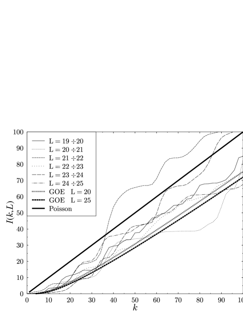
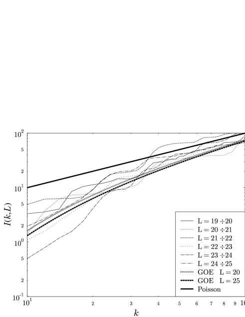
FIG. 9.: The function $I(k,L)$ for the hyperbola billiard. For convenience we present the results on linear-linear and log-log scales.

B The 2D Sinai billiard

Here we considered the 2D Sinai billiard with edge of length $2$ and an inscribed circle of radius $R=0.5$. The billiard was desymmetrized into quarter and POs were computed by Schanz and Smilansky [38]. The database consisted of about 5000 POs in the interval $L<10$ (not including time reversal and $x\leftrightarrow y$ reflection symmetries). Our numerical results of $I(k,L)$ were computed in the interval $7\leq L\leq 10$. We found it very useful to separate the POs into classes according to the number $n$ of their bounces with the circle. The actual justification for this separation into classes is a-posteriori, but following is also an a-priori motivation. Each bounce with the inscribed disc significantly increases (on average) the instability of the orbit. Hence, POs with different $n$’s have in general very different amplitudes. Therefore, if we calculate $C(k,L)$ with the amplitudes $A_{j}$ taken into account, then the relatively few POs with 1–2 bounces dominate and overwhelm the much smaller contributions of the other POs (which are much more numerous). On the other hand, if we ignore $A_{j}$’s (expect sign) and replace them by some average value, then orbits with small number of bounces will be effectively ignored. (This state of affairs is valid when $L$ is relatively small and the $n=1$ class dominates. In general, the important factor is the multiplication of the density $d_{n}(L)$ of orbits with $n$ bounces near length $L$ with the typical amplitude $A_{n}(L)$.) In order to extract as much information as possible, it is imperative to separate the POs into classes according to $n$, such that all of the $A_{j}$ in the same class are of similar magnitude. The numerical results are shown in figure 10. Similarly to the case of the hyperbola billiard PO-correlations are clearly observed, and the general appearance is similar to the predictions of GOE that correspond to the length interval investigated. The numerical dispersion is, however, too large to allow a detailed test of the $L$-dependence.

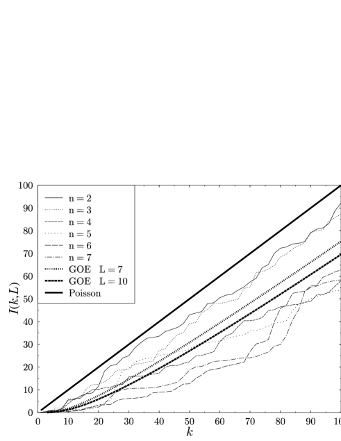
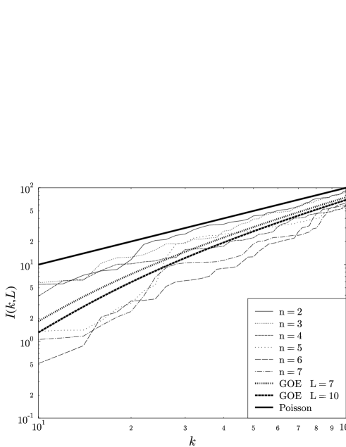
FIG. 10.: The function $I(k,L)$ for the 2D quarter Sinai billiard. POs were considered in the length interval $7\leq L\leq 10$.

The numerical results indeed indicate that the division into classes according to $n$ is very useful as suggested above. It confirms the idea that there are non-trivial correlations between POs within the same class. This information is very valuable in the quest for the classical origin of PO-correlations. We shall exploit it in the case of the 3D Sinai billiard (see below). The existence of inter-class correlations as was shown above does not exclude the possibility of having intra-class correlations, but we did not investigate this issue.

C The 3D Sinai billiard

In this subsection we investigate the classical PO-correlations of the 3D Sinai billiard. The 3D Sinai billiard is the natural extension of the familiar 2D Sinai billiard, and is defined as the free space between a cubic 3-torus and an inscribed sphere. It is presented in figure 11. We consider a torus of edge $1$ and sphere of radius $R=0.2$. The billiard is desymmetrized into its fundamental domain (1/48 of the original billiard). The main reason for investigating this system is that we had an extensive database available that consisted of $7\cdot 10^{6}$ POs (not including time-reversal conjugates). This allows us to perform meaningful statistical checks. The 3D Sinai billiard is plagued with non-generic neutral families of POs (“bouncing-balls”) which were already mentioned in connection with the mixed boundary conditions systems (subsection IV E). As was discussed there, we should resort to the trace formula (4.39) that avoids the bouncing-balls, and takes into account only the generic, isolated and unstable POs. Consequently, the classical spectral density is defined with the coefficients $\tilde{A}_{j}$ rather than with $A_{j}$.

FIG. 11.: The 3D Sinai billiard. Left: original billiard, middle: desymmetrized billiard, right: unfolded billiard.

For a generic billiard system with time reversal symmetry one expects that the quantal form factor will satisfy $K_{qm}\approx K_{GOE}\approx g_{\mbox{eff}}K_{D}(t)$ where $g_{\mbox{eff}}\approx 2$. The similarity $K_{qm}\approx K_{GOE}$ should hold globally while the similarity $K_{qm}\approx g_{\mbox{eff}}K_{D}$ holds for relatively short times. Also for the 3D Sinai billiard with mixed boundary conditions it has been observed [39] that globally $K_{qm}\approx K_{GOE}$, provided that $K_{qm}$ is normalized such that it approaches $1$ for $L\rightarrow\infty$. However, for short times $K_{GOE}<K_{qm}<g_{\mbox{eff}}K_{D}$. The deviation from GOE for short times is a non-generic feature of the system and will not concern us here. The deviation from the diagonal approximation will be discussed in the sequel in terms of classical correlations.

As for the 2D case, we classify the POs according to the number of their bounces $n$ from the inscribed sphere. The a-priori reason is that the amplitudes are very strongly correlated with $n$ (much more than in the 2D case) and the division into the $n$-classes due to this hierarchy is plausible. In figure 12 we present the function $I(k,L)$ for $n=1,2,3$ and various lengths. The numerical results leave no doubt about the existence of classical PO-correlations. All of the data curves are strikingly different from the Poisson (lack of correlations) case. The division into classes turns out to be very useful in revealing very prominent correlations. Closer look at the data shows that the numerical correlations are generally weaker than GOE for low $k$’s ($k\lesssim 30$) and are stronger otherwise. One might interpret this discrepancy as due to a non-generic effect (that prevails at least for low $L$’s), but nevertheless we bear in mind that in the $L$-regime in which we worked the $n=1$ term was dominant, and its correlations are not so different from the universal ones. Also, there is no clear and systematic $L$-dependence. The numerical data exhibit large dispersion that prevents us from concluding anything definite concerning the $L$-dependence. It is therefore useful to examine the correlations for a fixed $L$ and various $n$’s. This is done in figure 13, where we fixed $L=5$ and examined the correlations for $n=1,\ldots,7$. This figure clearly indicates the systematic increase of correlations with increasing $n$.

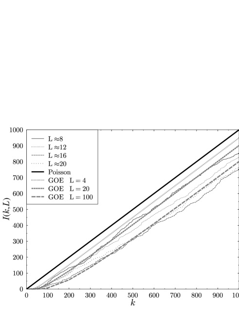
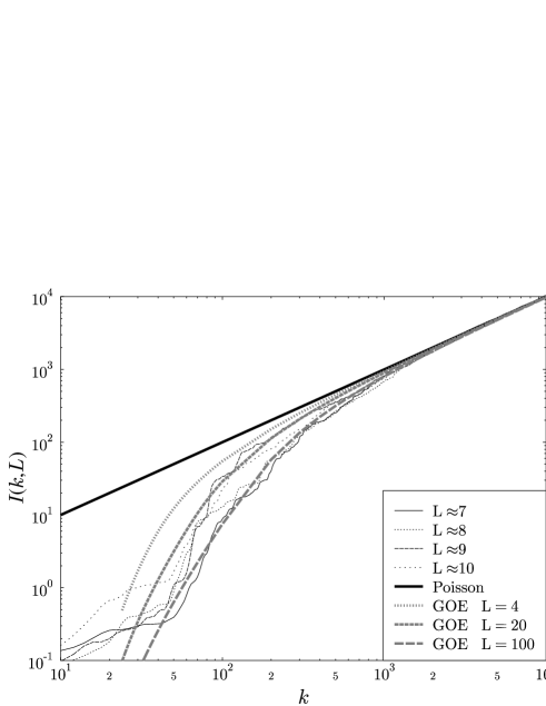
FIG. 12.: The integrated correlation factor $I(k,L)$ for the 3D Sinai billiard with $R=0.2$ (desymmetrized). POs are classified according to their number of bounces from the sphere. Top: $n=1$, middle: $n=2$, bottom: $n=3$. The notation “$L\approx 8$” means a window in $L$ near $L=8$. On the left we present the data in linear scale, and on the right on log-log scale. The GOE predictions are truncated for $k$ smaller than the smallest eigenvalue $k_{1}\approx 23.5$.

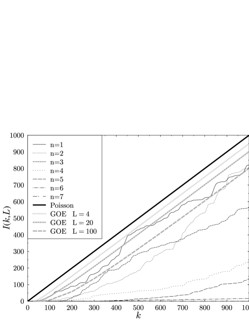
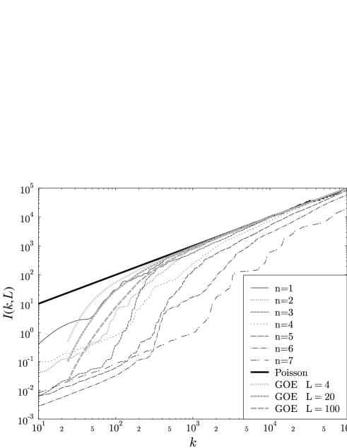
FIG. 13.: The integrated correlation factor $I(k,L)$ for 3D Sinai billiard with $L=5$ fixed and $n$ varied.

To get a hint about the source of the PO-correlations, we have fixed $L=10$ and $n=2$ and varied the radius of the inscribed sphere. The results are shown in figure 14. We clearly observe the growth of the correlations as $R$ decreases. This effect is qualitatively explained by the following argument. Given a PO of the full 3D Sinai billiard (on the torus), it can be described by listing the locations of the centers of the spheres from which it bounces. One should use for this purpose the unfolded representation of the billiard (see figure 11). This list of “addresses” defines the code word $W$ which is known to be unique [41, 51]. This uniqueness property does not hold for the desymmetrized Sinai billiard. Here, the code word $W$ does not determine the PO uniquely. Periodicity is required in the desymmetrized domain, hence one has to determine additionally the symmetry element $\hat{g}$ according to which the PO closes on itself in the unfolded representation. This is illustrated in figure 15. For the 3D Sinai billiard, the symmetry group is $O_{h}$ [42] which contains 48 elements. Therefore, there are up to 48 POs that visit the same spheres in the unfolded domain. We denote this set as $\gamma(W)$. If the radius $R$ is small enough, the lengths of all of the orbits in $\gamma(W)$ will be similar, and the orders of magnitude of their instability amplitudes are expected to be the same. The signs of the amplitudes within $\gamma(W)$ will differ, however, according to the parity of the symmetry element. Hence we expect a better and better cancelations within each $\gamma(W)$ as $R\rightarrow 0$. This qualitatively explains the effect seen in figure 14.

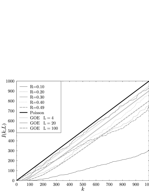
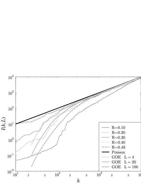
FIG. 14.: The integrated correlation factor $I(k,L)$ for 3D Sinai billiard with $L=10$ and $n=2$ fixed and $R$ varied.

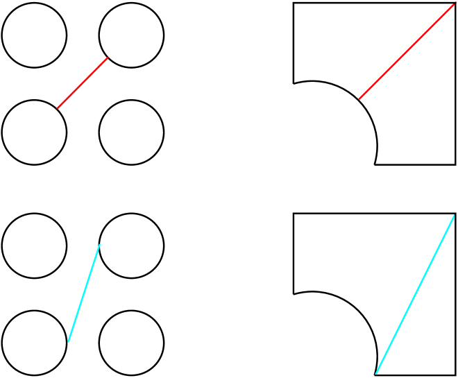
FIG. 15.: Two different POs with the same coding. The POs visit the same discs, but correspond to two different symmetry elements. The illustration is for the 2D Sinai billiard, but the same principle applies also to the 3D Sinai billiard.

To test this argument we performed a numerical experiment, in which we gradually destroyed the possible correlations in a controlled way. The results are displayed in figure 16. Two cases were considered: $R=0.2,L\approx 10,n=2$ and $R=0.2,L\approx 5,n=5$. We first plotted the full correlations in which the coefficients $A_{j}B_{j}$ are taken into account (see (4.39)). As in previous cases, strong classical PO-correlations are observed. We next disregarded the $B_{j}$ factors, and re-calculated $I(k,L)$ using only $A_{j}$’s. As clearly seen from the figure, the changes were minor. Next, we replaced the $A_{j}$’s with their signs $\pm 1$, disregarding their magnitude. Correlations were somewhat diminished, but one can say with full confidence that strong and significant correlations still prevail. This proves, that the coefficients are responsible to part of the correlations, but more importantly, it proves that there are correlations between the actions, regardless of the coefficients. This gives a justification to our point of view taken in the theoretical part, in which we regarded the $A_{j}$’s as “slowly varying”. The following step was to perform a controlled randomization of the $\pm 1$ coefficients between $\gamma(W)$ sets. We picked each set of orbits $\gamma(W)$ and either kept the original signs or reversed all of them. This means, that we kept the relative sign within each $\gamma(W)$. The definite result was that PO-correlations persisted! This proves, that the correlations between POs are largely due to correlations within the sets $\gamma(W)$. To complete the argument, we randomized also the signs within each $\gamma(W)$, and indeed correlations were completely destroyed. The overall conclusion is that we were able to identify the grouping of orbits into sets with the same code word $W$ but with different symmetry $\hat{g}$ as a prominent source of the classical PO-correlations in the 3D Sinai billiard.

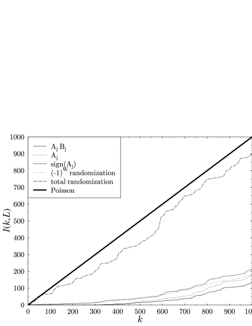
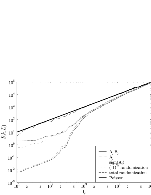
FIG. 16.: Controlled breaking of correlations. See text for details. In both cases $R=0.2$. Upper plots: $L\approx 10,n=2$. Lower plots: $L\approx 5,n=5$.

The above investigation of PO-correlations was purely classical. It is therefore very interesting to enquire whether the quantal levels “feel” the observed classical PO-correlations. To do this, we compared $K_{qm}(k,L)$ (based on the left hand side of (4.39)) to $g_{\mbox{eff}}K_{D}(L)$ (based on the right hand side of the same equation). The quantal from factor $K_{qm}$ was computed from the exact quantal levels and velocities, and $g_{\mbox{eff}}K_{D}(L)$ was computed from the classical PO data (we did not assume any sum rule). The results are shown in figure 17. Note, that we integrated the resulting form factors in $L$ to diminish fluctuations, and started the integration at $L=5$ where the density of POs is already very high. Evidently, the classical diagonal approximation $g_{\mbox{eff}}K_{D}$ is consistently and significantly larger than $K_{qm}$ in the $(k,L)$ regime that we checked. Strong classical non-trivial correlations are therefore needed in order to “bend” $g_{\mbox{eff}}K_{D}$ down to the correct $K_{qm}$. Indeed, in the relevant $(k,L)$ domain, the classical correlation factor $C(k,L)$ for the dominant $n=1$ contribution is $\approx 0.7g_{\mbox{eff}}$ (see figure 12). Quantitatively, if we multiply $g_{\mbox{eff}}K_{D}$ by the numerical factor $0.7$, then we get on the average compliance with the quantum results, as seen in figure 17. Therefore, we have demonstrated a case in which classical correlations are clearly manifest in the quantum mechanical spectral statistics.

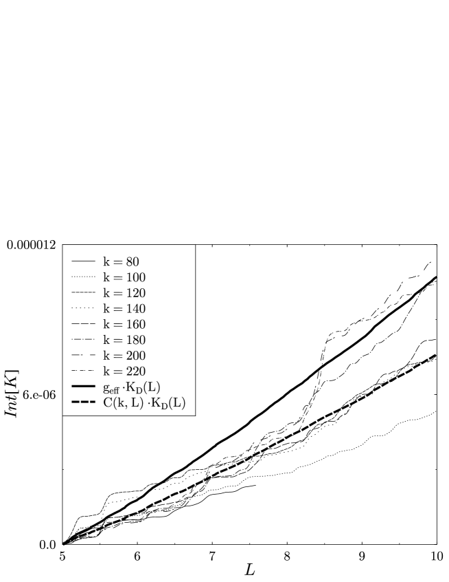
FIG. 17.: Comparison between the quantal and the classical form factors for 3D Sinai billiard with $R=0.2$.

 

Appendices

A Effect of Deformation on PO-s Statistics

Consider a billiard and a particular PO. Assume that the boundary of the billiard in the vicinity of one hitting point is deformed, so that the normal shift is $b$. Assuming no bifurcation, the length of the PO will become $L_{j}\rightarrow L_{j}+\delta_{j}$, where $\delta_{j}=2b\cos(\theta_{j})$. The incidence angle $\theta_{j}$ is measured with respect to the normal direction at the point where the PO hits the deformed surface. In order to prove this result let us define a coordinate $x$ along the boundary (without loss of generality we consider a planar 2D system). The hitting points are $(x_{1},x_{2},...,x_{n})$. The PO constitutes an extremum of the length functional ${\cal L}(x_{1},x_{2},...,x_{n})$, thus $\delta{\cal L}/\delta x_{s}=0$ for the PO. For a deformation $\delta{\cal L}=(\delta{\cal L}/\delta b){\cdot}b+\sum_{s}(\delta{\cal L}/\delta x_{s}){\cdot}(\delta x_{s}/\delta b){\cdot}b=(\delta{\cal L}/\delta b){\cdot}b$. Hence, in order to derive the required result, it is legitimate to fix all the hitting points and to consider merely the length change of the chords due to the deformation. This final step is trivial.

We now wish to consider the effect of general deformation on the two point statistics. Assuming that there are no bifurcations, the new lengths are $L_{j}\rightarrow L_{j}+\delta_{j}$. Treating the differences $y=\delta_{j}{-}\delta_{i}$ as realizations of independent random variables with probability distribution $G(y)$, one obtains $\langle\sum^{\prime}A_{i}^{*}A_{j}\delta(x-(L_{j}{-}L_{i})-(\delta_{j}{-}\delta_{i}))\rangle=\int dyG(y)\langle\sum^{\prime}A_{i}^{*}A_{j}\delta(x-y-(L_{j}{-}L_{i}))\rangle$. The prime implies omission of the diagonal terms $i=j$. It is implicit that the sum is restricted to some $L$-window. From here one easily derive the result $C(k)\rightarrow[1-\tilde{G}(k){\cdot}(1{-}C(k))]$, where $\tilde{G}(k)$ is the FT of $G(y)$.

The case of symmetry breaking due to deformation that preserves family-structure should be treated somewhat differently. Here it is convenient to write the change of length as $L_{j}\rightarrow L_{j}+\delta_{\alpha r}$, where $\alpha$ identifies families of the folded system and $r$ distinguish between families of the unfolded system. Disregarding cross-correlations between families the double sum can be written as $\langle\sum_{\alpha}\sum_{ij}\sum_{rs}A_{i}^{*}A_{j}\delta(x-(L_{j}{-}L_{i})-(\delta_{\alpha r}{-}\delta_{\alpha s}))\rangle$. The $ij$ summation is over POs of the folded system that belong to the $\alpha$ family. This sum can be manipulated as before, note that it is essential to separate the $r\neq s$ from the $r=s$ terms, yielding $\int dy\langle\sum_{ij}\sum_{rs}A_{i}^{*}A_{j}\delta(x-y-(L_{j}{-}L_{i}))\cdot[\delta_{rs}\delta(y)+(1{-}\delta_{rs})G(y)]\rangle=\int dy\langle\sum_{ij}A_{i}^{*}A_{j}\delta(x-y-(L_{j}{-}L_{i}))\cdot g[\delta(y)+(g{-}1)G(y)]\rangle$. From here one easily derive the result $C(k)\rightarrow[1+(g{-}1)\tilde{G}(k)]{\cdot}C_{0}(k)$.

B Diagonal Sums for the Chain Problem

We consider a chain that consists of $N$ cells. The average escape time out of a cell is found as in section V-C, yielding $1/t_{0}=2\times a_{0}^{d_{0}{-}1}/\Omega_{0}$. Here $\Omega_{0}$ is the volume of a single cell, and $a_{0}^{d_{0}{-}1}$ is the cross section of each of the two ‘holes’ that connect the cell to the other cells. Let $x$ be an integer coordinate that identifies the cells, and let $p(x)$ be the probability for finding the particle in the $x$-cell. This probability satisfies the equation

$$\frac{dp(x)}{dt}\ =\ -\frac{1}{2t_{0}}[2p(x)-p(x{-}1)-p(x{+}1)]\ \approx\ -\frac{1}{2t_{0}}\frac{\partial^{2}}{\partial x^{2}}p(x)\ \ \ \ .$$ (B.1)

Above the difference equation is approximated by a diffusion equation. This approximation is valid on time scales such that $p(x)$ is smeared over many cells.

For an open chain of $n$ cells ($n<N$) we solve this equation with the boundary conditions $p(n/2)=p(-n/2)=0$, meaning that there is a zero probability to return once the particle escapes from the endpoints (‘absorption’). We denote by $p(x|x^{\prime})$ the solution, where $x^{\prime}$ is the cell where the particle is initially prepared. In order to solve the diffusion equation one should define an appropriate set of orthonormal functions, which is in the present case:

$$\varphi_{s}(x)\ =\ \left\{\matrix{\sqrt{2}\cos(\pi sx/n)&\ \ \ \mbox{for}\ \ s=1,3,5,...\cr\sqrt{2}\sin(\pi sx/n)&\ \ \ \mbox{for}\ \ s=2,4,6,...}\right.$$ (B.2)

Then we obtain the solution

$$p(x|x^{\prime})\ =\ \sum_{s=1}^{\infty}\mbox{e}^{-(\pi^{2}s^{2}t)/(2n^{2}t_{0})}\ \varphi_{s}(x^{\prime})\varphi_{s}(x)$$ (B.3)

The classical probability to return is simply

$$p_{n}(t)\ =\ \int_{-n/2}^{n/2}p(x|x)dx\ =\ \sum_{s=1}^{\infty}\exp\left(-\frac{\pi^{2}s^{2}t}{2n^{2}t_{0}}\right)\ \ \ .$$ (B.4)

If the chain were closed then $p(x|x^{\prime})\rightarrow 1/n$ for $t\rightarrow\infty$, and consequently one would obtain the asymptotic ergodic result $p_{n}(t)\rightarrow 1$. However, for an open chain the particle will escape eventually via the endpoints-holes, leading to the asymptotic result $p_{n}(t)\rightarrow 0$. Specifically, for very long times $n^{2}t_{0}\ll t$ one obtains $p_{n}(t)\approx\exp(-\pi^{2}t/(2n^{2}t_{0}))$. For intermediate times ($t\ll n^{2}t_{0}$ but still $t_{0}\ll t$), one obtains $p_{n}(t)\approx n/\sqrt{2\pi(t/t_{0})}$. The latter result is not sensitive to the endpoint conditions and is valid also for a closed chain. For short times ($t$ of the order $t_{0}$) the above solution is valid qualitatively but not quantitatively. In particular, for $n=1$ one should obtain the one-cell result $p_{1}(t)=\exp(-t/t_{0})$.

We turn now to the estimate of $K_{n}(t)$ which is the diagonal sum that corresponds to a class of POs that explore $n$ specified cells. For a closed chain there are $N$ classes that correspond to each $n<N$, and one class that correspond to $n=N$. The sum $K_{N}(t)+\sum_{n<N}NK_{n}(t)$ should be equal to $tP_{cl}(t)$. For $t\ll N^{2}t_{0}$ we have the result $P_{cl}(t)=p_{N}(t)=N/\sqrt{2\pi(t/t_{0})}$, and furthermore the first term $K_{N}(t)$ is negligible. For any finite $t$ we may take the limit $N\rightarrow\infty$ thus obtaining the sum-rule

$$\sum_{n=1}^{\infty}K_{n}(t)\ =\ \frac{t}{\sqrt{2\pi(t/t_{0})}}\ \ \ .$$ (B.5)

For an open chain that consists of $n$ cells there are $(n{-}n^{\prime}{+}1)$ classes of POs that explore $n^{\prime}$ cells. Thus we obtain the sum rule

$$\sum_{n^{\prime}=1}^{n}(n{-}n^{\prime}{+}1)K_{n^{\prime}}(t)\ =\ t\cdot p_{n}(t)\ \ \ .$$ (B.6)

The sum rule (B.5) is actually a special case of (B.6), it is obtained by considering finite $t$, taking the limit $n\rightarrow\infty$ and neglecting $(-n^{\prime}+1)$. Using the above sum rules we may obtain an explicit expressions for the functions $K_{n}(t)$.

At this stage it is useful to note the scaling properties of $K_{n}(t)$. Looking on POs of length $t$, the probability for finding a PO that explores $n$ cells should be proportional to $K_{n}(t)$. It is obvious that this probability should depend on the scaled variable $n/\sqrt{t/t_{0}}$. Taking into account the sum-rule (B.5), one obtains the scaling relation

$$K_{n}(t)\ =\ \frac{t_{0}}{\sqrt{2\pi}}f\left(\frac{n}{\sqrt{t/t_{0}}}\right)\ \ \ \ \ .$$ (B.7)

Above, $f(\tau)$ is the scaled probability function. It should have the normalization $1$. Substitution of (B.7) into (B.6), and changing from summation over $n$ to integration over $x=n/\sqrt{t/t_{0}}$ one obtains $\int_{0}^{x}(x{-}x^{\prime})f(x^{\prime})dx^{\prime}=\sqrt{2\pi}\sum_{s=1}^{\infty}\exp(-\pi^{2}s^{2}/(2x^{2}))$. Hence

$$f(x)\ =\ \frac{d^{2}}{dx^{2}}\left[\sqrt{2\pi}\sum_{s=1}^{\infty}\exp\left(-\frac{1}{2x^{2}}(\pi s)^{2}\right)\right]\ =\ \frac{d^{2}}{dx^{2}}F(x)\ \ \ \ \ ,$$ (B.8)

where, by Poisson summation

$$F(x)\ =\ -x+\sqrt{\frac{\pi}{2}}\sum_{s=-\infty}^{\infty}\exp\left(-\frac{1}{2x^{2}}(\pi s)^{2}\right)\ =\ 2x\sum_{r=1}^{\infty}\exp\left(-2x^{2}r^{2}\right)\ \ \ \ \ .$$ (B.9)

The Function $F(x)$ satisfies $F(0)=\sqrt{\pi/2}$ and $F(\infty)=0$ and the corresponding derivatives are $F^{\prime}(0)=-1$ and $F^{\prime}(\infty)=0$. It follows that $\int_{0}^{\infty}f(x)dx=1$ while $\int_{0}^{\infty}xf(x)dx=\sqrt{\pi/2}$. The function $f(x)$ is plotted in Fig.6. It is peaked around $x\sim 1.2$ and it vanishes for either $x\rightarrow 0$ or $x\rightarrow\infty$.

REFERENCES

- [1] To obtain (2.6) one should use the SCTF with replaced by , and multiply both sides by where is the center of the window. Then one should perform a Fourier transform in the variable to the variable .
- [2] The existence of a finite bifurcation-free energy interval requires a further restriction over the periods . This restriction can be realized by using an appropriate windowing procedure.
- [3] H. P. Baltes and E. R. Hilf, Spectra of Finite Systems, Bibliographisches Institut, Mannheim (1996).
- [4] J.P. Keating ”The Riemann Zeta Function and Quantum Chaology”, Proceedings of the International School of Physics ”Enrico Fermi”, Course CXIX, Ed. G. Casati, I. Guarneri and U. Smilansky (North Holland 1993).
- [5] K.G.Andersson and R.B.Melrose, Inventiones math. 41, 197 (1997).
- [6] M.C. Gutzwiller, Chaos in Classical and Quantum Mechanics (Springer-Verlag, New York, 1990).
- [7] The notion of third entropy is explained in [6] p.153 and p.307.
- [8] M. V. Berry and M. Tabor Proc. Roy. Soc. A349 101-123 (1976)
- [9] Ya. G. Sinai in Geometric Aspects of Functional Analysis Lecture Notes in Math. 1469, Springer, Berlin 41-59 (1990)
- [10] P. M. Bleher ibid pp 60-89. and Duke Math. Jour. 74 45-93 (1994).
-
[11]
P. Gaspard and D. Alonso,
Phys. Rev. A 47, R3468 (1993).
D. Alonso and P. Gaspard, CHAOS 3 (4), 601 (1993). - [12] J. H. Hannay and A. M. Ozorio de Almeida, J. Phys. A 17, 3429 (1984).
- [13] T. Harayama and A. Shudo, J. Phys. A: Math. Gen. 25, 4595 (1992).
- [14] M.A. Sepulveda, S. Tomsovic and E.J. Heller, Phys. Rev. Lett. 69, 402 (1992).
- [15] H. Primack and U. Smilansky, Phys. Rev. Lett. 76, 1615 (1996).
- [16] R. Artuso, E. Aurell and P. Cvitanović, Nonlinearity 3, 325 (1990), and references therein.
- [17] M.V. Berry, Proc. R. Soc. London A400, 229 (1985).
-
[18]
E. Doron, U. Smilansky and T. Dittrich,
Physica B179, 1 (1992).
N. Argaman, U. Smilansky and Y. Imry, Phys. Rev. B47, 4440 (1993). -
[19]
N. Argaman, F.M. Dittes, E. Doron,
J.P. Keating, A.Y. Kitaev, M. Sieber and U. Smilansky,
Phys. Rev. Lett. 71, 4326 (1993). - [20] S.Fishman and J.Keating, private communication.
- [21] D. Cohen, ”Periodic Orbits Breaktime and Localization”, chao-dyn/9612014 (1996).
- [22] D. Miller, ”Toward Semiclassical Theory of Quantum Level Correlations of Generic Chaotic Systems” (1997).
-
[23]
A.V. Andreev and B.L. Altshuler,
Phys. Rev. Lett. 75, 902 (1995).
O. Agam, B.L. Altshuler and A.V. Andreev, Phys. Rev. Lett. 75, 4389 (1995). - [24] B.A. Muzykantskii and D.E. Khmelnitskii, JEPT Lett. 62, 76 (1995); Pis‘ma Zh. Eksp. Teor. Fiz. 62, 68 (1995).
- [25] E.B. Bogomolny and J.P. Keating, Phys. Rev. Lett. 77, 1472 (1996).
- [26] R.Scharf and B.Sundaram, Phys. Rev. Lett. 76, 4907 (196).
- [27] T. Dittrich, Phys. Rep. 271, 267 (1996).
- [28] T. Dittrich, B. Mehlig, H. Schanz and U. Smilansky, Chaos Solitons & Fractals 8, 1205 (1997).
-
[29]
B.D. Simons and B.L. Altshuler, Phys. Rev. Lett 70, 4063 (1993).
N. Taniguchi and B.L. Altshuler, Phys. Rev. Lett 71, 4031 (1993). - [30] J.Keating, private communication.
- [31] Z.Rudnik, private communication.
- [32] M. Sieber, H. Primack, U. Smilansky, I. Ussishkin and H. Schanz, J. Phys. A 28, 5041 (1995).
- [33] M. Sieber, U. Smilansky, S. C. Creagh, and R. G. Littlejohn, J. Phys. A 26, 6217 (1993).
- [34] H. Primack and U. Smilansky, Phys. Rev. Lett. 74, 4831 (1995).
- [35] H. Schanz and U. Smilansky, Chaos Solitons and Fractals 5(7), 1289 (1995).
- [36] M. Sieber, PhD thesis, University of Hamburg, DESY preprint 91-030 (1991).
- [37] We thank Martin Sieber for periodic orbit data of the hyperbola billiard.
- [38] We thank Holger Schanz for periodic orbits data of the 2D Sinai billiard.
- [39] Harel Primack, PhD thesis, The Weizmann Institute of Science (1997, in preparation).
- [40] P. Dahlqvist and R. Artuso, preprint, chao-dyn/9601013 (1996).
- [41] L. A. Bunimovich. Chaos 5, 349 (1995).
- [42] M. Tinkham, Group Theory and Quantum Mechanics, McGraw-Hill Book Company (1964).
- [43] P. Dahlqvist, J. Phys. A 28, 4733 (1995).
- [44] T. Kottos and U. Smilansky ”Quantum Chaos on Graphs” (preprint, 1997).
- [45] E. Doron and U. Smilansky, Nonlinearity 5, 1055 (1992).
- [46] F.B. Bogomolny, Nonlinearity 5, 805 (1992).
- [47] M. Tabor, Physica D 6, 195 (1983).
- [48] R. Blümel and U. Smilansky, Phys. Rev. Lett. 64, 241 (1990).
- [49] F. Haake, M. Kus, H.-J. Sommers, H. Schomerus, and K. Zyczkowski, J. Phys. A 29, 3641 (1996).
- [50] U. Smilansky, S. Tomsovic and O. Bohigas, J. Phys. A 25, 3261 (1992).
- [51] H. Schanz, PhD dissertation, Humboldt-Universitat zu Berlin (1996).