Probability density and scaling exponents of the moments of longitudinal velocity difference in strong turbulence

${\bf Abstract}.$

We consider a few cases of homogeneous and isotropic turbulence differing by the mechanisms of turbulence generation. The advective terms in the Navier-Stokes and Burgers equations are similar. It is proposed that the longitudinal structure functions $S_{n}(r)$ in homogeneous and isotropic three- dimensional turbulence are governed by a one-dimensional equation of motion, resembling the 1D-Burgers equation, with the strongly non-local pressure contributions accounted for by galilean-invariance-breaking terms. The resulting equations, not involving parameters taken from experimental data, give both scaling exponents and amplitudes of the structure functions in an excellent agreement with experimental data. The derived probability density function $P(\Delta u,r)\neq P(-\Delta u,r)$ but $P(\Delta u,r)=P(-\Delta u,-r)$, in accord with the symmetry properties of the Navier-Stokes equations. With decrease of the displacement $r$, the probability density, which cannot be represented in a scale-invariant form, shows smooth variation from the gaussian at the large scales to close-to-exponential function, thus demonstrating onset of small-scale intermittency. It is shown that accounting for the sub-dominant contributions to the structure functions $S_{n}(r)\propto r^{\xi_{n}}$ is crucial for derivation of the amplitudes of the moments of velocity difference.

Introduction
Intermittency of turbulence, not contained in the Kolmogorov theory, is one of the most intriguing and mysterious phenomena of continuum mechanics. Experimentally detected in the early sixties, this feature of high Reynolds number turbulent flows still remains a major challenge to turbulence theory. Landau’s 1942 remark [1] that the large- scale fluctuations of turbulence production in the energy-containing range can invalidate the Kolmogorov theory was one of the motivations for construction of various “cascade” models attempting to explain this phenomenon, manifested in the anomalous scaling of the structure functions $S_{n}(r)=<(u(x+r)-u(x))^{n}>\equiv<U^{n}>\propto A_{n}r^{\xi_{n}}$ with the exponents $\xi_{n}\neq n/3$. The first model of this kind was proposed by Kolmogorov himself in 1962 [2]. Recently, some important analytic advances, leading to evaluation of both scaling exponents $\xi_{n}$ and the amplitudes $A_{n}$ were made for the problems of the passive scalar, advected by a random velocity field and the random-force-driven Burgers turbulence [3]-[7]. First, it was proposed by Kraichnan [3] that scalar structure functions $<(T(x)-T(x+r))^{2n}>$ can be solutions of homogeneous differential equations , thus leading to the non-trivial values of the exponents $\xi_{n}$ which could not be found from dimensional considerations. Then, Gawedzki and Kupiainen [4], Chertkov et. al. [5]-[6] and Shraiman and Siggia [7] showed that, indeed, it was the zero modes which were responsible for the anomalous scaling in some limiting cases of the passive scalar problem. Similar results were arrived at in many of the following studies [8]-[10].

Polyakov’s theory of the large-scale-random-force-driven Burgers turbulence [11] was based on the assumption that weak small-scale velocity fluctuations ($|u(x+r)-u(x)|<<u_{rms}$ and $r<<L$, where $L$ is the the energy input- scale), obey the galilean invariant dynamic equations, meaning that the integral scale and the random-force- induced single-point $u_{rms}$ cannot enter the resulting expression for the probability density having the scale-invariant form:

$$P(U,r)\approx\frac{1}{r}F(\frac{U}{r})$$

When $U\geq u_{rms}$ galilean invariance (GI), even of the small-scale dynamics can be violated and the PDF scales with $U/u_{rms}$, leading to saturation of the scaling exponents $\xi_{n}=1$ for $n>n_{c}=1$. This general feature of Burgers turbulence was confirmed by numerical experiments in which turbulence was generated by different random forces generating various scaling exponents $\xi_{n\leq n_{c}}$ [12]-[14]. It was shown in Ref. [12]-[14] that the value of the critical moment number $n_{c}$ depended on the forcing function spectrum. Still, at $n>n_{c}$ all $S_{n}\propto r$ indicating that decorrelation introduced by the noise was too weak to prevent the shock formation. Recently Chertkov et. al. [15] obtained a similar structure of the theory considering a one-dimensional problem of a passive scalar advected by a random velocity field. In the limit $r\rightarrow 0$ their PDF

$$P(U,r)\propto\frac{1}{r}\frac{e^{-\frac{U^{2}}{u^{2}_{rms}}}}{U^{2}+r^{2}}$$

where, to simplify notation, we have set the values of all numerical constants equal to unity. Similar result was also obtained in the work on the large-scale- driven Burgers turbulence in when space dimensionality $D\rightarrow\infty$ by Bouchuod et. al. [16].

Polyakov’s idea [11] about the role of violation of galilean invariance in generation of anomalous scaling resonates with Landau’s remark about important influence of the large-scale fluctuations on the small-scale dynamics [1]. In this paper we will attempt to combine the zero-mode and the GI-breakdown ideologies to derive equations governing the probability density function of the longitudinal velocity differences in strong turbulence. We would like to reiterate that two measurements in the same turbulent flow performed in the laboratory and in the moving frame of reference (train or ship) must give the same answers. The “violation of galilean invariance” is understood hereafter only in a limited Polyakov’s sense as a possibility of $u_{rms}$ entering the probability density of velocity difference. It will be shown that the details of the large-scale turbulence production mechanism are important, leading to the non-universality of probability density function (PDF) of velocity difference. The results will be compared with experimental data.

Formulation of the problem
Turbulence in Nature results from hydrodynamic instabilities of various laminar low-Reynolds-number flows. The transition phenomena are is not universal, depending on geometry, external fields etc. and, at the present time, cannot be accounted for by turbulence theory. Hoping for some universality of the small-scale velocity fluctuations in the inertial range, it is customary to develop a theory of turbulence, driven at the large scales by some terms in the Navier-Stokes equations, one can treat theoretically. Usually, these large-scale forcing terms are assumed to be irrelevant in the inertial range. Below we discuss three models corresponding to different mechanisms of turbulence generation. First, let us consider the Navier-Stokes equations on an infinite domain:

$${\bf v}_{t}+{\bf v\cdot\nabla v}={\bf f}-{\bf\nabla}p+\nu\nabla^{2}{\bf v}$$

$${\bf\nabla\cdot v}=0$$

The gaussian large-scale forcing ${\bf f}$ is defined by the two-point correlation function

$$<f_{i}({\bf x},t)f_{j}({\bf x^{\prime}},t^{\prime})>=P_{ij}\kappa(|{\bf x-x^{\prime}}|)\delta(t-t^{\prime})$$

where the projection operator $P_{ij}$ ensures the incompressibility of the solution. The force is assumed acting in the interval of wave-numbers $1/\Omega^{\frac{1}{3}}<<k_{0}\approx 1/L>>k_{d}$ where $\Omega\rightarrow\infty$ and $\eta=1/k_{d}$ are the volume of the system and dissipation scale, respectively. In other words, the forcing spectrum is assumed to decrease very rapidly outside the interval $k\approx k_{0}$. In the limit $k<<k_{0}$ the system is in thermodynamic equilibrium and is described by the gaussian statistics and energy spectrum $E(k)\propto k^{2}$ [17]. Thus, the order of the limits is: first we set the large value of $k_{0}$ and then $\nu\rightarrow 0$, so that $k_{d}/k_{0}\rightarrow\infty$.

In the case of the $\delta$-correlated forcing function (3) the source-related contribution to the equation for the two-point correlation function can be written in a very simple way:

$$W=<v_{i}(x,t)f_{i}(x^{\prime},t)>\propto\kappa(|x-x^{\prime}|)$$

2. Often, in the real- life experimental situations, when turbulence is generated in the vicinity of the boundaries (wall flows), nozzles (jets), bodies (wakes) and later on transported into the bulk of the flow where the measurements take place, the model (1)-(3) is not valid. In this case a better description is given by the initial value problem, taking into account the turbulence decay during this delay time. This will be also discussed in what follows.

3. In the third class of the flows turbulence is produced by a large-scale shear. Then, introducing the so called Reynolds decomposition

$${\bf U=V+v}$$

where ${\bf v}$ ($<{\bf v}>=0$) is the fluctuation from the time-independent mean velocity $<{\bf U}>\equiv{\bf V}$, the equation for velocity fluctuations ${\bf v}$ is given by (1) with ${\bf f=0}$ and the turbulence production term in the right side [1]:

$${\bf(v\cdot\nabla)V}$$

The force-free Navier-Stokes equations are invariant under rotations, space-time translations, parity and scaling transformations. They are also invariant under galilean transformations ${\bf x}\rightarrow{\bf x+Vt}$ and ${\bf v}\rightarrow{\bf v+V}$ where ${\bf V}$ is the constant velocity vector of the moving frame. Boundary conditions and forcing can violate some or all of the symmetries of the equations (1). It is, however, usually assumed that in the high Reynolds number flows with $\nu\rightarrow 0$ all symmetries of the Navier-Stokes (even Euler) equations are restored in the limit $r\rightarrow 0$ and $r>>\eta$ where $\eta$ is the dissipation scale where the viscous effects become important. This means, among other consequences, that in this limit the root-mean square velocity fluctuations $u_{rms}=\sqrt{<}{v^{2}>}$, not invariant under the constant shift, cannot enter the relations describing moments of velocity differences. If all this is correct, then the effective equations for the inertial-range velocity correlation functions must have the symmetries of the original Euler equations. For many years this assumption was the basis of all turbulence theories. Based on the recent understanding of Burgers turbulence [11]-[14], some of the constraints on the allowed turbulence theories will be relaxed in what follows.

We are interested in the multi-point velocity correlation functions:

$$C_{n}({\bf x_{1},x_{2},....x_{n}})=<v_{i1}({\bf x_{1}})v_{i2}({\bf x_{2}})....v_{in}({\bf x_{n}})>$$

and longitudinal structure functions:

$$S_{n}(r)=<((u(x+r)-u(x))^{n}>\equiv<(\Delta u)^{n}>$$

where $u(x)$ is the $x$-component of the three-dimensional velocity field and $r$ is the displacement in the direction of the $x$ axis.

In 1941 Kolmogorov, considering decaying turbulence, derived an equation for $S_{3}(r)$ valid when $r\rightarrow 0$:

$$\frac{1}{r^{4}}\frac{\partial r^{4}~{}S_{3}(r)}{\partial r}=-4{\cal E}+\frac{6\nu}{r^{4}}\frac{\partial^{2}S_{2}(r)}{\partial r^{2}}$$

leading to the famous Kolmogorov $\frac{4}{5}$-law: in the limit $\nu\rightarrow 0$ and at $L>>r>>\eta$ where $\eta$ is the dissipation scale of turbulence defined as:

$$\nu S_{rr}(\eta)=O(1)$$

The third-order structure function in the inertial range $L>>r>>\eta$ is given by a $4/5$ law::

$$S_{3}(r)=-\frac{4}{5}{\cal E}r$$

In fact, the expression (4) is an approximation, neglecting small contributions from time-derivatives and source functions, valid in the limit $r\rightarrow 0$. In general, it must be modified to include the forcing function:

$$S_{3}(r)=-\frac{4}{5}{\cal E}r+O(r\overline{(\Delta u)(\Delta f)})$$

We can see that for a white-in-time large- scale forcing function $\kappa(r)=\kappa(0)-\gamma r^{2}$, the sub-leading contribution to Kolmogorov $4/5$-law in the inertial range $r\rightarrow 0$ is $O(r^{3})$. In a more general situation evaluation of the correction is not so simple.

In case of decaying turbulence the sub-leading contribution to (5) is :

$$O(r\frac{\partial S_{2}(r)}{\partial t})$$

while when turbulence is produced by the large-scale shear, it is somewhat different [18]:

$$O({\bf r\frac{\partial V}{\partial x}}S_{2}(r))$$

When $r$ is small, these terms can be neglected. However, as will be shown below, they must be accounted for since the procedure of evaluation of the probability density $P(\Delta u,r)$ involves matching of the inertial range and large-scale solutions.

Derivation of (4)-(6) is based on the fact that due to the incompressibility condition, all transverse correlation functions can be expressed in terms of the longitudinal ones leading to the closed equations. One can say that in a very limited sense the procedure projects the original three-dimensional problem onto a one-dimensional one. Regretfully, due to the coupling between different components of the velocity field, caused by the pressure terms, we cannot rigorously derive similar expressions for the high-order moments $S_{n}(r)$. The second difficulty is in the presence of the dissipation anomaly (see below). Still, we can attempt to use some general features of the equations of motion and derive the scaling properties and general form of the probability density function $P(\Delta u,r)$.

Equations for the probability density
One can introduce a generating function

$$Z=<e^{\sum_{i}\lambda_{i}\cdot{\bf v(x_{i})}}>$$

where the vectors ${\bf x_{i}}$ define positions of the points denoted by the numbers $1<i<N$. Using the incompressibility condition, the equation for $Z$ can be formally written:

$$\frac{\partial Z}{\partial t}+\frac{\partial^{2}Z}{\partial\lambda_{i,\gamma}\partial x_{i,\gamma}}=I_{f}+I_{p}+D$$

where $I_{f}$, $I_{p}$ and $D$ are related to the forcing, pressure and dissipation contributions to the Navier-Stokes equation (see below). Although the advection contributions are accurately accounted for in this equation, it is not closed due to the pressure and dissipation terms. The latter can be treated using Polyakov’s operator product expansion ideas [11], while the former presents an additional difficulty to be dealt with. In what follows we will be mainly interested in the moments of the two-point velocity differences which in homogeneous and isotropic turbulence can depend only on the absolute values of two vectors (velocity difference ${\bf v(x^{\prime})-v(x)}$ and displacement ${\bf r\equiv x^{\prime}-x}$) and the angle $\theta$ between them with $\theta=\pi/2$ and $\theta=0$ corresponding to transverse and longitudinal structure functions, respectively. In spherical coordinates the explicitly written advective terms in the equation (7) involve

$$O(\frac{\partial^{2}Z}{\partial\lambda\partial r});~{}~{}O(\frac{1}{r}\frac{\partial Z}{\partial\lambda});~{}~{}O(\frac{1}{\lambda}\frac{\partial Z}{\partial r});~{}~{}O(\frac{Z}{\lambda r})$$

and various trigonometric functions and angular differentiations. The theory of the longitudinal structure functions, presented below, is based on the assumption, correct for the third order moment $S_{3}(r)$ (see (4)), that the angular dependence can be accounted for in a simple way and, as a consequence, there exist an equation for $\theta=0$. This assumption is supported by the following observations. It is easy to show that in the inertial range the second-order structure function

$$S_{2}(r,\theta)=\frac{2+\xi_{2}}{2}D_{LL}(r)(1-\frac{\xi_{2}}{2+\xi_{2}}cos^{2}(\theta))$$

with $D_{LL}(r)=<(u(x)-u(x+r))^{2}>$. More involved relation can be written for the fourth-order moment [16]:

$$S_{4}(r,\theta)=D_{LLLL}(r)cos^{4}(\theta)-3D_{LLNN}(r)sin^{2}(2\theta)+D_{NNNN}(r)sin^{2}(\theta)$$

where $D_{LLNN}=<(v(x)-v(x+r))^{2}(u(x)-u(x+r))^{2}>$ and $v$ and $u$ are the components of the velocity field perpendicular and parallel to the $x$-axis, respectively. As one can easily deduce from the angular dependence, the functions $D_{LLLL}(r)$ and $D_{NNNN}(r)$ denote longitudinal and transverse structure functions, respectively. In the limit $\theta\rightarrow 0$

$$S_{4}(r,\theta)\approx D_{LLLL}(r)cos^{4}(\theta)+O(\theta^{2})$$

rapidly approaching $S_{4}(r,\theta=0)=D_{LLLL}(r)\equiv S_{4}(r)$. Based on the above expressions, we conclude that, as in the theory of multidimensional Burgers turbulence [16], where the probability density of velocity difference can be represented as: $P(U,r,\theta)\approx P(U,rcos(\theta))$, here in the limit $\theta\rightarrow 0$ the mixing of the longitudinal and transverse correlation functions is very weak ($O(\theta^{2})$). As a consequence, we assume that the closed equation for the probability density of longitudinal velocity differences exist. Generalization of the theory to the case of an arbitrary (not small) angle $\theta$ is the subject of an ongoing study.
We select $N$ points ${\bf x_{i}}$ with $0<i<N$ on the $x$-axis and introduce the longitudinal generating function for the $N$-point correlation function:

$$Z_{N}=<e^{\lambda_{i}u(x_{i})}>$$

where $\lambda_{j}=ik_{j}$. The equation of motion for $Z_{N}$ can be formally derived (we neglect the subscript $N$ in what follows):

$$Z_{t}=\sum_{j}\lambda_{j}<e^{\lambda_{i}u(x_{i})}u_{t}(x_{j})>$$

Substituting the N-S equations into this relation gives:

$$Z_{t}=\sum_{j}\lambda_{j}<e^{\lambda_{i}u(x_{i})}[-u(x_{j})\frac{\partial u(x_{j})}{\partial x_{j}}+f_{x}(x_{j})]>+I_{T}+I_{p}+D$$

where $f_{x}(x_{j})$ is the $x$-component of the forcing, $x_{j}$ is the coordinate of the $j^{th}$ point and $\frac{\partial}{\partial x_{j}}$ is the partial derivative in the $x$ direction only. The summation in the expression (10) is over the positions $x_{j}$ and over the Greek subscripts $\alpha=1;~{}2$ denoting the components of the velocity field in the directions perpendicular to the $x$-axis. The life-threatening terms in (10) are:

$$I_{T}=\sum_{j}\lambda_{j}<e^{\lambda_{i}u(x_{i})}[-v_{\alpha}(x_{j})\frac{\partial u(x_{j})}{\partial x_{\alpha j}}]>$$

$$I_{p}=-\sum_{j}\lambda_{j}<e^{\lambda_{i}u(x_{i})}\frac{\partial p(x_{j})}{\partial x_{j}}>$$

and

$$D=\nu\sum_{j}\lambda_{j}<e^{\lambda_{i}u(x_{i})}\frac{\partial^{2}u(x_{j})}{\partial x_{j}^{2}}>$$

The theoretical and numerical work [16] on the multi-dimensional Burgers equation led to the probability density and moments of velocity difference basically independent on the space dimensionality: the moments $S_{n\leq 1}(r)\propto r^{n}$ while $S_{n\geq 1}\propto r$. This is an indication that the shock production, dominated by the longitudinal components of the nonlinearity $u_{i}\partial_{i}u_{i}$ (no summation over the subscript $i$), prevails over the processes coming from the mixed terms of the kind $u_{j}\partial_{j}u_{i}$ which can be neglected. In other words the multi-dimensional Burgers equation is well approximated by the system of weakly interacting 1D-equations acting along various coordinate axis. It is clear that geometry of the objects generated by this system is very complex. The recent paper by Gurarie and Migdal [16], dealing with the two- and three-dimensional Burgers turbulence, introduced an angle $\theta$ between velocity difference and displacement vectors ${\bf v(x+r)-v(x)}$ and ${\bf r}$, respectively, and using the instanton formulation, derived an expression for the generating function (see below) $Z_{2}$ in the form $Z_{2}\propto exp((\lambda r)^{\gamma}f(cos\theta))$ with $\gamma=3/2$ independently on space dimensionality and $\lambda=|{\bf\lambda}|$ and $r=|{\bf r}|$. The calculated function $f(cos(\theta))$ ensured correct angular dependence of multi-dimensional structure functions. When $\theta=0$, the derived expression basically recovered the one-dimensional Polyakov’s result. This result tells us that it is the projection of the velocity field on the direction of the displacement vector ${\bf r}$ that produces dynamically significant contribution to the multi-dimensional structure functions and that the longitudinal structure functions in three-dimensional Burgers turbulence are close to those in the 1D-turbulence. Indeed, numerical simulations [16] of the three-dimensional Burgers turbulence revealed very complex velocity field with the structure functions $S_{n}(r)$ very close to the ones, previously obtained in one-dimensional simulations. The possible smallness of interaction between different components of the advective terms is only part of the story. The pressure contribution $I_{p}$ leads to effective energy redistribution between components of the velocity field and plays an important part in the Navier-Stokes dynamics. The pressure effects are nonlocal, instantaneously transporting information between different, even very remote, parts of the flow. That is why the effects coming from the boundary conditions and large scale forces cannot be neglected even in description of the small-scale phenomena. The possible spontaneous breakdown of galilean invariance is the central assumption of this work.

The equation (10) can be rewritten as:

$$Z_{t}=\sum\lambda_{i}\lambda_{j}\kappa(|x_{i}-x_{j}|)Z-\sum_{j}[\frac{\partial^{2}Z}{\partial\lambda_{j}\partial x_{j}}-\frac{1}{\lambda_{j}}\frac{\partial Z}{\partial x_{j}}]+I_{T}+I_{p}+D$$

where the large-scale gaussian random force is defined in the limit $r\rightarrow 0$ by the correlation function: $\kappa(r)=\kappa(0)-\gamma r^{2}$. Approaching the integral scale $L$ the force correlation function $\kappa(r)$ rapidly goes to zero. We will see that the equation for the probability density of the velocity difference $P(U,r)$ where $U=u(x+r)-u(x)$ contains the combination $\kappa(0)-\kappa(r)$ which is large at the large scales $r\rightarrow L$. That is why the large-scale dynamics, dominated by the forcing term, show close to gaussian behavior of at least the first few moments $S_{n}$.

Evaluation of $I_{T}$, $I_{p}$ and $D$ in (14) is a difficult problem and we have to make some assumptions. It is seen from the definition of the generating function $Z_{N}$ that when two points merge, i.e. $x_{i}\rightarrow x_{j}$ the $N$-point generating function becomes the $N-1$-point generating function with $\lambda=\lambda_{i}+\lambda_{j}$. This means that if, for example, the equation for $Z_{2}$ contains the two-point sum:

$$\varphi(\lambda_{1},u(x_{1}),x_{1},\frac{\partial}{\partial x_{1}})Z_{2}+\varphi(\lambda_{2},u(x_{2}),x_{2},\frac{\partial}{\partial x_{2}})Z_{2}\rightarrow a(\lambda,y)\varphi(\lambda,u(x_{1}),x_{1},\frac{\partial}{\partial x_{1}})Z_{1}$$

Here $\varphi$ depends on the structure of the equation of motion and $y=|x_{i}-x_{j}|\rightarrow 0$. We assume that in this limit the unknown function $a(\lambda,0)$ is finite. Not all functions $\varphi$ satisfy this equation. For example: $\varphi=\lambda$ and $\varphi=\lambda\frac{\partial}{\partial\lambda}$, do. The functions $\varphi$ can also include space derivatives. Combined with the general symmetry properties of (14) we can narrow the class of possible solutions and derive equation for the probability density. It follows from the Navier-Stokes equations that the theory must be invariant under transformation: $\lambda\rightarrow-\lambda$ and $x_{j}\rightarrow-x_{j}$. In what follows we will adopt Polyakov’s result that the main effect of the longitudinal part of the dissipation term $D$ is a renormalization of the coefficient in front of the $O(1/\lambda_{j})$ terms in the right side of (14). Based on the above considerations, we can write two models for the $N$-point generation function, corresponding to the different mechanisms of turbulence production introduced above (see below):

$$Z_{t}=\sum\lambda_{i}\lambda_{j}K(|x_{i}-x_{j}|)Z-\sum_{j}[\frac{\partial^{2}Z}{\partial\lambda_{j}\partial x_{j}}-\frac{b}{\lambda_{j}}\frac{\partial Z}{\partial x_{j}}]+C\sum\lambda_{j}\frac{\partial}{\partial\lambda_{j}}Z+I_{T}+I_{p}+D^{\prime}$$

for the cases 2 and 3 and

$$Z_{t}=\sum\lambda_{i}\lambda_{j}\kappa(|x_{i}-x_{j}|)Z-\sum_{j}[\frac{\partial^{2}Z}{\partial\lambda_{j}\partial x_{j}}-\frac{b}{\lambda_{j}}\frac{\partial Z}{\partial x_{j}}]+I_{T}+I_{p}+D^{\prime}$$

to describe turbulence generated by the white-in-time forcing (3). Here $D^{\prime}$ involves only “transverse” components of the $D$-term defined below. The $O(\lambda\frac{\partial Z}{\partial\lambda})$- term in (15) comes from the $O({\bf v})$ turbulence production, while $K(r)=K(0)-\beta r^{2}$, leading to the negligibly small $O(r^{2})$ sub-leading contributions to the velocity difference structure functions, ensures the close-to-gaussian single-point probability density. The equations (15)-(16) violate neither “fusion rules” introduced above nor general symmetries of the Navier-Stokes equations. By dimensionality, the coefficient $C/\kappa(0)=O(1/u_{rms}^{2})$. The $O(\kappa(r))$ term in the equation (16), stems from the forcing function (3). Below we will discuss the two cases in detail.

If one is interested in a single-point probability density, the equation (15) is to be solved for all $x_{j}=x$ and $\lambda=\sum_{j}\lambda_{j}$. All space derivatives disappear due to homogeneity of turbulence and we have an expected result [17]:

$$P(u)=\sqrt{\frac{2}{\pi}}e^{-\frac{u^{2}}{2u^{2}_{rms}}}$$

This fixes the value of the coefficient $C$. Thus, the equation (15) yields gaussian distribution of the single-point velocity field. This result will be used below as a matching condition for the probability density $P(U,r)$ in the large-scale limit $r\rightarrow L$. The experimentally observed single-point probability density $P(u)$ is very close to but not equal to gaussian deviating from it at the large values of velocity fluctuations $u>>u_{rms}$. The theory, developed here, is applicable to any expression for $P(u)$, not only to the gaussian. Still, the gaussian, which will be used below to compare the theoretical predictions with the data, is a very good approximation.

We need an equation for the the generating function $Z_{2}$ with $\lambda_{1}+\lambda_{2}=0$ giving:

$$Z_{2}(\lambda,r)=<e^{\lambda(u(x+r)-u(x))}\equiv<e^{\lambda U}>$$

In a statistically steady state:

$$2\frac{\partial^{2}Z_{2}}{\partial\lambda\partial r}-\frac{2b}{\lambda}\frac{\partial Z_{2}}{\partial r}=\lambda^{2}(K(0)-K(|x_{i}-x_{j}|))Z_{2}+I_{T}+I_{p}+D^{\prime}-\frac{u_{rms}}{L}\lambda\frac{\partial Z_{2}}{\partial\lambda}$$

Where

$$I_{T}=\lambda<[v_{\alpha}(x_{2})\partial_{x_{2},\alpha}u(x_{2})-v_{\alpha}(x_{1})\partial_{x_{1},\alpha}u(x_{1})]e^{\lambda(u(2)-u(1))}>\equiv\lambda<i_{T}e^{\lambda U}>$$

$$I_{p}=<\lambda[\frac{\partial p(x_{2})}{\partial x_{2}}-\frac{\partial p(x_{1})}{\partial x_{1}}]e^{\lambda(u(2)-u(1))}>\equiv\lambda<i_{p}e^{\lambda U}>$$

and

$$D^{\prime}=\lambda\nu<[\partial^{2}_{x_{2}\alpha}u({\bf x_{2}})-\partial^{2}_{x_{1}\alpha}u({\bf x_{1}})]e^{\lambda(u(2)-u(1))}>\equiv\lambda<d^{\prime}e^{\lambda U}>$$

The point merging in $I_{T}$ and $I_{p}$ must be regular while the same procedure in the dissipation term $D^{\prime}$ involves divergences which are cancelled by viscosity $\nu\rightarrow 0$. As was pointed out in [11] the longitudinal, $O(\partial_{x}^{2}u({\bf x}))$, components of the $D$-term result in the renormalization of the coefficient in front of the $O(1/\lambda)$ - contribution to the right side of (14). We are still left with the remaining $O(\partial^{2}_{\alpha}u({\bf x}))$ - piece of the dissipation anomaly, pressure terms $I_{p}$ and the $I_{T}$ - contributions, mixing all components of the velocity field. Having in mind general fusion rules, considered above, and the fact that the equation is invariant under transformation $\lambda\rightarrow-\lambda$ and $r\rightarrow-r$ we, not being concerned with preservation of galilean invariance, write the equation for $Z_{2}$ corresponding to (15):

$$\frac{\partial^{2}Z_{2}}{\partial\lambda\partial r}-\frac{B^{0}}{\lambda}\frac{\partial Z_{2}}{\partial r}=\frac{A}{r}\frac{\partial Z_{2}}{\partial\lambda}-\frac{u_{rms}}{L}\lambda\frac{\partial Z_{2}}{\partial\lambda}$$

The equation (20) includes the derived above expression for the coefficient $C$ and the unknown parameters $B^{o}$ and $A$ to be determined from the theory. The characteristic time in (20) $T\approx L/u_{rms}=O(1)$ is independent on the displacement $r$. A natural generalization of this model is (20) with the last term in the right side:

$$\frac{1}{T(r)}\lambda\frac{\partial Z_{2}}{\partial\lambda}$$

with $T(r)\propto r^{\xi_{\tau}}$ with the exponent $\xi_{\tau}$ depending on the physics of the problem. In Kolomogorov turbulence $\xi_{\tau}\approx 2/3$.

The model corresponding to (16) is:

$$\frac{\partial^{2}Z_{2}}{\partial\lambda\partial r}-\frac{B^{0}}{\lambda}\frac{\partial Z_{2}}{\partial r}=\frac{A}{r}\frac{\partial Z_{2}}{\partial\lambda}+\gamma r^{2}\lambda^{2}Z$$

where the $O(r^{2})$- contribution is to be kept. The equations (20)-(21) are based on the assumption that the dynamic role of the pressure and dissipation terms is in the renormalization of the coefficients in front of the already- present advective contributions (8) to the equation (7). Similar assumption was fruitful in the theory of Burgers turbulence [11]. Except for the last terms in the right side, these equations are the same as the one in Polyakov’s theory of Burgers turbulence with the $B^{o}$ - term simply renormalizing part of the advection effects, present in the original equations. The meaning of the $A$-term will be discussed in detail below. It will be shown that it is not only responsible for prevention of the shock formation but it also makes the weak ($|U|<<u_{rms}$ ) structures of the Navier-Stokes dynamics much stronger than their counterparts of Burgers turbulence. It is clear that due to homogeneity of turbulence, all space derivatives and related to them $A$-contributions go to zero when $r\geq L$ . In the one-dimensional case the dissipation anomaly $D$, discussed in detail by Polyakov, leads only to a relatively small modification of a corresponding coefficient . It will be shown that in case of three-dimensional turbulence $B^{o}\approx-20$, part of which is to be attributed to a large pressure effects preventing the shock formation. In the resulting dynamic equations (20)-(21) the contributions from $D$ and $I_{p}$ are mixed and the origins of each term, hidden in numerical values of the coefficients $b$, $B^{o}$ and $A$, are not easy to establish. The equation (20), explicitly involving the single-point $u_{rms}$ is suited for description of the generating function in both $r\rightarrow 0$ and $r\rightarrow L$ limits. In the inertial range, where the displacement $r$ is small, the $O(u_{rms})$ and the forcing contributions can be neglected. They are important, providing the large-scale gaussian matching constraint, needed for determination of the amplitudes of the structure functions $S_{n}$. Thus, the equations (20)-(21), describing the correlation functions in the inertial range, differ by the last in the right side terms reflecting the details of the large-scale turbulence generation processes. It will be shown below that this difference is responsible for non-universality of the probability density function of velocity difference.

In the limit $r\rightarrow 0$ the equation for the probability density is derived from (20)-(21) readily:

$$-\frac{\partial}{\partial U}U\frac{\partial P}{\partial r}-B^{o}\frac{\partial P}{\partial r}=-\frac{A}{r}\frac{\partial}{\partial U}U~{}P+\frac{u_{rms}}{L}\frac{\partial^{2}}{\partial U^{2}}UP$$

$$-\frac{\partial}{\partial U}U\frac{\partial P}{\partial r}-B^{o}\frac{\partial P}{\partial r}=-\frac{A}{r}\frac{\partial}{\partial U}U~{}P-\gamma r^{2}\frac{\partial^{3}Z}{\partial U^{3}}$$

Properties of the solution
Multiplying (22) by $U^{n}$ and assuming existence of all moments leads to:

$$\frac{\partial S_{n}}{\partial r}=\frac{An}{n+B}\frac{S_{n}}{r}+\frac{u_{rms}}{L}\frac{n(n-1)}{n+B}S_{n-1}(r)$$

where $B=-B^{o}>0$. The equation (24) is to be solved under the constraint (4) which is the result of the energy conservation inherent to the Navier-Stokes equations. This is the consequence of the renormalization ideology leading to (24), which is a model, not rigorously derived from (1)-(3), but based on some general symmetries of the Navier-Stokes equations. That is why the $4/5$ - law comes out of (24) only for a particular set of parameters. In a “final” theory the rigorous equation for $S_{n}(r)$ must automatically produce the correct result for $S_{3}(r)$. Neglecting the last term in the right side of (24) (see below) the solution for $S_{3}(r)$ in the limit $r\rightarrow 0$ is derived readily:

$$S_{3}=Nr^{\frac{3A}{3+B}}$$

This means that the coefficient $A=\frac{3+B}{3}$ and $N=-\frac{4}{5}{\cal E}$. Seeking the solution in the form $S_{n}\propto r^{\xi_{n}}$ we obtain:

$$\xi_{n}=\frac{(3+B)n}{3(n+B)}$$

The normal Kolmogorov scaling $\xi_{n}=n/3$ , corresponding to the no - intermittency case is achieved in the limit $B\rightarrow\infty$. The maximum, Burgers-like, intermittency with all exponents $\xi_{n}=1$ due to the $tanhx$-shocks is recovered when $B=0$.

Deriving (25) the contribution of the order

$$\frac{u_{rms}}{L}\frac{n(n-1)S_{n-1}(r)}{n+B}$$

was neglected in comparison with the $O(\frac{nS_{n}}{(n+B)r})$ terms. Substituting the expression for $S_{n}=A_{n}r^{\xi_{n}}$ with $\xi_{n}$ from (22) gives a general solution:

$$S_{n}=A_{n}r^{\xi_{n}}+\frac{u_{rms}}{L}A_{n-1}\frac{n(n-1)}{n+B}\frac{r^{\xi_{n-1}+1}}{\xi_{n-1}-\xi_{n}+1}$$

The coefficients $A_{n}$ will be derived below. The expression (26) shows that due to the presence of the $O(r^{\xi_{n-1}+1})$ subdominant contributions, the experimental determination of the scaling exponents is a difficult task and that proper accounting for it can lead to substantial broadening of the inertial range and more accurate determination of the numerical values of the scaling exponents $\xi_{n}$. In addition, it establishes the relation between the amplitudes of the odd and even-order moments.

By definition of the integral scale, adopted in this work, the third-order moment $S_{3}(r=L)=0$. Since $u_{rms}\approx({\cal E}L)^{\frac{1}{3}}$, the expressions (25)-(26) give:

$$A_{3}=-\frac{4}{5}=-9A_{2}\frac{B+2}{(B+3)^{2}}$$

Taking in accord with the closures derived from various renormalized perturbation expansions $A_{2}\approx 2$ leads to $B\approx 20$ and:

$$\xi_{n}=\frac{23}{3}\frac{n}{n+20}$$

The calculated values of the exponents $\xi_{1/5}=0.0759;~{}~{}\xi_{1/4}=0.0946;~{}~{}\xi_{1/2}=0.187;~{}~{}\xi_{1}=0.365;~{}~{}\xi_{2}=0.696;~{}~{}\xi_{4}=1.278;~{}~{}\xi_{5}=1.533;~{}~{}\xi_{6}=1.769;~{}~{}\xi_{7}=1.988;~{}~{}\xi_{8}=2.190;~{}~{}\xi_{9}=2.379;~{}~{}\xi_{10}=2.555$ are indistinguishable from the best available experimental data. One has to keep in mind that the value of the parameter $B$ can be non-universal slightly varying from flow to flow. This can lead to some non-universality of the exponents. The comparison of the magnitudes of the exponents, given by (27), with the outcome of numerical simulations by Chen [19] is presented on Fig.1. The expression (27) predicts saturation of the values of the exponents $\xi_{n}$ at $\xi_{\infty}\approx 20/3$ in agreement with some general ideas based on the path integral representation of the solution of the passive scalar problem Chertkov [20].

The expression for $S_{n}(r)$ corresponding to the model (23) is:

$$S_{n}=A_{n}r^{\xi_{n}}+\gamma A_{n-3}\frac{n(n-1)(n-2)}{n+B}\frac{r^{3+\xi_{n-3}}}{3+\xi_{n-3}-\xi_{n}}$$

It follows from (28) that

$$S_{3}(r)=-\frac{4}{5}r+O(r^{3})$$

in accord with an exact result.

To calculate the value of parameter $B$ one has to solve the equation for the probability density $P(U,r)>0$ going to gaussian in the limit $r/L\rightarrow 1$. The equation is:

$$\frac{\partial}{\partial U}U\frac{\partial P}{\partial r}-B\frac{\partial P}{\partial r}=\frac{1}{r}(\frac{3+B}{3})\frac{\partial}{\partial U}U~{}P$$

It may be somewhat easier to deal with the equation for the generating function $Z_{2}$:

$$\frac{\partial^{2}Z_{2}}{\partial\lambda\partial r}-\frac{B}{\lambda}\frac{\partial Z_{2}}{\partial r}=\frac{1}{r}(\frac{3+B}{3})\frac{\partial Z_{2}}{\partial\lambda}$$

The structure of the solution is clear from the scaling of the moments derived above:

$$Z_{2}=\sum_{0}^{\infty}(-1)^{n}A_{n}\lambda^{n}r^{\frac{(3+B)n}{3(B+n)}}$$

with as yet unknown amplitudes $A_{n}>0$ which will be evaluated below. The most important outcome of this expression is the fact that the odd-order moments $S_{2n+1}<0$ which means that the PDF $P(U,r)\neq P(-U,r)$. It is clear that $P(U,r)=P(-U,-r)$ in accord with the symmetry of the Navier-Stokes equations.

To evaluate the probability density function we need to match the inertial range PDF with either the energy containing or dissipation range probability density functions. Based on the result for the single-point PDF [17], one has to seek the solution to (25) that becomes very close to gaussian at the scales larger than some integral scale $L$ . This condition can serve as a definition of the integral scale. In reality, the integral scale is never much smaller than the size of the system. The experimental data show that at the large scales the PDF is close to gaussian with some small deviations seen at the far tails where $U>>u_{rms}$. Based on the data we can safely assume that at the large scales the firstt few (10-20) moments are very close to their gaussian values. The non-zero value of the odd-order moments $S_{2n+1}(r)$ with $n\geq 1$ implies the asymmetry of $P(U,r)$. However, this asymmetry is very small with $S_{2n+1}(r)/s_{2n+1}(r)<<1$ where $s_{2n+1}(r)=<|u(x)-u(x+r)|^{2n+1}>$ is often measured by the experimentalists. It has been shown [21] that up to $n\approx 5$ this ratio is in the range of $\approx 0.1$ and that the experimentally observed PDF can be made symmetric by a signal-filtering procedure, leading to near-vanishing of the odd-order moments. The procedure left the even-order moments unchanged, indicating that the PDF asymmetry only weakly influences the even-order moments. The data will be presented below.

Now we set $L=1$ and, neglecting all odd-order moments, calculate the PDF directly from the generating function:

$$P_{e}(U,r)=\frac{2}{\pi}\int_{0}^{\infty}cos(kU)\phi(k,r)$$

with

$$\phi(k,r)=1+\sum_{n=1}^{\infty}(-1)^{n}A_{2}^{n}(2n-1)!!~{}r^{\xi_{n}}\frac{k^{2n}}{2n!}$$

We see that this expression gives $S_{2n}=A_{2}^{n}(2n-1)!!~{}r^{\xi_{n}}$ leading to the desired gaussian values at $r=L=1$. The same result $P(U,r)\propto exp(-\frac{U^{2}}{2r^{\frac{2}{3}}})$ is recovered in the limit $B\rightarrow\infty$ . In the opposite limit $B\rightarrow 0$ the probability density tends to

$$P_{e}(U,r)=(1-r)\delta(U)~{}+~{}r\sqrt{\frac{2}{\pi}}e^{-\frac{U^{2}}{2u_{rms}^{2}}}$$

giving all $\xi_{n}=1$. This corresponds to Burgers turbulence in the GI-broken range [11]. This result is very close to the outcome of the theory of the Burgers turbulence in the limit of space dimensionality $D\rightarrow\infty$ [16], predicting $P(U,r)=(1-r)\delta(U-r)+r\psi(\frac{U-r}{u_{rms}})$. This fact is an indication that the galilean-invariance-breaking terms in the equations of motion, obtained in this work, are quite close to the truth. It is clear that to reproduce the shifted $\delta$- function of Ref.[16] we have to abandon the simplification of treating the PDF as an even function of $U$.

To uncover the inner structure of the $\delta$-function the data are to be presented in coordinates $U/r^{\alpha}$ with $\alpha\approx 0.365$ (see Figures below). We can compare the prediction given by (31) with the experimental data on

$$C_{2n}(r)=\frac{S_{2n}(r)}{S_{2}^{n}(r)}=(2n-1)!!~{}r^{\xi_{2n}-n\xi_{2}}$$

where all $\xi_{n}$ are given by (22). Sreenivasan et. al [21] measured $C_{2n}(r)$ in the low Reynolds number experiment ($R_{\lambda}\approx 200$) conducted in the laboratory boundary layer. The results of Ref. [21] for $r\approx 0.1-0.2$ are:

$$C_{4}\approx 3.6;~{}~{}C_{6}\approx 24.8;~{}~{}C_{8}\approx 261;~{}~{}C_{10}\approx 3770$$

which are to be compared with our predictions $r=0.2$:

$$C_{4}=3.16;~{}~{}C_{6}=25.05;~{}~{}C_{8}=272;~{}~{}C_{10}=3256:$$

The intermittency grows strongly with decrease of the displacement $r$. For example: for $r=0.1$ the relations derived in the present paper give:

$$C_{4}=3.42;~{}~{}C_{6}=31.26;~{}~{}C_{8}=412;~{}~{}C_{10}=6184;$$

These numbers agree extremely well with the results of numerical simulations by Chen [22] who was able to produce the data set at $R_{\lambda}=200$ consisting of a few billion points. The somewhat lower values of $C_{10}$ obtained in the physical experiments can be attributed to the insufficient statistics of the real-life data set. Recent high Reynolds number experiments ($R_{\lambda}\approx 15000$) [23] produced similar results for the moments $S_{n}$ with $n<6$. The comparison between theory and experiment is somewhat difficult due to an uncertainty in the theoretically needed ratio $r/L$ where $L$ is a poorly defined integral scale of turbulence. The inertial range prediction prediction of this paper $C_{4}\approx 3r^{-0.114}$ agrees well with the data obtained in the high Reynolds number experiments ($R_{\lambda}\approx 1500-2500$) in the planetary boundary layer [21].

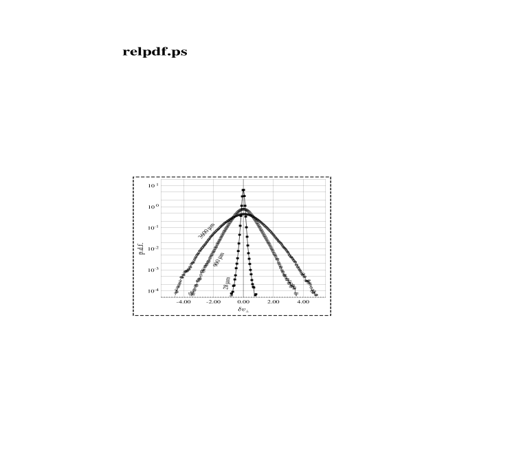
Figure 4: Mesured PDF’s of transverse structure functions [24]

The evaluated probability density functions are compared with the outcome of the measurements of Noullez et. al. [24] on the Figs.2-4. The high quality experimental data on the transverse structure functions were obtained using real-space measurements in the air jet. Thus, for a time being, comparing theory with experiment here we assume that the probability density of the the longitudinal velocity differences has the same shape as the one of transverse velocity differences. The quantitative agreement for $1/4<r/L\leq 1$ is very good. We were not able to plot $P(U,r)$ for very small values of the displacement $r$ but the data on Fig.4 show the tendency of the PDF to the $\delta$-function in the limit $r\rightarrow 0$ in accord with the analytic asymptotics. The Fig.2 presents the same curves, plotted in the coordinates $U/r^{1/3}$. One can see increasing deviations from the gaussian at $r/L=1$ with decrease of the displacement $r$. It is clear from the Figure that the probability density cannot be represented in the scale-invariant form (1). This is the manifestation of the intermittency. The calculation was performed using $Mathematica^{TM}$ which failed to produce the generation function $\phi(k,r)$ with $k>5$. The information on $\phi(k,r)$ with $0<k\leq 5$ was sufficient to calculate $P(U,r)$ with the accuracy $\approx 1-2\%$ in the range of variation $0<U<3-4$ and $1/4<r<1$. The fact that at $r=1$ the PDF must be gaussian serves as a good test of the quality of the numerical procedure.

Using the derived expression for $Z_{2}$, one can easily evaluate correct asymmetric probability density $P(U,r)$ giving the values of the odd-order moments in agreement with experimental data. All one has to do is to introduce a term involving the $sin$-contribution to the Fourier-transform in (26)-(27), generating non-zero odd-order moments. Demanding that $S_{2n+1}(L)=0$ we have from (26):

$$A_{2n+1}\approx-\frac{u_{rms}}{({\cal E}L)^{\frac{1}{3}}}\frac{2n(2n+1)A_{2n}}{(2n+1+B)(\xi_{2n}-\xi_{2n+1}+1)}$$

valid for $n>1$. Setting $u_{rms}\approx({\cal E}L)^{\frac{1}{3}}$ and taking $A_{2}\approx 2$ we obtain:

$$A_{3}\approx-0.8;~{}~{}A_{5}\approx 23.0;~{}~{}A_{7}\approx 650:~{}~{}$$

In the case of the large-scale- driven turbulence the expression for $A_{2n+1}$ is derived in a similar manner:

$$A_{2n+1}=-\gamma A_{2n-2}\frac{2n(2n+1)(2n-1)}{(2n+1+B)(3+\xi_{2n-2}-\xi_{2n+1})}$$

This relation contains two unknowns $\gamma$ and $B$. Assuming universality of the exponents, implying $B=20$, we find from the relation for $A_{3}=-4/5$ that $\gamma\approx 6$. In the correct dimensional units $\gamma\approx 6{\cal E}$. This will be important below for the quantitative comparison of theoretical predictions with experimental data. This result has some interesting consequences. Keeping the amplitudes $A_{2n}$ equal to the ones derived above:

$$A_{5}\approx 14;~{}~{}A_{7}\approx 373;~{}~{}A_{9}\approx 28500;~{}~{}$$

We see that even if the exponents are universal, the amplitudes of the moments are not, meaning that the shape of the probability density can vary from flow to flow. It is interesting that to experimentally observe this effect one has to measure high-order moments since the first few structure functions in different flows, considered here, seem to be close. Hereafter we will be mainly interested in the model (20) which is more closely related to physical experiments.

The expression

$$\phi_{1}(k,r)=\sum_{1}^{\infty}A_{2n+1}r^{\xi_{2n+1}}\frac{(-k)^{2n+1}}{(2n+1)!}$$

is to be substituted into the integral:

$$P_{o}=\frac{1}{\pi}\int_{-\infty}^{\infty}sin(kU)\phi_{1}(k,r)~{}dk$$

to give a total asymmetric PDF $P(U,r)=P_{e}(U,r)+P_{o}(U,r)$. A very accurate parametrization of the central part of the PDF, corresponding to not-too-large values of $U$, illustrating appearence of the asymmetric PDF is:

$$\phi_{1}(k,r)=-\frac{2}{15}rk^{3}\phi(k,r)$$

giving:

$$P(U,r)=P_{e}(U,r)+P_{o}(U,r)=P_{e}(U,r)+\frac{2r}{15}\frac{\partial^{3}P_{e}(U,r)}{\partial U^{3}}$$

This expression is approximate and serves only to illustrate the mechanism of appearence of the experimentally observed asymmetric PDF $P(U,r)$. The central part of the probability density can can be very accurately parametrized by the formula (36) with:

$$P_{e}(U,r)=\frac{N}{r^{\alpha}}e^{-x\tanh\frac{x}{a}}$$

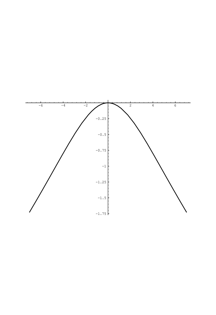
Figure 5: Approximate parametrization of the PDF $r^{\alpha}P(U,r)$ as a vs $x=\frac{U}{r^{\alpha}}$ using formula (37)

where $N$ is a normalization constant, $x\approx\frac{U}{r^{\alpha}}$ with, as above, $\alpha\approx 0.365$. The parameter $a\approx 2~{}-~{}4$. The expression (31)-(32) gives a very good approximation for the moments $S_{n}(r)$ with $n\leq 10$. For example: $A_{2}=1.9-2.6;~{}A_{3}=-0.8;~{}A_{4}=20-28;~{}A_{5}=-15.4-21;~{}A_{6}\approx 657;~{}A_{7}\approx-785;~{}$ etc., very close to the first few amplitudes $A_{n}$, calculated above. Figs. 5-6 show the probability density function $P(U,r)$ given by (36)-(37).

The theory can be approximately generalized to the case of correct anomalous exponents:

$$R_{n}=\frac{S_{n}}{S_{2}^{\frac{n}{2}}}\approx\frac{A_{n}}{A_{2}^{\frac{n}{2}}}r^{\xi_{n}-\frac{n\xi_{2}}{2}}$$

The expression (38) gives $S_{3}$ in accord with the Kolmogorov relation. For $r\approx 0.1$ and $A_{2}\approx 2$ we derive: $R_{3}=-0.31;~{}R_{5}=-4.2;$.

To assess internal consistency of the theory and understand the role and meaning of the $A$-contribution to (20), we write a formally exact equation for the two-point generation function:

$$2\frac{\partial^{2}Z_{2}}{\partial\lambda\partial r}-\frac{2}{\lambda}\frac{\partial Z_{2}}{\partial r}=\lambda^{2}(\kappa(0)-\kappa(|x_{i}-x_{j}|))Z_{2}+I_{T}+I_{p}+D$$

The equation for the probability density $P(U,r)$ can also be formally written:

$$\frac{\partial}{\partial U}U\frac{\partial P}{\partial r}+\frac{\partial P}{\partial r}=-\frac{1}{2}\frac{\partial^{2}}{\partial U^{2}}[T(U,r)P(U,r)]$$

where

$$T(U,r)=<i_{p}+i_{T}+d|~{}U>$$

is the conditional expectation value of $T=i_{p}+i_{T}+d$ for a fixed value of velocity difference $U$. Here $d=d^{\prime}+\nu(u_{x^{\prime}x^{\prime}}(x^{\prime})-u_{xx}(x))$. The formulation of probability density functions in terms of conditional dissipation and production was introduced in [25]-[26] and became a subject of intense investigations. Three-dimensional turbulence problem is somewhat different since there is no way one can separate various contributions to $T(U,r)$. Indeed, we are dealing here with the projection of a three-dimensional dynamics onto a line. This leads to violation of all conservation laws and it is clear that the pressure-induced processes of the correlation- redistribution between different components of velocity, probably conservative in the original equation of motion, can lead to the dissipation-like effects of $T(U,r)$. We can see from the above definitions that due to homogeneity of the turbulence

$$\overline{i_{T}+i_{p}+d}=\int_{-\infty}^{\infty}T(U,r)P(U,r)dU=0$$

It will be shown below that (42) can serve as an equation for determination of the only unknown parameter of the theory $B$. Comparing (40)-(41) with (22) gives:

$$-\frac{1}{2}\frac{\partial}{\partial U}T(U,r)P(U,r)=-\frac{u_{rms}}{L}\frac{\partial}{\partial U}UP(U,r)+(B^{o}-1)\int_{-\infty}^{U}\frac{\partial P(y,r)}{\partial r}dy-A\frac{U}{r}P(U,r)$$

Recalling that $B=-B^{o}>0$ and $A=(3+B)/3>0$, the relations (42)-(43) give an equation for the only unknown coefficient $B>0$. It can be solved numerically to establish consistence with the above calculation leading to $B\approx 20$. An interesting insight into (42)-(43) is obtained if we use the fact that the deviations from scaling of a central part of the PDF are small. This means that:

$$P(U,r)=\frac{1}{r^{\alpha}}F(\frac{U}{r^{\alpha}})$$

Substituting this into (42)-(43) gives:

$$-\frac{1}{2}\frac{\partial}{\partial U}T(U,r)P(U,r)=-\frac{u_{rms}}{L}\frac{\partial}{\partial U}UP(U,r)+\frac{\alpha(B+1)U}{r}P(U,r)-\frac{AU}{r}P(U,r)$$

Now, we have to define the “representative exponent” $\alpha\approx\xi_{n}/n$ with $0<n<3$, which can be done only approximately. Choosing $\alpha=\xi_{1}$ and recalling that $\xi_{1}(B+1)\equiv A$, the last two terms cancel and

$$T(U,r)=2\frac{u_{rms}}{L}U$$

satisfying the constraint (42).

A much more interesting relation is obtained by substituting (36) into (43) with the scale-invariant expression for $P_{e}(U,r)$. Taking into account that $\alpha(B+1)=A$, we have:

$$\frac{T(U,r)}{2}=\frac{2(B+1)(1-3\alpha)}{15P(U,r)}\frac{\partial P_{e}(U,r)}{\partial U}$$

The plot of $T(U,r)$ calculated from (39) using an approximate relation (36)-(37) is presented on Fig. 7 for $r\approx 0.01$. Outside the interval $-2~{}<U/r^{\alpha}<~{}3-4$ the curve saturates which might be an artifact of the exponential asymptotics the approximate formula (36)-(37), valid only when $U$ not too large. It is interesting that the curve is asymmetric, reflecting the asymmetry of the PDF. In the limit $U\rightarrow 0$ the expression (44) gives:

$$T(U,r)\approx\frac{4(B+1)(3\alpha-1)}{15}\frac{U}{r^{2\alpha}}$$

This relation takes into account that $3\alpha>1$. Choosing $\alpha\approx\frac{3+B}{3B}\approx\frac{23}{60}\approx 0.383$ gives:

$$T(U,r)\approx 0.84\frac{U}{r^{2\alpha}}\approx\frac{0.84A_{2}}{r^{0.07}}\frac{U}{S_{2}}$$

where $A_{2}\approx 2$ is the amplitude of $S_{2}(r)$.

Coming back to the estimate of parameter $B$. We saw that setting $\alpha=\xi_{1}$, though shedding some light on the structure of the expression (43), does not allow it’s estimate. The problem is that $S_{1}=0$ and one cannot use it for the non-dimensionalization of the argument of the scale-invariant PDF. A different parametrization $\alpha=\xi_{2}/2$, typically used for analysis of experimental data, leads to cancellation of the last two terms if

$$\frac{\xi_{2}}{2}({B+1})=\frac{B+3}{3}$$

giving $B\approx 40$. With the exponent $\alpha\approx 0.383$, best characterizing the top of the PDF $P_{e}(U,r)$ we have $B\approx 12$. This simple calculation demonstrates consistency of the model for $T(U)$ with the magnitude of the parameter $B\approx 20$, derived above.

The expression (43) can be modified using an identity [27]:

$$i_{1}(U,r)\equiv\frac{\partial P(U,r)}{\partial r}=-\frac{\partial}{\partial U}<\frac{\partial U}{\partial r}|U>P(U,r)\equiv\frac{\partial}{\partial U}I_{1}(U,r)P(U,r)$$

where $I_{1}(U,r)$ is the conditional expectation value of $\frac{\partial U}{\partial r}$ for a fixed value of velocity difference $U$. The equation (43) reads:

$$\frac{\partial}{\partial U}T(U,r)P(U,r)=-\frac{u_{rms}}{L}\frac{\partial}{\partial U}UP(U,r)+(B+1)I_{1}(U,r)P(U,r)-A\frac{U}{r}P(U,r)$$

It is easy to see that

$$\frac{1}{2}\frac{\partial U}{\partial r}=\frac{u(r+\delta)-u(\delta)-u(r)+u(0)}{\delta}=u_{x}(r)-u_{x}(0)$$

This expression shows that experimental and numerical investigations of conditional expectation value of velocity-derivative difference for a fixed value of $U$ is important since the combination

$$[(B+1)<\frac{\partial U}{\partial r}|U>-\frac{B+3}{3}\frac{U}{r}]P(U,r)$$

determines the structure of the probability density. Since $P(U,r)=P(-U,-r)$, we have from (35):

$$T(U,r)=-T(-U,-r)$$

Large-scale corrections to scaling
To complete comparison of the present work predictions with experimental data let us discuss some consequences of the expression (26). Experimental determination of the inertial range is usually done by establishing the interval where the third-order moment $S_{3}(r)\propto r$, in accord with the Kolmogorov relation. As one can see from (26) it is not so easy because of the $O(rS_{2})$ subdominant contribution giving

$$S_{3}\approx-0.8r+O({r^{1.7}})$$

where we set $\xi_{2}\approx 0.7$ and $u_{rms}=L={\cal E}=1$. To make quantitative comparison of this relation with the data we have to restore physical dimensional units. Let us define

$$S_{n}(r)=A_{n}s_{n}\equiv A_{n}({\cal E}r)^{\frac{1}{3}}(\frac{r}{L})^{\xi_{n}-\frac{n}{3}}$$

The relation (26) can be rewritten:

$$\frac{S_{n}}{s_{n}}=A_{n}+\frac{u_{rms}}{({\cal E}L)^{\frac{1}{3}}}\frac{n(n-1)A_{n-1}}{(n+B)(\xi_{n-1}-\xi_{n}+1)}(\frac{r}{L})^{\xi_{n-1}-\xi_{n}+1}$$

The high-Reynolds number experiment [23] was conducted in the atmospheric boundary layer on the tower at $35m$ above the ground. The measured $u_{rms}\approx 1.4m/sec$ and the mean dissipation rate ${\cal E}\approx 0.03\frac{m^{2}}{sec^{3}}$. The measured root-mean-square stream-wise velocity component $u_{rms}$ in the wall-bounded flows is somewhat larger than that of the velocity components perpendicular to the direction of the flow. Since in the relation (26) we are interested in $u_{rms}$, corresponding to the top of the inertial range, a good estimate for $u_{rms}/({\cal E}L)^{\frac{1}{3}}\approx 1$. Taking $L\approx 35m$ and $A_{2}\approx 2.0~{}-~{}2.5$ gives:

$$-\frac{S_{3}}{{\cal E}r}\approx 0.8~{}-~{}(0.06-0.08)r^{0.7}$$

and

$$-\frac{S_{5}}{s_{5}}\approx 20~{}-~{}2r^{0.75}$$

The experimentally observed [23] relation

$$S_{5}=A_{5}({\cal E}r)^{\frac{5}{3}}(\frac{r}{L})^{\xi_{5}-\frac{5}{3}}\approx 0.09r^{1.53}$$

is consistent with numerical values for ${\cal E}$ and $L$ used above. The third and fifth-order moments, calculated from the above relation, are presented on Fig.8. The parameters used were: $A_{5}\approx 20$ and $A_{4}\approx 22$ [23]. The value of the integral scale $L\approx 35m$, used above, can be a bit overestimated. Choosing $L\approx 20-30~{}m~{}$ does not substantially modify the above conclusions. This result is extremely important since it shows that without explicit accounting for the subdominant $O(r^{0.7})$- component of $S_{3}$, one cannot observe the Kolmogorov relation but in very high Reynolds number flows. It also tells us that, in fact, inertial range can be made much broader and the scaling exponents can be established very accurately with the proper data processing. One can see from the Fig.8 that the fifth-order moments starts deviating from its asymptotic value earlier than $S_{3}$. The expressions corresponding to the model (23), can be written easily:

$$\frac{S_{2n+1}}{s_{2n+1}}=A_{2n+1}+\frac{\gamma A_{2n-2}(2n+1)2n(2n-1)}{n+B}(\frac{r}{L})^{3+\xi_{2n-2}-\xi_{2n+1}}$$

As we see, in the limit $r\rightarrow 0$ the contribution from the sub-leading term in this case is much smaller. This means that for a given $Re$ investigation of the scaling exponents $\xi_{n}$ in the numerically- created large-scale-driven turbulence is much easier.

Discussion and Conclusions

The theory developed in this work is based on equations including a simple model for the pressure and dissipation terms. This model, though satisfying all basic symmetry constraints, has not been rigorously derived from the Navier-Stokes equations. The merits of such work can be judged by comparison of theoretical predictions with experimental data. The calculated exponents and the amplitudes of the structure functions $S_{n}(r)$ agree very well with available experimental data. The theory also predicts the large-scale corrections to scaling, thus allowing calculation of $S_{n}$ up to the large-scale cut- off $L$ at which $S_{2n+1}(r)$ become very small. This prediction is non-trivial and can serve as a rigorous test of the model. The scale where it happens is an integral scale of turbulence, corresponding to the top of the inertial range. This definition seems very plausable since it corresponds to the length-scale of the non-zero energy flux set up.

The most straitforward experimental test of this theory can be performed in a following way. Assuming that the odd-order moments have the form:

$$S_{2n+1}=A_{2n+1}r^{\xi_{2n+1}}+B_{2n+1}r^{\beta_{2n+1}}$$

where the exponents $\beta_{n}$, reflecting the large-scale dynamics, have been avaluated above for the two cases of turbulence production. The Log-Log plotting of the functions

$$F_{2n+1}=B_{2n+1}r^{\beta_{n}-\beta_{2n+1}}=-\frac{S_{2n+1}}{r^{\xi_{2n+1}}}-A_{n}$$

will enable one to obtain direct information about the sub-leading contributions to the moments and, as a result, directly assess the quality of the equations for the moments $S_{n}(r)$. The knowledge of $\beta_{n}$ will define universality classes, differing by the mechanisms of turbulence generation. According to this work, the functions $F_{2n+1}$ should demonstrate the scaling behaviour all the way up to the integral scale $L$. If this is indeed so, the measurements are not too difficult.

If turbulence is driven by the large-scale body force, the subleading correction to the Kolmogorov relation for $S_{3}(r)$ is an analytic $O(r^{3})$ function. This flow can be realized in numerical experiments. In the real-life situations this kind of forcing rarely exist. The appearence of the $O(r^{1.7})$ non-analytic correction in the relation for $S_{3}(r)$, derived from the equation (22), can be easily explained in both cases of decaying and sheared turbulence considered above. The measurements in jets and wakes are usually taken at the distance $x$ from the origin (nozzles, bodies etc) where turbulence is produced. Thus, as was stated above, the proper model is that of decaying turbulence at the time $T=x/U$ after turbulence generation at $t=0$, where $U$ is the mean velocity at the crossection $x$. Then, assuming a close-to- self-similar decay the correction is:

$$O(rS_{2t}(r))\approx rS_{2}(r)F_{t}(T)\approx r^{1.7}$$

where the function $F(t)$ describes the time-dependence of $S_{2}(r,t)$ in decaying turbulence. In case of the shear-generated turbulence the correction is [18]:

$$O(r\frac{\partial V}{\partial x}S_{2}(r))\approx r^{1.7}$$

We do not know how general this result is. According to present work, it cannot be universal. The theory makes a direct connection to Landau’s remark about the role of the large-scale fluctuations of turbulence production. We cannot answer the most important question about universality of the exponents: for this we need detailed and quantitative information on the production terms in the equations of motion. However, even if the exponents are universal or belong to some broad universality classes, the probability density function of velocity difference is not universal since the amplitudes of the moments $S_{n}(r)$ depend on some of the features of the non-universal large-scale dynamics and the details of the single-point probability density.

The assumption about gaussian single point PDF, responsible for the values of the amplitudes of the even-order moments, was used here as a good approximation sufficient for demonstration of the basic features of the theory. It is clear that the non-universality of the symmetric part of the PDF $P_{e}(U,r)$ is determined by deviations of the single-point PDF from the gaussian. It is interesting that, according to the present work, even neglecting non-universality of $P_{e}(U,r)$, the asymmetric part $P_{o}(U,r)$, responsible for the odd-order moments, is not universal. This is quite reasonable since the very existence of the flux, reflected in $P_{o}(U,r)$, is the result of the large-scale dynamics.

The theory, presented here, is a departure from all previous field-theoretical attempts to develop an infra-red divergence-free turbulence theory, able to explain anomalous scaling of the moments of velocity difference. It has always been assumed that due to galilean invariance, the vertex corrections are equal to zero in the infra-red limit $k\rightarrow 0$. The supposed GI led to formulation of the Ward identities which were not too helpful. The low- order Kraichnan’s LHDIA [28], which in addition to the conservation laws correctly accounted for such basic symmetries of the problem as random galilean invariance, led to the Kolmogorov energy spectrum without any corrections. It is interesting, that the same approximation, applied to Burgers turbulence, resulted in the $k^{-2}$- energy spectrum corresponding to strong shocks. Kraichnan explained this non-trivial result in terms of the phase-decorrelation due to the interaction between components of the velocity field, non-existent in the Burgers dynamics, which effectively prevents the shock formation. According to [28], it is this decorrelation which is responsible for the formation of the close- to- experimental data Kolmogorov $5/3$-energy spectrum. All attempts to preserve galilean invariance of the theory of three-dimensional turbulence led to disappearence of the integral scale $L$ from the problem and resulting inability of the theory to predict deviations from the Kolmogorov scaling. Polyakov’s [11], Boldyrev [29] and Parisi et. al.[16] theories of Burgers turbulence showed that the galilean invariance is not to be taken for granted: only the low-order moments $S_{n\leq 1}\propto r^{n}$ corresponding to $|U|<<u_{rms}$ can be described in this regime. The structure functions $S_{n}\propto r$ with $n>1$ scale with $u_{rms}$ depending on the large- scale features of the flow. These works stated that galilean invariance is not sacred and departures from it are responsible for the anomalous scaling of the high-order moments observed in Burgers turbulence. The same conclusion was derived in an earlier work [30] predicting

$$\overline{(u(x+r)-u(x)){\cal E}(x){\cal E}(x+r)}\propto u_{rms}(\overline{{\cal E}})^{2}(r/L)^{0}$$

This experimentally confirmed relation [31] explicitly involves the GI breaking $u_{rms}$.

The present work makes an additional step in this direction: it assumes that due to incompressibility, GI in three-dimensional turbulence is broken for all, even small velocity fluctuations. This means that the “normal scaling” does not hold for all moments $n>-1$ which seems to agree with experimental data showing deviations from Kolmogorov scaling of all moments $S_{n}$. Free from the GI restrictions, the vertex corrections are introduced in this paper from the very beginning resulting in the equation of motion for the probability density of velocity difference. This equation is based on some general symmetry properties of the system and satisfies all known realizability constraints.

The theory developed here is based on a few assumptions. First of all, it assumes the existence of a closed equation for longitudinal structure functions $S_{n}(r)$. This is a mere generalization of the Kolmogorov result for a particular case with $n=3$. Physical grounds for the equation for $S_{n}$ are based on the fact the Navier-Stokes non-linearities tend to produce two main effects: the shock-generation due to the advection terms which are balanced by the pressure contributions. An interplay between the two leads to creation of the vortical structures seen in the experimental data. The three-dimensional nature of the structures is lost when one considers projection of the entire dynamics onto a line. All we know is that the shock-production is effectively prevented by the pressure terms leading to invalidation of the bi-fractal description of the pure-Burgers dynamics. We also know that the equation of motions are invariant under transformation $U\rightarrow-U$ and $x\rightarrow-x$ and that the dynamic equation for the $N$-point generation function must satisfy the general fusion rule transforming it, upon point merging, into the equation for the $N-1$-function. These are the physical reasons, responsible for all, but one, contributions to the equation (20).

As was mentioned above, except for the $A$-term in (20), all others are more or less prescribed by the original equation of motion. However, without the $A$-term, the equation (20) contradicts exact relation (42) and thus cannot be correct. I have not been able to find an alternative description, obeying general the fusion rules and symmetries of the problem, and producing solution satisfying (42). For example, one can add the $O(Z_{2})$-contribution to the right side of (19) which does not contradict the basic symmetries. It violates, however, one of the principle constraints of the theory $S_{1}=<U>=0$ and thus, cannot be correct. The success of the Boldyrev theory including this term in description of some of the regimes of Burgers turbulence [28] is based on the fact that, as Polyakov’s work, it describes only the moments $S_{n}$ with $n<1$ and the result $S_{1}=0$ can be achieved using contributions coming from the non-scale invariant terms, which are beyond approximations of Refs.[11].[29]. The same happens in the Parisi et. al theory [16] leading, in accord with the bi-fractal picture, to the PDF consisting of two contributions: responsible for the moments with $n<1$ and $n>1$, respectively. In the present paper we, treating all moments $S_{n}(r)$ with $n>0$ on equal footing, do not have the luxury of satisfying the dynamical constraints using some contributions extraneous to the theory and, as a result, our choice of the allowed terms in the equations of motion is much more narrow. One may also attempt to add

$$h\frac{Z_{2}}{r\lambda}$$

not violating the symmetry of the equation (20). This gives

$$\xi_{n}=\frac{n+h}{n+B}$$

However, since $\xi_{0}=0$, the constant $h=0$.

The equation (22) for the PDF can be rewritten in the limit of small $r$ as:

$$\frac{\partial P}{\partial t}+U\frac{\partial P}{\partial r}+B^{o}\int_{-\infty}^{U}\frac{\partial P(y,r)}{\partial r}dy=\frac{P}{\tau}$$

where $\tau\propto r/U$. The meaning of the $A$- term can be understood from the shape of (48) if we take into consideration that, unlike in the one-dimensional case, the interaction with the transverse components of the velocity field, produces an effective sources and sinks or friction for the longditudinal correlations. Then, (48) is the equation of motion taking these sinks and sources into account in the relaxation- time approximation. In other words $\tau\approx r/U$ is simply the life-time (eddy turn-over time) taking the longditudinal structure to substantially change its shape and size due to interactions with the transverse components. This characteristic time, though plausible, is yet to be derived from the final “microscopic theory”. It is important that the equation (48) is conservative, so that, since $<U>=0$, $S_{0}=1$ . Thus, the right side of (48) describes both sinks and sources. This is consistent with the results of the present paper: in the small-scale limit: $S_{n}\propto r^{\xi_{n}}>>r^{\frac{n}{3}}\approx S_{nB}$ for $n<3$ while $S_{n}<<S_{nB}\propto r$ for all $n>3$. Here $S_{nB}$ is the $n^{th}$-order moment of velocity difference measured in the large-scale-driven Burgers turbulence. This can be seen directly from the equation (48): the PDF tail with $U>0$ grows while the part those with $U<0$ decreases making the Navier-Stokes PDF $P(U,r)$ much more symmetric than the one governing the Burgers dynamics. This means that due to the interaction between different components of the velocity field, the weak structures ($|U|<u_{rms}$), generated by the 3D the Navier-Stokes dynamics are much more intense than their counterparts in the Burgers turbulence. At the same time, due to Kraichnan’s phase decorrelation, the strong structures in the Navier-Stokes turbulence are much weaker than the strong shocks, responsible for the high-order moments of the Burgers dynamics.

In a recent paper by Zikanov et.al. [32] a modified one-dimensional Burgers equation

$$u_{t}+u_{x}u+\alpha u_{x}\int^{\infty}_{-\infty}\frac{u(x^{\prime})}{x-x^{\prime}}~{}dx^{\prime}~{}=~{}f+\nu u_{xx}$$

has been considered. As in Ref. [12], the white-in-time gaussian random force characterized by the spectrum $\overline{|f(k)|^{2}}\propto k^{-1}$ was used. The large scale dissipation was introduced to avoid growth of the mode $u(k=0)$. It has been shown that addition of the non-local contribution is sufficient to prevent the shock formation and generation of the non-trivial exponents $\xi_{n}\neq 1$ for $n>3$. The possible relation of (49) to the equations, introduced in this paper, will be discussed elsewhere.

The good agreement of the scaling exponents of the structure functions wiht experimental data, derived in this paper, though gratifying, is not the most important outcome. The cascade models, not related to the equations of motion, also give quantitatively correct $\xi_{2n}$. However, no model was able to address the problem of the asymmetry of the probability density function $P(U,r)\neq P(-U,r)$ and, as a consequence, predict the scaling exponents and the amplitudes of the odd-order structure functions. Only dynamic theory, based on the Navier-Stokes equations, invariant under transformation $u\rightarrow-u$ and $x\rightarrow-x$ can lead to the asymmetric probability density and correct properties of the odd-order moments.

The present theory, though based on some physical considerations developed for the Burgers equation, is not a small perturbation around Burgers phenomenology: the coefficient $B\approx 20$ and $B>>b\approx 2$ obtained in [11]. Moreover, the relevant coefficient $B^{0}$, renormalizing advection contributions in equation (19), is strongly negative unlike parameter $b>0$ in the theory of Burgers turbulence. This means that the pressure and transverse terms, preventing formation of strong shocks, are extremely important here. On the other hand, the Burgers effects are not unimportant at all. To demonstrate it, we can neglect the “original” Burgers terms in the equation of motion and derive the relation for the moments:

$$S_{n}=A_{n}r^{\kappa_{n}}-\frac{u_{rms}}{L}\frac{A_{n-1}}{A_{n}}n(n-1)\frac{r^{\kappa_{n-1}+1}}{1-\frac{A}{B^{\prime}}}$$

where now

$$\kappa_{n}=\frac{A}{B^{\prime}}n$$

and $A/B^{\prime}<1$. We see that without “small” Burgers terms the equation of motion gives normal scaling and that is why they are essential for derivation of the anomalous scaling exponents. If all this is correct, one may say that the anomalous scaling is the result of the dynamic interplay of the Burgers-like tendency to create singularities (shocks) with the “normalizing” action of the pressure terms and the incompressibility constraints.

The equations developed here are based on the phenomenology relevant for the longitudinal structure functions and that is why we cannot say anything about shape and scaling of transverse structure functions. The main problem is that the odd-order moments $S^{t}_{2n+1}=<(v_{\alpha}({\bf x+r})-v_{\alpha}(\bf x))^{2n+1}>=0$, where vector ${\bf r}$ is parallel and $v_{\alpha}$ is a component of the velocity field perpendicular to the $x$-axis. This means that the PDF $P(\Delta v_{\alpha},r)=P(-\Delta v_{\alpha},r)$ and the equations governing probability density of transverse velocity differences must have different symmetry properties than (20)-(21).

The most important feature of hydrodynamic turbulence, distinguishing it from equilibrium statistical mechanics, is constant energy flux in the wave-number space. It is this energy flux that makes the probability density $P(U,r)$ asymmetric, leading to the non-zero values of the odd-order longitudinal structure functions. It is not clear how the information about the energy flux is reflected in the transverse structure functions coming out from the corresponding symmetric probability density. It is even unclear if $S^{t}_{n}(r)$ are a dynamically relevant object. In the theory presented here, the transverse components of the velocity field simply serve as a “bath” introducing some renormalization and dephasing into the the energy flux- carrying longitudinal dynamics. The angular dependence of the structure functions in three-dimensional turbulence can be recovered using the multidimensional equation for the two-point generating function with the pressure terms accounted for in the mean field approximation, similar to the one introduced in this paper. It is not clear if this can lead to the improved description of experimental data.

Acknowledgments I am grateful to R.H. Kraichnan whose remarks, insights and constructive suggestions were most essential for this work. My thanks are due to S.-Y.Chen, K.R.Sreenivasan, B. Dhruva, R.Miles and U.Frisch for providing me with their most recent, sometimes unpublished, experimental data. Very interesting and stimulating discussions with S. Boldyrev, A. Chekhlov, M. Chertkov, U. Frisch, M. Nelkin, A.Polyakov and B. Shraiman are gratefully acknowledged. This work was supported in part by the ONR/URI grants.

references
1. L.D.Landau and E.M. Lifshitz, Fluid Mechanics, Pergamon Press, Oxford, 1987;   A.S.Monin and A.M.Yaglom, “Statistical Fluid Mechanics” vol. 1, MIT Press, Cambridge, MA (1971)
2. A.N. Kolmogorov, J.Fluid Mech., 5, 497 (1962).    An interesting chain of events starting with Landau’s remark and ending with the Kolmogorov paper is described in: U. Frisch, “Turbulence”, Cambridge University Press, 1995.
3. R.H. Kraichnan, Phys.Rev.Lett.,72, 1016 (1994)
4. F. Gawedzki and A. Kupianen, Phy.Rev.Lett., 75, 3834 (1995)
5. M. Chertkov, G. Falkovich, I. Kolokolov and V.Lebedev, Phys.Rev. E,52, 4924 (1995)
6. M. Chertkov, G. Falkovich, I. Kolokolov and V.Lebedev, Phys.Rev. E,51, 5609 (1995).
7. B. Shraiman and E. Siggia, CR Acad.Sci., 321, Serie II (1995)
8. V.Yakhot, Phys. Rev. E, (1996)
9. M.Vergassola and A.Mazzino, CHAO-DYN/9702014
10. O.Gat, V. L’vov, E. Podivilov and I. Procaccia CHAO-DYN/9610016
11. A.M. Polyakov, Phys.Rev. E 52, 6183 (1995)
12. A. Chekhlov and V. Yakhot, Phys.Rev.E 51, R2739 (1995)
13. A. Chekhlov and V. Yakhot, Phys.Rev. E 52, 5681 (1995)
14. V. Yakhot and A.Chekhlov, Phys.Rev.Lett. 77, 3118 (1996)
15. M. Chertkov, I. Kolokolov and M. Vergassola, preprint
16. J.P. Bouchaud, M. Mezard and G. Parisi, Phys.Rev. E 52 3656 (1995);  V.Gurarie and A.Migdal, Phys. Rev. E54,4908 (1996);  the relation for $S_{4}(r,\theta)$ has been written by M.Nelkin;   A.Chekhlov and V.Yakhot, unpublished (1996)
17. D. Forster, D. Nelson and M. Stephen, Phys. Rev. A16 732 (1977)
18. S. Corrsin, NACA R$\&$M 58B1 (1958); J.L. Lumley, Phys. Fluids 10, 855, (1967); I am grateful to B. Shraiman who brought my attention to these works.
19. S.-Y. Chen, private communication, 1997
20. M. Chertkov, Phys.Rev. E, 55, 2722 (1997)
21. P. Kailasnath, A.A. Migdal, K.R. Sreenivasan, V. Yakhot and L. Zubair, Yale preprint (1991)
22. S.-Y. Chen, private communication, 1997
23. B. Dhruva and K.R. Sreenivasan, private communication (1997)
24. A. Noullez, G. Wallace, W. Lempert, R.B. Miles and U.Frisch, J.Fluid.Mech. 339, 287 (1997)
25. Ya. G. Sinai and V.Yakhot, Phys.Rev.Lett., 63,1962 (1989)
26. S. Pope, Combust. Flame 27, 299 (1976)
27. I am gratefull to R.H.Kraichnan who pointed out this relation to me
28. R. H. Kraichnan, Phys.Fluids. 11, 266 (1968)
29. S. Boldyrev, Phys.Rev.E 55, 6907 (1997)
30. V. Yakhot, Phys.rev. E 50, 20 (1994)
31. A. Praskovskii and S. Oncley, Phys. Rev. E 51, R5197 (1995)
32. O. Zikanov, A. Thess and R. Grauer, Phys.Fluids 9, 1362 (1997)

Figure legends
Fig. 1. Comparison of the calculated scaling exponents (formula (27)) with the results of numerical simulations of Chen [19].
Fig. 2. Probability density of velocity differences $F(x)=r^{\frac{1}{3}}P(\frac{U}{r^{\frac{1}{3}}})$ vs $x=\frac{U}{r^{\frac{1}{3}}}$.
Fig. 3. Probability density $P(U,r)$ as a function of $U/u_{rms}$.
Fig. 4. Mesured PDF’s of transverse structure functions [24] for a few values of the displacement $r=3600\mu m;~{}900\mu m;~{}28\mu m;$.
Fig. 5. Approximate parametrization of the PDF $r^{\alpha}P(U,r)$ vs $x=\frac{U}{r^{\alpha}}$ using formula (37).
Fig. 6. Asymmetric PDF $P(U,r)$ given by (36)-(37).
Fig. 7. Calculated conditional mean $\frac{T(U,r)}{2}$ using approximate expression for the PDF (36)-(37).
Fig. 8. Calculated normalized moments $s_{3}=\frac{S_{3}(r)}{r}$ and $s_{5}=\frac{S_{5}(r)}{r^{1.53}}$.

Figure 1: Comparison of the calculated scaling exponents (formula (27)) with the results of numerical simulations of Chen [19]

Figure 2: Probability density of velocity differences $F(x)=r^{\frac{1}{3}}P(\frac{U}{r^{\frac{1}{3}}})$ vs $x=\frac{U}{r^{\frac{1}{3}}}$

Figure 3: Probability density P(U,r) as a function of U

Figure 6: Asymmetric PDF P(U,r) given by (31)-(32)

Figure 7: Calculated conditional mean $\frac{T(U,r)}{2}$ using approximate expression for the PDF (36)-(37)

Figure 8: Calculated normalized moments $S_{3}(r)$ and $S_{5}(r)$