Cycle expansions for intermittent diffusion

Abstract

We investigate intermittent diffusion using cycle expansions, and show that a truncation based on cycle stability achieves reasonable convergence.

I Introduction

Classical dynamical systems range from purely integrable to purely hyperbolic. For purely integrable systems we have a variety of classical methods, such as separation of the Hamilton-Jacobi equation [1]. For almost integrable systems we have KAM theory [2]. For purely hyperbolic systems it is possible to obtain much information about the system by grouping contributions computed on unstable periodic orbits [3] into terms in cycle expansions [4, 5]. They yield the classical escape rate of open billiard systems to a high degree of accuracy [6], and the semiclassical energy levels of systems such as helium [7] using a surprisingly small number of unstable periodc orbits.

However, the formalism does not work well for generic dynamical flows for which the hyperbolic regions coexist with attractors, intermittent regions and elliptic regions. For intermittent systems the cycle expansions ordered by the topological cycle length converge poorly if very long almost stable cycles dominate the dynamics. The original [4] as well as more recent applications [8] of cycle expansions to intermittent systems use detailed analytic information about the intermittent regions in order to explicitly sum infinite sequences of such cycles.

Our philosophy here is that it should be possible to obtain reliable dynamical averages without a complete understanding of the detailed structure of the phase space, as long as we are restricted to a given connected region in which the dynamics is ergodic. Recent work [9] on the Lorentz gas suggests that reordering the cycle expansions by stability [10] may improve convergence in such situations. Here we test this proposal by calculating diffusion in a one-dimensional intermittent map and demonstrate that the stability ordering yields better convergence than the ordering by the topological cycle length.

There are several arguments in favour of using stability rather than the topological or (in case of continuous flows) real time length as the truncation criterion:

1. Longer but less unstable cycles can give larger contributions to a cycle expansion than short but highly unstable cycles. In such situation truncation by length may require an exponentially large number of very unstable cycles before a significant longer cycle is first included in the expansion.

2. Stability truncation requires only that all cycles up to given stability cutoff be determined, without requiring detailed understanding of the topology of the flow and symbolic dynamics. It is thus much easier to implement for a generic dynamical system than the curvature expansions [4] which rely on finite subshift approximations to a given flow.

3. The stability ordering preserves approximately any shadowing that is present. That is, a long cycle which is shadowed by several shorter ones will have a stability eigenvalue which is approximately the product of the shorter cycle eigenvalues, and will be most likely be included at the same stability cutoff.

4. Cycles can be detected numerically by searching a long trajectory for near recurrences [11, 12]. The method preferentially finds the least unstable cycles, regardless of their topological length. Another practical advantage of the method (in contrast to the Newton method searches) is that it only finds cycles in a given connected ergodic component of phase space, even if isolated cycles or other ergodic regions exist elsewhere in the phase space.

In what follows we illustrate the first three points by investigating the convergence of stability cutoff approach for a simple system. We begin by describing diffusion on a lattice of one-dimensional maps, how to calculate the diffusion coefficient using cycle expansions, and then perform the calculations numerically. Finally we discuss the scope of such approaches and possible improvements.

II Diffusion in 1-D maps

As a model on which to test the above ideas we shall use a well understood one parameter family of diffusive one-dimensional maps. For such maps the symbolic dynamics is a complete binary shift, all cycles can be exhaustively enumerated, and the limitations of the length truncated cycle expansions are solely due to the lack of hyperbolicity, and not to inadequate understanding of the symbolic dynamics.

Many of the features of intermittent systems can be captured by one-dimensional intermittent maps introduced in ref. [13] to study turbulence. Piecewise linear approximations [14] can make statistical mechanics aspects of such intermittent dynamics, including phase transitions [15] and Levy flights, analytically tractable. Intermittent maps can lead to anomalous deterministic diffusion, with the mean square displacement either sublinear or superlinear in the time [16].

In the interval $\hat{x}\in[-1/2,1/2)$, which we call the elementary cell, our model map takes the form

$$\hat{f}(\hat{x})=\hat{x}(1+2|2\hat{x}|^{\alpha})\;\;,$$ (1)

where $\alpha>-1$. For any value of $\alpha$, this maps the interval monotonically to $[-3/2,3/2)$. Outside the elementary cell, the map is defined to have a discrete translational symmetry,

$\displaystyle\hat{f}(\hat{x}+n)=\hat{f}(\hat{x})+n\qquad n\in\cal{Z}\;\;.$

A typical initial $\hat{x}$ in the elementary cell diffuses, wandering over the real line. The map is parity symmetric, $\hat{f}(-\hat{x})=-\hat{f}(\hat{x})\;\;,$ so the average value of $\hat{x}_{n+1}-\hat{x}_{n}$ is zero, and there is no mean drift.

FIG. 1.: The map (1) for $\alpha=1$ restricted to the elementary cell, together with the $0^{6}+$ cycle. In the full space this cycle correspond to ballistic motion to the right, with each 7th iteration entering the next cell.

We now restrict the dynamics to the elementary cell, that is, we define

$\displaystyle x=\hat{x}-[\hat{x}+1/2]\;\;,$

where $[z]$ is the greatest integer less than or equal to $z$, so that $x$ is restricted to the range $[-1/2,1/2)$. The reduced map (see Fig. 1) is

$$f(x)=\hat{f}(x)-[\hat{f}(x)+1/2]\;\;.$$ (2)

A cycle $p=\{x_{1},x_{2},\ldots,x_{n}\},f^{n}(x_{j})=x_{j}$ with stability $\Lambda_{p}=\prod_{j=1}^{n}f^{\prime}(x_{j})$ corresponds to a trajectory which returns to an equivalent point in the full dynamics, $\hat{f}^{n}(x_{j})=x_{j}+\hat{n}_{p}$. Thus the cycles fit into two categories, those which are periodic in the full dynamics, $\hat{n}_{p}=0$, and those which are not. The diffusive properties of the map are fully specified by the reduced map $f(x)$, together with the lattice translation $\hat{n}$. The diffusion constant

$$D=\lim_{n\rightarrow\infty}\frac{1}{2n}\langle\hat{n}^{2}\rangle$$ (3)

is computed as an average over initial conditions in the elementary cell.

The reduced map (2) has three branches, corresponding to either moving to the left, staying in the elementary cell, or moving to the right, $\hat{n}=\{-1,0,1\}$. Hence the natural symbolic dynamics is a 3-letter alphabet $\{-,0,+\}$. For a given symbol string the total translation $\hat{n}$ is just the sum of the individual symbols in the cycle symbol string. The three branches form a Markov partition, because each is mapped onto the whole interval, and the symbolic dynamics is thus unrestricted in the three symbols, with all finite strings corresponding to cycles.

The point $x=0$ is a fixed point (cycle of length 1) with symbol sequence $0$. For $\alpha<0$, $\Lambda_{0}=f^{\prime}(0)=\infty$, this fixed point is infinitely unstable, and its contribution to cycle expansions is vanishing. For $\alpha>0$, $\Lambda_{0}=f^{\prime}(0)=1$, the fixed point is marginally stable and is also customarily omitted from cycle expansions [4]. The intermittent behavior arises from cycles containing long strings of $0$’s which come close to the marginally stable fixed point.

III Cycle expansions

Cycle expansion approaches to deterministic diffusion in one-dimensional maps were introduced in refs. [17, 18] and in the Lorentz gas in ref. [19]. The dynamical zeta function formula [5] for the diffusion coefficient is

$$D=\frac{1}{2}\frac{\sum(-1)^{k}{(\hat{n}_{p_{1}}+\hat{n}_{p_{2}}+\ldots+\hat{n}_{p_{k}})^{2}\over|\Lambda_{p_{1}}\Lambda_{p_{2}}\ldots\Lambda_{p_{k}}|}}{\sum(-1)^{k}{n_{p_{1}}+n_{p_{2}}+\ldots+n_{p_{k}}\over|\Lambda_{p_{1}}\Lambda_{p_{2}}\ldots\Lambda_{p_{k}}|}}\;\;,$$ (4)

where the sum is over nonempty distinct nonrepeating combinations of prime cycles, $\hat{n}$ is the lattice translation of a cycle, $n$ is the period of the cycle, and $\Lambda$ its stability. As the flow is conserved, the leading eigenvalue of the Frobenius-Perron operator equals unity, and the inverse of the corresponding dynamical zeta function [3] must vanish [5] for $z=1$:

$$1/\zeta(1)=1+\sum(-1)^{k}/|\Lambda_{p_{1}}\Lambda_{p_{2}}\ldots\Lambda_{p_{k}}|=0\;\;.$$ (5)

For example, with the $\{-,0,+\}$ symbolic dynamics the cycle expansion up to topological length $n=2$ equals

$\displaystyle 1/\zeta(1)=1-{1\over\Lambda_{+}}-{1\over\Lambda_{-}}-{1\over\Lambda_{+0}}-{1\over\Lambda_{-0}}-{1\over\Lambda_{+-}}+{1\over\Lambda_{+}\Lambda_{-}}\;\;,$

where we have omitted the $0$ cycle.

Ideally the $+-$ cycle is shadowed by the $+$ and $-$ cycles, so the last two terms are expected to approximately cancel. The cancellation is exact when $\alpha=0$ and both terms equal $9$. However, for other values of $\alpha$ shadowing may not lead to any significant cancellations. For example, for $\alpha=1$, $\Lambda_{+}\Lambda_{-}=25$ but $\Lambda_{+-}\approx 12$.

For the case $\alpha=0$ the map $f(x)$ is piecewise linear, $\Lambda=3^{n}$ for all cycles, and in this case the stability and length ordering are equivalent. If the $0$ cycle is included, all $n>1$ terms in (4) cancel, leading to $D=1/3$.

For $\alpha>0$, the dynamics is intermittent, and $\Lambda_{p}$ does not necessarily grow exponentially with cycle length $n_{p}$. Furthermore, for $\alpha>0$ the most stable orbits which contain long strings of $0$’s are not shadowed by combinations of shorter cycles, as the $0$ cycle is not included. In fact, we can explicitly deduce the behavior of the most stable cycles, those of the form $0^{n}+$ (an example is given in Fig. 1). These begin at initial point which we shall denote by $x_{n}$, slightly greater than zero. Many iterations of the function increase monotonically the value of $f^{k}(x)$ until it finally crosses over to the right branch and returns to the starting point. Inserting an extra $0$ in the symbolic dynamics has the effect of slightly decreasing the starting point, but the other cycle values are virtually unchanged, the new starting point is very close to the old one, and $f(x_{n+1})=x_{n}$ is a good approximation for moderately large $n$. Thus for $\alpha>0$

$\displaystyle\frac{x_{n}}{x_{n+1}}\approx 1+2(2x_{n+1})^{\alpha}$

to the leading order in $x_{n}$. This difference equation may be approximately solved as a power law, $x_{n}=\gamma n^{-\delta}$ giving $\alpha\delta=1$, $2(2\gamma)^{\alpha}=\delta$, or

$\displaystyle x_{n}=\frac{1}{2(2\alpha n)^{1/\alpha}}\;\;.$

The stability can be estimated in a similar fashion:

$\displaystyle\frac{\Lambda_{n}}{\Lambda_{n-1}}\approx f^{\prime}(x_{n})=1+2(\alpha+1)(2x_{n})^{\alpha}=1+\frac{\alpha+1}{\alpha n}\;\;.$

Again putting $\Lambda_{n}=\rho n^{\epsilon}$ we obtain $\epsilon=1+1/\alpha$,

$\displaystyle\Lambda_{n}\sim n^{1+1/\alpha}\;\;,$

confirmed by our numerical results. This power-law growth of $\Lambda_{n}$ is in contrast to hyperbolic systems for which all cycles have stabilities which grow exponentially with the cycle length.

Because these are the most stable cycles, they dominate cycle expansions at given $n$. Combinations of cycles which do not include a cycle with a string of almost $n$ $0$’s are highly suppressed. For example, two cycles with $n/2$ $0$’s and one other symbol each have a combined stability

$\displaystyle\Lambda_{n/2}^{2}\sim(n^{2}/4)^{1+1/\alpha}\gg\Lambda_{n}$

for large $n$, again in contrast with hyperbolic systems, for which such shadowing combinations are of comparable magnitude. Hence we can estimate the convergence properties of such cycle expansions by approximating them with the dominant $0^{n}+$ cycle family [4]. In this approximation the flow conservation condition (5)

$$1/\zeta(1)\sim\sum_{n}{1\over n^{1+1/\alpha}}\;\;,$$ (6)

is approximately the Riemann zeta function $\zeta(1+1/\alpha)$, convergent for all $\alpha>0$, which is just as well. The denominator in the diffusion formula (4) appears whenever we calculate the time average of some quantity, and plays the role of a mean cycle period

$$\langle n\rangle_{\zeta}\sim\sum_{n}{1\over n^{1/\alpha}}\;\;.$$ (7)

As $\alpha$ increases, the system spends more and more of its time near the marginally stable fixed point, and for $\alpha\geq 1$, the system spends on average all of its time within an arbitrarily small neighborhood of this point, leading to a divergent mean cycle period (7). The numerator of the expression for diffusion looks like the flow conservation sum (6), with extra factors of $\hat{n}_{p}^{2}$. This factor is a number of order unity for the least unstable cycles, so the series converges. Thus the average (4) which defines the diffusion coefficient undergoes a phase transition [15] and equals zero for $\alpha\geq 1$. This behavior is described as “weak” ($0<\alpha<1$) or “strong” ($\alpha\geq 1$) intermittency. Other averages may converge for different ranges of $\alpha$.

For $\alpha\geq 1$ the diffusion is anomalous, with $\langle\hat{n}^{2}\rangle$ increasing more slowly than $n$. In the case at hand

$\displaystyle 1/\zeta(z)\sim\sum_{n}{z^{n}\over n^{1+1/\alpha}}\sim\left\{\begin{array}[]{ll}(z-1)&\alpha<1\\ (z-1)\ln(z-1)&\alpha=1\\ (z-1)^{1/\alpha}&\alpha>1\end{array}\right.\;\;,$

and the leading behavior of a dynamical zeta function as $z\rightarrow 1$ yields [18] the exponent characterizing the sublinear diffusion

$\displaystyle\langle x_{n}^{2}\rangle\sim\left\{\begin{array}[]{ll}n&\alpha<1\\ n/\ln n&\alpha=1\\ n^{1/\alpha}&\alpha>1\end{array}\right.\;\;.$

We are now in position to estimate and compare the rates of convergence of the topological and stability truncation approaches. As we have seen, the cycle expansions are dominated by terms of the form $1/n^{\gamma}$ where $\gamma=1+1/\alpha$ for the flow conservation condition, and $\gamma=1/\alpha$ for the diffusion constant. Thus the error made by the topological truncation length after $n$ terms is $\sim n^{1-\gamma}$. In contrast, truncating by stability corresponds to an error of order of $\Lambda^{-1/(\alpha+1)}$ for the flow conservation, and $\Lambda^{(\alpha-1)/(\alpha+1)}$ for the diffusion constant. For $\alpha\to 1$ close to where the expansion diverges it may be advisable to improve the estimates by convergence acceleration techniques.

Having defined the cycle expansions and analyzed their behavior in the intermittent case, we now pose the more pragmatic question: What is the optimal ordering in practice? In the approximation we have been using, with only a single family of cycles contributing, the ordering is self-evident. However, the full expansion is only conditionally convergent, and as we have no proof that the stability ordering yields the correct results, our justification will come from heuristic arguments, together with the numerical results.

The topological length cutoff corresponds to a complete partitioning of the phase space into $3^{n}$ periodic point neighborhoods, irrespective of the relative sizes of these neighborhoods. What is the meaning of the stability cutoff? A cycle expansion can be interpreted [5] as a partition of the dynamical phase space into neighborhoods of periodic points $i\in p$, each of size $\sim 1/\Lambda_{p}$. A fixed stability cutoff $\Lambda$ selects a uniform partition of the phase space into $\sim\Lambda$ regions, each of period approximately $N=\ln\Lambda$, the time needed for a neighborhood of a hyperbolic orbit to spread across the entire system. Each prime cycle has about $N$ periodic points, so the number of prime cycles up to a given stability grows as $\Lambda/\ln\Lambda$. This estimate is known as the dynamics version of the prime number theorem for Axiom A systems, given in ref. [20]. We find that the estimate is valid numerically for nonhyperbolic systems as well, in the case at hand for all values of $\alpha>-1$.

The dramatic difference between the two approaches is the number of cycles required in each case. The number of prime cycles up to a given length increases exponentially with the length, in our case as $\sim 3^{n}/n$. The number of prime cycles up to a given stability is grows as $\Lambda/\ln\Lambda$. Superficially, the topological ordering requires an exponential number of cycles, while the stability ordering requires only a power law. The issue is how small is the error for a given truncation. In the case of nice hyperbolic flows this error is superexponentially small, but for intermittent systems, the size of the error is not known, and we have to resort to numerics to estimate it.

IV Numerical results

For a simple one-dimensional map with a complete symbolic dynamics, such as the map (1) studied here, almost any reasonable cycle finding method [5] should yield thousands of prime cycles. The accuracy of $1/\Lambda$’s that we calculate approaches the machine precision. We implement the stability ordering by noting that for this map any cycle containing an extra symbol is less stable than the preceding one. We recursively increment cycle lengths, starting with $+$ and $-$, and stopping when the stability cutoff is reached. The stability ordering is fast, as cycles containing large numbers of $0$’s which dominate the expansion appear only a few times in this enumeration. The distribution of cycles as a function of $n_{p}$ and $\Lambda_{p}$ is shown in Fig. 2.

FIG. 2.: The distribution of cycle eigenvalues as a function of the topological cycle length: For $\alpha=1$, the intermittent case, a fixed topological length $n$ cutoff misses many of the least unstable (but longer period) cycles.

In Fig. 3 we present a comparison of how well different truncations respect the flow conservation rule (5). There is a definite improvement as the stability cutoff is increased, demonstrating convergence. For smaller values of $\alpha$ there is a significant amount of scatter due to a small number of unbalanced shadowing terms which vary rapidly with $\alpha$, however the error is consistently small. For example, for $\alpha<1$ the error curve corresponding to $\Lambda=10^{5}$ cutoff always lies below $e^{-6}\approx 0.0025$ .

FIG. 3.: Numerical test of the flow conservation for different truncations. The logarithm of the magnitude of the zeta function (5) is plotted as a function of $\alpha$ for stability cutoffs $\Lambda=$ $10^{2}$, $10^{3}$, $10^{4}$, and $10^{5}$ (plusses, open triangles, squares and circles, respectively), as well as for the topological length cutoff $N=10$ (filled circles). The solid curves for $\alpha>0.5$ are the behavior expected from the previous section, $\ln\left(1.5\Lambda^{-\alpha-1}\right)$, for the cutoff values of $\Lambda$, with the constant $1.5$ chosen to fit the data.

The filled circles in Fig. 3 are obtained by using all cycles with $N\leq 10$, corresponding to roughly the same computational effort as the stability cutoff of $10^{5}$. The error is smooth but large, comparable to the stability cutoff only at $\alpha=0$, the solvable case.

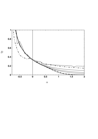
FIG. 4.: Diffusion constant (3) as function of $\alpha$ computed by 3 different methods. The dotted line is obtained by direct numerical evaluation of (3) for $3\times 10^{4}$ random initial points, each evolved by $3\times 10^{4}$ iterations of the map. The dot-dash line is the cycle expansion average (4) truncated at topological length $N=10$, corresponding to $9381$ cycles with $0$ omitted. The expansion is accurate only near $\alpha=0$, where the shadowing is exact. The solid lines are cycle expansions (4) truncated according to stability, with cutoff $\Lambda=10^{2}$ for the uppermost line at $\alpha=2$, followed by $10^{3}$, $10^{4}$ and $10^{5}$ for the other curves. The dashed line is an extrapolation (8) of these curves. $\alpha=1$ corresponds to a phase transition point beyond which $D=0$; all numerical methods fail here.

The diffusion constant, evaluated using three different methods, is plotted as a function of $\alpha$ in Fig. 4. Each of the three methods used about half an hour of computing time for each value of $\alpha$. There is no analytic expression for $D$ in general, except for $D=1/3$ at $\alpha=0$ and $D=0$ for $\alpha\geq 1$, as explained above.

The cycle expansions (4) truncated at topological length $N=10$ (dot-dash line) give very poor estimates of $D$ as $\alpha$ increases away from zero into the intermittent regime, as many of the least unstable cycles are not included (Fig. 2). More surprisingly, even for $\alpha<0$, the hyperbolic phase dominated by exponentially many unstable cycles, the estimate is poor, this time in the opposite direction, because there are many omitted cycles near the $+$ and $-$ cycles with large displacements and moderate stability, $\Lambda\sim\Lambda_{+}^{n}$. The stability of the $+$ and $-$ cycles is $\Lambda_{+}=3+2\alpha$ which is relatively small in this case.

The cycle expansions (4) truncated according to stability (solid lines) approach the direct simulation (dotted line) as the cutoff is increased from $10^{2}$ (upper curve at $\alpha=2$) to $10^{5}$. Since the number of prime cycles less than $\Lambda$ is asymptotically equal to $\Lambda/\ln\Lambda$, we expect that about $10^{5}/\ln 10^{5}\approx 8700$ cycles would be needed, not far from the number of cycles actually found, which lies in the range $8871$-$10066$ for all the $\alpha$ shown.

Due to the phase transition all three methods are only logarithmically convergent to zero at $\alpha=1$. Direct simulation cannot yield accurate estimates of $D$ near this point; the stability and topological length truncations could easily be improved by using the analytic structure of the $0^{n}+$ series [8] for the map at hand, but as we are unlikely to have this information available in a generic case, such improvements are outside the scope of the present investigation.

As discussed in the previous section, we expect that the error should scale as a power of the cutoff stability, related to $\alpha$, or exponentially with $n$ for a cutoff of $10^{n}$. If the convergence of a sequence is exponential and reasonably smooth, it should be possible to extrapolate to the limit using a variety of convergence acceleration schemes. We have tried Aitken’s $\delta^{2}$-process [21]. If $t_{n-1}$, $t_{n}$ and $t_{n+1}$ are three consecutive terms of a sequence, an improved estimate is

$$t_{n}^{{}^{\prime}}=t_{n+1}-\frac{(t_{n+1}-t_{n})^{2}}{t_{n+1}-2t_{n}+t_{n-1}}\;\;.$$ (8)

Using this formula for the cycle expansions computed to a stability of $10^{3}$, $10^{4}$ and $10^{5}$ we obtain the dashed line in Fig. 4, which is comparable to the direct simulation, and much closer to the true value of $D$ than the value obtained by the length cutoff.

It should be noted that the estimate (8) only works if the sequence is relatively smooth. Cycle expansions with stability cutoff are not particularly smooth as a function of the cutoff, for example see Fig. 5 of ref. [9]. This is because at each stage a small number of shadowing combinations are unbalanced by the cutoff, and the number of such mismatches varies rapidly with the cutoff. In this case, the convergence over the range $10^{3}$-$10^{5}$ is sufficiently smooth to use (8), however a smaller spacing such as $2.5\times 10^{4}$, $5\times 10^{4}$, $10^{5}$ is dominated by fluctuations.

V Conclusion

Our results indicate that cycle expansions may be used to calculate averages for intermittent systems with accuracy comparable to direct simulations, as long as a stability cutoff is used. Stability ordering has a great simplicity in that it requires no knowledge of the dynamics, except what is contained in a finite cycle set. We conclude with a few possibilities for future directions.

First, it is good to see rapidly converging expansions, but another thing to have rigorous limits to guarantee convergence. Chaotic systems often behave more nicely than it is possible to prove, however it would be advantageous to extend the proofs of superexponential convergence for length ordered cycle expansions of analytic hyperbolic systems to the stability ordered case, hopefully allowing a wider class of dynamical systems.

The stability ordering exhibits imperfect shadowing, which can lead to scatter in the results, as observed in Fig. 3. One possible remedy to this problem might be to replace the factor $1/\prod\Lambda$ by $f(\prod\Lambda)/\prod\Lambda$ where the smoothing function $f$ moves continuously from $1$ to $0$. This must certainly improve the shadowing, but it requires that cycles be found up to the largest stability at which $f$ is non-zero, without utilizing these cycles fully. For our diffusion coefficient calculations, the results are smooth enough to use Aitken’s method, so additional smoothing is probably unnecessary.

We also note, that because the number of cycles less than a given $\Lambda$ is roughly $\Lambda/\ln\Lambda$, independent of the dimension of the space, stability ordering should be applicable to high dimensional systems. In particular, the detailed structure of the dynamics need not be known, only an algorithm for finding the cycles in the first place, for example tracing out a long trajectory and looking for near repeats, which are then refined by some form of Newton’s method.

Finally, it is not clear to what extent the stability cutoff approach is applicable to quantum systems. It is not as easy to estimate the rate of convergence in this case, even for nice hyperbolic flows, because the terms are complex, and the alternation of the Maslov phase within families of cycles analogous to the $0^{n}+$ family studied above crucial for quantum convergence can lead to large errors in the stability cutoff cycle expansion truncations [22].

REFERENCES

- [1] H. Goldstein, Classical Mechanics (Addison-Wesley, Reading, 1980); V.I. Arnold, Mathematical Methods in Classical Mechanics (Springer-Verlag, 1978, Berlin).
- [2] G. C. Benettin, L. Galgani, A. Giorgilli and J. M. Strelcyn, Nuovo Cimento B 79, 201 (1984).
- [3] D. Ruelle, Statistical Mechanics, Thermodynamic Formalism, (Addison-Wesley, Reading MA, 1978).
- [4] R. Artuso, E. Aurell, and P. Cvitanović, Nonlinearity 3, 325 (1990); 3, 361 (1990).
- [5] P. Cvitanović, et al, Classical and Quantum Chaos: A Cyclist Treatise, http://www.nbi.dk/ChaosBook/, Niels Bohr Institute (Copenhagen 1997)
- [6] P. Cvitanović and B. Eckhardt, Phys. Rev. Lett. 63, 823 (1989); P. Gaspard and D. Alonso Ramirez, Phys. Rev. A 45, 8383 (1992); P. Cvitanović, P.E. Rosenqvist, H.H. Rugh, and G. Vattay, CHAOS 3, 619 (1993).
- [7] D. Wintgen, K. Richter, and G. Tanner, CHAOS 2, 19 (1992).
- [8] P. Dahlqvist, Nonlinearity 8, 11 (1995); 10, 159 (1997); J. Stat. Phys. 84,773 (1996). J. Phys. A 30, L351 (1997). G. Tanner and D. Wintgen, Phys. Rev. Lett. 75, 2928 (1995).
- [9] C. P. Dettmann and G. P. Morriss, Phys. Rev. Lett. 78, 4201 (1997).
- [10] P. Dahlqvist and G. Russberg, J. Phys. A 24, 4763 (1991).
- [11] D. Auerbach, P. Cvitanović, J.-P. Eckmann, G.H. Gunaratne and I. Procaccia, Phys. Rev. Lett. 58, 2387 (1987).
- [12] G. P. Morriss and L. Rondoni, J. Stat. Phys. 75, 553 (1994).
- [13] Y. Pomeau and P. Manneville, Commun. Math. Phys. 74, 189 (1980).
- [14] P. Gaspard and X.-J. Wang, Proc. Natl. Acad. Sci. USA 85, 4591 (1988); Phys. Rev. A 40, 6647 (1989).
- [15] P. Cvitanović, in P. Zweifel, G. Gallavotti and M. Anile, eds., Non-linear Evolution and Chaotic Phenomena (Plenum, New York 1987); R. Artuso, P. Cvitanović and B.G. Kenny, Phys. Rev. A 39, 268 (1989).
- [16] T. Geisel and S. Thomae, Phys. Rev. Lett. 52, 1936 (1984); T. Geisel, J. Nierwetberg, and A. Zachel, Phys. Rev. Lett. 54, 616 (1985).
- [17] R. Artuso, Phys. Lett. A 160, 528 (1991).
- [18] R. Artuso, G. Casati, and R. Lombardi, Phys. Rev. Lett. 71, 62 (1993).
- [19] W. N. Vance, Phys. Rev. Lett. 69, 1356 (1992); P. Cvitanović, J.-P. Eckmann and P. Gaspard, Chaos, Solitons and Fractals 6, 113 (1995); P. Cvitanović, P. Gaspard, and T. Schreiber, CHAOS 2, 85 (1992).
- [20] W. Parry and M. Pollicott, Ann. Math. 118, 573 (1983).
- [21] W. H. Press, S. A. Teukolsky, W. T. Vetterling, and B. P. Flannery, Numerical Recipes in C, Second Ed., 166 (Cambridge University, Cambridge, 1992).
- [22] S.F. Nielsen, Univ. of Copenhagen Master’s thesis (1997), available on http://www.nbi.dk/ChaosBook/ .