Cycling chaos: its creation, persistence and loss of stability in a model of nonlinear magnetoconvection

Abstract

We examine a model system where attractors may consist of a heteroclinic cycle between chaotic sets; this ‘cycling chaos’ manifests itself as trajectories that spend increasingly long periods lingering near chaotic invariant sets interspersed with short transitions between neighbourhoods of these sets. This behaviour can be robust (i.e., structurally stable) for systems with symmetries and provides robust examples of non-ergodic attractors in such systems; we examine bifurcations of this state.

We discuss a scenario where an attracting cycling chaotic state is created at a blowout bifurcation of a chaotic attractor in an invariant subspace. This is a novel scenario for the blowout bifurcation and causes us to introduce the idea of set supercriticality to recognise such bifurcations. The robust cycling chaotic state can be followed to a point where it loses stability at a resonance bifurcation and creates a series of large period attractors.

The model we consider is a $9$th order truncated ordinary differential equation (ODE) model of three-dimensional incompressible convection in a plane layer of conducting fluid subjected to a vertical magnetic field and a vertical temperature gradient. Symmetries of the model lead to the existence of invariant subspaces for the dynamics; in particular there are invariant subspaces that correspond to regimes of two-dimensional flows. Stable two-dimensional chaotic flow can go unstable to three-dimensional flow via the cross-roll instability. We show how the bifurcations mentioned above can be located by examination of various transverse Liapunov exponents. We also consider a reduction of the ODE to a map and demonstrate that the same behaviour can be found in the corresponding map. This allows us to describe and predict a number of observed transitions in these models.

and

1 Introduction

There has been a lot of recent interest in the chaotic dynamics of nonlinear systems that possess invariant subspaces; a number of quite subtle dynamical effects come to light in examining the interaction of attractors with the invariant subspaces. Moreover a good understanding of these effects is essential in interpreting and predicting dynamics of simulations and experiments where the presence of discrete spatial symmetries implies the existence of invariant subspaces.

A fundamental bifurcation in such a setting is the blowout bifurcation [16] where a chaotic attractor within an invariant subspace loses stability to perturbations transverse to the invariant subspace. In doing so, can either create a nearby ‘branch’ of chaotic attractors or lose stability altogether.

In contrast with this, the presence of invariant subspaces can lead to the existence of what have been called robust heteroclinic cycles [11] between equilibria, that is, heteroclinic cycles that are persistent under small perturbations that preserve the symmetry. These cycles may or may not be attracting [13]. Recently it has been recognised that cycles to more complicated invariant sets can also occur robustly in symmetric systems, in particular to chaotic invariant sets; this behaviour was named ‘cycling chaos’ in a recent paper by Dellnitz et al. [9] and has been further investigated by Field [10] and Ashwin [2].

In this paper we find there is a connection between these dynamical properties; we show a scenario where a blowout bifurcation creates an attracting ‘cycling chaotic’ state in a bifurcation that is analogous to a saddle-node homoclinic bifurcation with equilibria replaced by chaotic invariant sets. We also investigate how the attracting cycling chaotic state that is created in the blowout bifurcation loses stability at a resonance of Liapunov exponents. (A resonance bifurcation in its simplest form occurs when a homoclinic cycle to an equilibrium loses attractiveness; this occurs when the real parts of eigenvalues of the linearisation become equal in magnitude [7].) In spite of the system being neither a skew product nor being a homoclinic cycle to a chaotic set as in [2] we see similar behaviour and can predict the loss of stability by looking at a rational combination of Liapunov exponents.

We find this scenario of a blowout bifurcation to cycling chaos is a mechanism for transition from stable two-dimensional to fully three-dimensional magnetoconvection. The model we study is a Galerkin truncation for magnetoconvection in a region with square plan, subject to periodic boundary conditions on vertical boundaries and idealised boundary conditions on horizontal boundaries. Phenomenologically speaking we see a change from a chaotically varying two-dimensional flow (with trivial dependence on the third coordinate, and which comes arbitrarily close to a trivial conduction state) to an attracting state where trajectories spend increasingly long times near one of two symmetrically related two-dimensional flows interspersed with short transients. We explain and investigate this transition in terms of a blowout bifurcation of a chaotic attractor in an invariant subspace.

In the paper of Ott and Sommerer [16] that coined the phrase ‘blowout bifurcation’, two scenarios are identified. Either the blowout was supercritical in which case it leads to an on-off intermittent state [17], or it is subcritical and there is no nearby attractor after the bifurcation. We find an additional robust possibility for bifurcation at blowout.

Near this transition the three-dimensional flow patterns show characteristics of intermittent cycling between two symmetrically related ‘laminar’ states corresponding to two-dimensional flows, but the time spent near the laminar state is, on average, infinite. This suggests that the blowout is supercritical, but in a weaker sense which we make precise. Namely, we say a blowout is set supercritical if there is a branch of chaotic attractors after the blowout whose limit contains the attractor in the invariant subspaces before the blowout. In particular there may be other invariant sets contained in this limit and so any natural measures on the bifurcating branch of attractors (if they exist) need not limit to the natural measure of the system on the invariant subspace.

We also show that the attractors corresponding to two-dimensional flows are not Liapunov stable, but are Milnor attractors near the transition to three dimensions, and so in particular we expect the presence of noise to destabilise two-dimensional attractors near blowout by a bubbling type of mechanism [4].

We find in our example that the state of cycling chaos is attracting once it has been created: trajectories cycle between neighbourhoods of the chaotic sets within the invariant subspaces, and the time between switches from one neighbourhood to the next increases geometrically as trajectories get closer and closer to the invariant subspaces. By estimating the rate of increase of switching times, we are able to show that cycling chaos ceases to be attracting in a resonance bifurcation. One remarkable aspect of this study is that we are able to predict the parameter values at which the blowout bifurcation and the resonance occur, requiring only a single numerical average over the chaotic set within the invariant subspace.

The paper is organised as follows: in section 2 we introduce the ODE model for magnetoconvection, discuss its symmetries and corresponding invariant subspaces. This is followed by a description of the creation, persistence and loss of stability of the cycling chaos on varying a parameter in numerical simulations in Section 3. Section 4 shows how one can, under certain assumptions, derive a map model of the dynamics of the ODE that has the same dynamical behaviour. Section 5 is a theoretical analysis of the blowout bifurcation that creates the cycling chaotic attractor and is followed in Section 6 by a theoretical analysis of its loss of stability. Finally, Section 7 discusses some of the implications of this work on the chaotic dynamics of symmetric systems.

2 An ODE model for magnetoconvection

The model we study is an ODE on $\mbox{\bf R}^{9}$ described by the following equations

$$\dot{x}_{0} = \mu x_{0}+x_{0}\theta-x_{2}x_{1}-\beta y_{0}^{2}x_{0},$$

$$\dot{x}_{1} = -\nu x_{1}+x_{0}x_{2},$$

$$\dot{x}_{2} = -\sigma x_{2}-\sigma Qa+\gamma x_{0}x_{1},$$

$$\dot{y}_{0} = \mu y_{0}+y_{0}\theta-y_{2}y_{1}-\beta x_{0}^{2}y_{0},$$

$$\dot{y}_{1} = -\nu y_{1}+y_{0}y_{2},$$ (1)

$$\dot{y}_{2} = -\sigma y_{2}-\sigma Qb+\gamma y_{0}y_{1},$$

$$\dot{a} = \zeta(x_{2}-a),$$

$$\dot{b} = \zeta(y_{2}-b),$$

$$\dot{\theta} = -\theta-x_{0}^{2}-y_{0}^{2}.$$

These ODEs have been derived as an asymptotic limit of a model of three-dimensional incompressible convection in a plane layer, with an imposed vertical magnetic field; for further details and details of its derivation, see [14, 19, 20]. In the context of this model, $x_{0}$ and $y_{0}$ represent the amplitudes of convective rolls with their axes aligned in the $y$ and $x$ (horizontal) directions respectively, $x_{1}$ and $y_{1}$ represent modes that cause the rolls to tilt, and $x_{2}$ and $y_{2}$ represent shear across the layer in the $x$ and $y$ directions. The modes $a$ and $b$ represent the horizontal component of the magnetic field in the $x$ and $y$ directions, and $\theta$ represents the horizontally averaged temperature.

The model has are five primary parameters: $\mu$ is proportional to the imposed temperature difference across the layer, with $\mu=0$ at the initial bifurcation to convection; $\beta$ is related to the horizontal spatial periodicity length, but is an arbitrary small parameter in the model of [14, 19]; $\sigma$ and $\zeta$ are dimensionless viscous and magnetic diffusion coefficients; and $Q$ is proportional to the square of the imposed magnetic field. Note that $\sigma$, $\zeta$ and $Q$ are scaled by factors of $4$, $4$ and $\pi^{2}$ from their usage in [14, 19, 20]. Two secondary parameters that we use are $\gamma=3(1+4\sigma)/16\sigma$ and $\nu=(9\sigma/(1+4\sigma))-\mu$. In the parameter regime of interest, all parameters are non-negative.

2.1 Symmetries of the model

Consider $\mbox{\bf D}_{4}\dot{+}T^{2}$ acting on the plane with unit cell $[0,2\pi)^{2}$ in the usual way, with the torus $T^{2}$ acting by translations on the plane, and $\mbox{\bf D}_{4}$ by reflections in the axes and rotation through $\pi/2$. We define the following group elements

$$\kappa_{x}\colon{}$$ reflection through ,

reflection through ,

reflection through ,

reflection through ,

rotation about ,

translation .

(2)

Note that $\rho$, $\tau_{(\xi,\eta)}$ and any reflection $\kappa$ can be used to generate the group $\mbox{\bf D}_{4}\dot{+}T^{2}$.

Table 1: Selected fixed point subspaces $S$ of the action of $G$ on $\mbox{\bf R}^{9}$ together with name, representative point and dimension of $S$. There are others (e.g. $(0,x,0,0,0,0,0,0,t)$) but these are not important for the dynamics we discuss here.

$S$	Name	Representative point	$\dim S$
$F$	Full symmetry	$(0,0,0,0,0,0,0,0,t)$	1
$R_{x}$	$x$-rolls	$(x,0,0,0,0,0,0,0,t)$	2
$R_{y}$	$y$-rolls	$(0,0,0,x,0,0,0,0,t)$	2
$D_{+}$	$+$ diagonal	$(x,0,0,x,0,0,0,0,t)$	2
$D_{-}$	$-$ diagonal	$(x,0,0,-x,0,0,0,0,t)$	2
$R_{xy}$	Mixed modes	$(x,0,0,y,0,0,0,0,t)$	3
$P_{x}$	$x$-rolls + shear	$(x,y,z,0,0,0,a,0,t)$	5
$P_{y}$	$y$-rolls + shear	$(0,0,0,x,y,z,0,a,t)$	5
$Q_{x}$	$x$-rolls + shear + crossrolls	$(x,y,z,w,0,0,a,0,t)$	6
$Q_{y}$	$y$-rolls + shear + crossrolls	$(w,0,0,x,y,z,0,a,t)$	6
$T$	No symmetry	$(u,v,w,x,y,z,a,b,t)$	9

Figure 1: A portion of the isotropy lattice for the action of $G$ on $\mbox{\bf R}^{9}$ under which (2) is equivariant. We have shown fixed point subspaces of some conjugate subgroups separately for clarity. The isotropies of $P_{x}$ and $P_{y}$ are the smallest isotropies that physically involve only two-dimensional effects.

We consider the subgroup

$$G=\langle\kappa_{x},\kappa_{x}^{\prime},\kappa_{y},\kappa_{y}^{\prime},\rho\rangle.$$ (3)

Since $G$ contains the subgroup $(\mbox{\bf Z}_{2})^{2}$, generated by $\kappa_{x}\kappa_{x}^{\prime}$ and $\kappa_{y}\kappa_{y}^{\prime}$, of translations $T^{2}$, it follows that $G$ is isomorphic to a semidirect product $\mbox{\bf D}_{4}\dot{+}(\mbox{\bf Z}_{2})^{2}$ ($|G|=32$). The ODE (2) is equivariant under the group $G$ of symmetries acting on $\mbox{\bf R}^{9}$ by

$$\kappa_{x}(x_{0},x_{1},x_{2},y_{0},y_{1},y_{2},a,b,\theta)= (x_{0},-x_{1},-x_{2},y_{0},y_{1},y_{2},-a,b,\theta),$$

$$\kappa_{x}^{\prime}(x_{0},x_{1},x_{2},y_{0},y_{1},y_{2},a,b,\theta)= (-x_{0},x_{1},-x_{2},y_{0},y_{1},y_{2},-a,b,\theta),$$ (4)

$$\rho(x_{0},x_{1},x_{2},y_{0},y_{1},y_{2},a,b,\theta)= (y_{0},-y_{1},-y_{2},x_{0},x_{1},x_{2},-b,a,\theta).$$

This action gives rise to a number of isotropy types, shown in Table 1. Figure 1 gives a partial isotropy lattice for this group action. Dynamics in $F$ always decays to the trivial equilibrium point, corresponding to the absence of convection. We refer to dynamics in $P_{x}$ and $P_{y}$ as two-dimensional, since these correspond to two-dimensional convection in the original problem (though $\dim P_{x}$ is 5). Dynamics in $R_{x}$ and $R_{y}$ corresponds to mirror symmetric two-dimensional rolls with their axes aligned along the $y$ and $x$ directions; we refer to equilibrium points in these subspaces as $x$-rolls and $y$-rolls respectively. In $P_{x}$ and $P_{y}$, convection is two-dimensional but not mirror symmetric, and is referred to as tilted rolls. Dynamics in $Q_{x}$ and $Q_{y}$ corresponds to three-dimensional convection that is still invariant under one mirror reflection (tilted rolls with a cross-roll component). Otherwise we say the dynamics is fully three dimensional.

In a slight break from convention we say the fixed point subspaces $S$ as having isotropy subgroup $\mathop{\mathrm{Iso}}(S)$ rather than considering the isotropy subgroups as the fundamental objects.

3 Numerical simulations of the ODEs

We present numerical simulations of the ODEs that demonstrate two aspects of cycling chaos that we seek to explain: how cycling chaos can be created in a blowout bifurcation, and how cycling chaos can cease to be attracting.

We concentrate on parameter values that are known to have Lorenz-like chaotic dynamics within $P_{x}$ and $P_{y}$:

$$\mu=0.1655,~{}~{}Q=1/\pi^{2},~{}~{}\sigma=0.125~{}\mbox{ and }~{}\zeta=0.05$$ (5)

(and hence $\nu=0.5845$ and $\gamma=2.25$), although we note that qualitatively similar attractors are found for a large proportion of nearby parameter values. These parameter values correspond to those in Figures 15(c) and 20(a) in [20]. The numerical method used was a Bulirsch–Stoer adaptive integrator [18], with a tolerance for the relative error set to $10^{-12}$ for each step.

We use the parameter $\beta$ as a normal parameter (see [5]) for the dynamics in $P_{x}$ and $P_{y}$; that is, it controls instabilities transverse to $P_{x}$ and $P_{y}$ in the directions $Q_{x}$ and $Q_{y}$ without altering the dynamics inside $P_{x}$ or $P_{y}$.

3.1 Cycling chaos

Figure 2: Numerical solutions of the model ODEs with $\mu=0.1655$, $Q=1/\pi^{2}$, $\sigma=0.125$, $\zeta=0.05$ and $\beta=2.0$. (a) $x_{0}$ against time; (b) $y_{0}$ against time; (c) $x_{0}$ against $x_{2}$; (d) $x_{0}$, $y_{0}$ and $|x_{2}|+|y_{2}|$ in perspective. The crosses in (c) and (d) represent the $x$-roll, $y$-roll and trivial equilibrium points in $R_{x}$, $R_{y}$ and $F$. Note that the chaotic attractor is close to a heteroclinic cycle that connects the $x$-rolls, the $y$-rolls and the trivial fixed point.

In Figure 2 we show a typical example of timeseries when there is attracting cycling chaos (with $\beta=2.0$). The system starts with $x_{0}$ oscillating chaotically while $y_{0}$ is quiescent, switches to a state where $y_{0}$ oscillates chaotically while $x_{0}$ is quiescent, and so on. A more careful examination reveals that after a switch the trajectory remains close to a fixed point in $R_{x}$ or $R_{y}$ for an increasing length of time. Physically, this corresponds to chaotic two-dimensional convection that switches between rolls aligned in the $x$ and $y$ directions. Figure 2(c) shows the chaotic trajectories projected onto the $(x_{0},x_{2})$ plane, while (d) illustrates switching between $P_{x}$ (the ‘horizontal’ plane) and $P_{y}$ (the ‘vertical’ plane).

Figure 3: Numerical solutions of the model ODEs: cycling chaos with (a) $\beta=2.00$, (b) $\beta=1.80$, (c) $\beta=1.65$ and (d) $\beta=1.63$, showing the values of $|x_{0}|$ at which the trajectory intersects the surface defined by $|x_{2}|+|y_{2}|=0.01$. The rising exponential growth phases correspond to the system switching from chaos in $P_{y}$ to chaos in $P_{x}$. The time between switches increases as the system approaches the attracting cycling chaos, but the rate of increase depends on $\beta$.

Note how the chaotic behaviour in Figure 2(a) and (b) repeats: trajectories spend longer and longer near the unstable manifolds of the $x$-roll and $y$-roll equilibrium points and take longer and longer between each switch. This is illustrated further in Figure 3, which shows intersections of a trajectory with the Poincaré surface $|x_{2}|+|y_{2}|=0.01$ close to the trivial solution. There are two phases evident in the cycle: the order one chaotic behaviour of $x_{0}$ near $P_{x}$ (while $y_{0}$ grows exponentially), and the exponential growth of $|x_{0}|$ as the trajectory moves away from $P_{y}$ (while $y_{0}$ behaves chaotically). The time between switches increases monotonically and the rate of increase varies with $\beta$, the normal parameter. In these numerical simulations, the switching time saturates when certain components of the solution come close to the machine accuracy of the computations (about $10^{-323}$ for double precision).

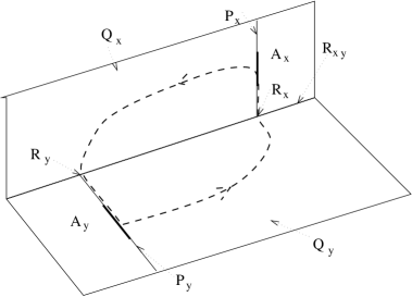
Figure 4: A schematic illustration of the location of the robust cycle relative to the invariant subspaces forced by symmetry. The cycle is between the chaotic invariant sets $A_{x}$ and $A_{y}$ (within $P_{x}$ and $P_{y}$) and two fixed points contained in $R_{x}$ and $R_{y}$. The cycle is robust to $G$-equivariant perturbations that fix the dynamics in $P_{x}$ and $P_{y}$. The intersection of $P_{x}$ and $P_{y}$ at the trivial solution is not shown, although $A_{x}$ and $A_{y}$ do in fact intersect there.

We argue that this is evidence for attracting cycling chaos: trajectories approach a structurally stable heteroclinic cycle between chaotic sets. In Figure 4 we show a schematic picture of the heteroclinic cycle. We recall that the fixed point spaces $R_{x}$ and $R_{y}$ are 2 dimensional, $R_{xy}$ is 3 dimensional, $P_{x}$ and $P_{y}$ are 5 dimensional and $Q_{x}$ and $Q_{y}$ are 6 dimensional invariant subspaces in the 9 dimensional phase space. The system starts near the $x$-roll equilibrium point in $R_{x}$, which is unstable to shear ($x_{2}$); the parameters are such that the unstable manifold of $x$-rolls comes close to the trivial solution and returns to a neighbourhood of $x$-rolls. This global near-connection within $P_{x}$ is the source of the chaotic behaviour. We refer to the chaotic sets in $P_{x}$ and $P_{y}$ as $A_{x}$ and $A_{y}$ respectively; these contain the relevant roll equilibrium points and they both contain the trivial solution, so there are structurally stable connections from the trivial solution to the roll equilibrium points and from those to $A_{x}$ and $A_{y}$. Within $Q_{x}$, $A_{x}$ is unstable to cross-rolls ($y_{0}$) since the trivial solution is equally unstable in the $x_{0}$ and $y_{0}$ directions. Eventually $y_{0}$ grows large enough that there is a switch to the $y$-roll equilibrium point in $R_{y}$, at which point $y_{2}$ starts to grow. Thus the cycle connects invariant sets in the following fixed point subspaces:

$$\dots\rightarrow R_{x}\rightarrow P_{x}\rightarrow Q_{x}\rightarrow R_{y}\rightarrow P_{y}\rightarrow Q_{y}\rightarrow\dots$$ (6)

between the equilibrium points in $R_{x}$ and $R_{y}$, and $A_{x}$ and $A_{y}$ within $P_{x}$ and $P_{y}$, with the structurally stable connections needed to complete the cycle from $A_{x}$ and $A_{y}$ to the $y$-roll and $x$-roll equilibrium points lying within $Q_{x}$ and $Q_{y}$.

Note that our scenario is certainly a simplification of the full set of heteroclinic connections; there are other fixed points contained in the closure of the smallest attracting invariant set, in particular the origin is contained within the cycle.

3.2 Blowout

Figure 5: Numerical solutions of the model ODEs. The top panel (a) shows the chaotic time dependence of $x_{0}$, independent of $\beta$, and the lower three panels show the blowout bifurcation: (b) $\beta=3.50$, before the blowout bifurcation (solutions decay to two-dimensional chaos); (c) $\beta=3.47$ near the blowout bifurcation; and (d) $\beta=3.40$ after the blowout bifurcation (solutions grow to cycling chaos). The straight lines show the average growth or decay rates predicted by the Liapunov exponents calculated using (27).

We turn now to the question of how the cycling chaos is created. With $\beta=3.5$ we find attracting two-dimensional chaos (Figure 5a, b), which loses stability around $\beta=3.47$ (c) in a blowout bifurcation, and for $\beta=3.40$ (d), there is exponential growth away from $P_{x}$ into $Q_{x}$. Within $Q_{x}$, the $y$-roll equilibrium points are sinks, establishing the structurally stable connection from the chaos in $P_{x}$ to the equilibrium point in $R_{y}$, and hence the creation of cycling chaos.

3.3 Resonance

Figure 6: Time intervals between switches between $P_{x}$ and $P_{y}$ with $\beta$ in the range $1.60$–$1.64$. The intervals between switches increase by a factor of about $1.03$ and $1.02$ per switch for $\beta=1.64$ and $1.63$ respectively. The switching times stop increasing once the values of variables become so small that the cubic terms in the ODEs cannot be represented accurately with double-precision numbers (and calculations were terminated once any variable went below $10^{-100}$). For $\beta=1.61$ and $1.60$, the system approaches a periodic orbit and the intervals between switches goes to a constant (though in the case of $\beta=1.61$, the periodic orbit is only achieved after 1500 switches).

As illustrated in Figures 3, as $\beta$ decreases towards $1.63$, trajectories spend progressively longer in each visit to $P_{x}$ and $P_{y}$ before switching to the conjugate chaotic invariant set. Eventually, trajectories come arbitrarily close to the invariant subspaces $P_{x}$ and $P_{y}$ (limited only by machine accuracy in the numerical simulations). Figure 6 shows how the time intervals between switches between $A_{x}$ and $A_{y}$ increases as the system approaches this heteroclinic cycle, and how the rate of approach to the heteroclinic cycle decreases as $\beta$ approaches $1.62$. The intervals between switches grow by a factor of about $1.4$, $1.2$ and $1.1$ per switch for $\beta=2.00$, $\beta=1.80$ and $\beta=1.65$ respectively, and $1.03$ and $1.02$ for $\beta=1.64$ and $1.63$. By $\beta\approx 1.62$, the heteroclinic cycle is no longer attracting, and for $\beta=1.61$ and $1.60$, the system settles down to periodic behaviour that is bounded away from $P_{x}$ and $P_{y}$, though the periodic orbits are actually quite close to these invariant subspaces. For these calculations, we imposed a cut-off of $10^{-100}$: the calculation ceased once any variable became smaller than this.

In the next section, we derive a map that allows us to compute longer trajectories more accurately, and we demonstrate cycling chaos, its creation in a blowout bifurcation and its loss of attractiveness using this map. We analyse the blowout bifurcation in section 5, and argue in section 6 that the cycling chaos created in that bifurcation ceases to be attractive at a resonance.

4 Reduction to a map

In this section, we discuss a map that models the behaviour of the ODEs in the parameter regime described above, and that helps clarify what happens near blowout bifurcation and the resonance of the cycling chaos.

4.1 Derivation

We rely on a map derived for the two-dimensional dynamics by breaking up the flow into pieces near and between equilibrium points [20]. Within the $P_{x}$ subspace, the leading stable eigendirection of the origin (that is, the eigendirection with negative eigenvalue closest to zero) is in the $(x_{2},a)$ plane, and the unstable direction of the origin is along the $x_{0}$ axis. All trajectories leaving the origin in that direction follow the structurally stable connection within $R_{x}$ to one or other of the $x$-roll equilibrium points. The one-dimensional unstable manifold of $x$-rolls lies within $P_{x}$, and the chaotic attractor is associated with a global bifurcation at which that unstable manifold collides with the origin. Near this global bifurcation, the dynamics within $P_{x}$ is modelled by an augmented Lorenz map:

$$(x_{0},x_{2}=\pm 1)\mapsto\left(\mathop{\mathrm{sgn}}(x_{0})(-\kappa+C_{1}|x_{0}|^{\delta_{1}}),-x_{2}\right)$$ (7)

defined as a map from the surface of section $|x_{2}|=h$ to itself. Details of the derivation are given in [20], but briefly, $\kappa$ is a parameter related to $\mu$ in the ODEs, with $\kappa=0$ at the global bifurcation; $h$ is a small positive constant that we scale to one; $\mathop{\mathrm{sgn}}(x)=+1$ if $x>0$ and $-1$ if $x<0$; $\delta_{1}$ depends on the ratio of various stable and unstable eigenvalues at the origin and the $x$-roll equilibrium points (with $0<\delta_{1}<1$); and $C_{1}$ is a (negative) constant.

It is a straightforward matter to include the effect of a small perturbation in the $y_{0}$ and $y_{2}$ directions. Near the $P_{x}$ subspace, $y_{0}$ and $y_{2}$ will grow linearly at a rate that depends on $x_{0}$. This means that we get a mapping of the form

$$(x_{0},x_{2}=\pm 1,y_{0},y_{2})\mapsto{}$$ (8)

$$\left(\mathop{\mathrm{sgn}}(x_{0})(-\kappa+C_{1}|x_{0}|^{\delta_{1}}),-x_{2},C_{2}y_{0}|x_{0}|^{\delta_{2}},C_{3}y_{2}|x_{0}|^{\delta_{3}}\right),$$

where $C_{2}$ and $C_{3}$ are constants and the exponents $\delta_{2}$ and $\delta_{3}$ again depend on ratios of eigenvalues, with $\delta_{2}<0$ and $\delta_{3}>0$. The exponent $\delta_{2}$ is negative since a small value of $x_{0}$ implies that the trajectory spends longer near the origin, so $y_{0}$ has a longer time to grow. Similarly, near $P_{y}$ we get the mapping

$$(x_{0},x_{2},y_{0},y_{2}=\pm 1)\mapsto{}$$ (9)

$$\left(C_{2}x_{0}|y_{0}|^{\delta_{2}},C_{3}x_{2}|y_{0}|^{\delta_{3}},\mathop{\mathrm{sgn}}(y_{0})(-\kappa+C_{1}|y_{0}|^{\delta_{1}}),-y_{2}\right),$$

as long as $x_{0}$ is much smaller than $y_{0}$.

These maps are valid provided that the trajectory remains close to the $P_{x}$ or $P_{y}$ subspaces. We model the switch from behaviour near $P_{x}$ to near $P_{y}$ by assuming that (8) holds provided that $|x_{0}|>|y_{0}|$; otherwise, the trajectory leaves the neighbourhood of the origin along the $y_{0}$-axis, visits a $y$-roll equilibrium point and returns to the surface of section $|y_{2}|=1$ near the origin:

$$(x_{0},x_{2}=\pm 1,y_{0},y_{2}) \mapsto \left(C_{4}x_{0}|y_{2}|^{\delta_{4}}|y_{0}|^{\delta_{2}},\pm C_{5}|y_{2}|^{\delta_{5}}|y_{0}|^{\delta_{3}},\right.$$

$$\phantom{\left(\right.\kern-2.4pt}\left.\mathop{\mathrm{sgn}}(y_{0})(-\kappa+C_{6}|y_{2}|^{\delta_{6}}|y_{0}|^{\delta_{1}}),\mathop{\mathrm{sgn}}(y_{2})\right),$$

where, as above, $C_{4}$, $C_{5}$ and $C_{6}$ are constants and $\delta_{4}$, $\delta_{5}$ and $\delta_{6}$ are ratios of eigenvalues. Similarly, (9) holds if $|x_{0}|<|y_{0}|$; otherwise the trajectory switches from $P_{y}$ to $P_{x}$:

$$(x_{0},x_{2},y_{0},y_{2}=\pm 1) \mapsto{} \left(\mathop{\mathrm{sgn}}(x_{0})(-\kappa+C_{6}|x_{2}|^{\delta_{6}}|x_{0}|^{\delta_{1}}),\mathop{\mathrm{sgn}}(x_{2}),\right.$$

$$\phantom{\left(\right.\kern-2.4pt}\left.C_{4}y_{0}|x_{2}|^{\delta_{4}}|x_{0}|^{\delta_{2}},\pm C_{5}|x_{2}|^{\delta_{5}}|x_{0}|^{\delta_{3}}\right).$$

Then in the full map, as long as $|x_{0}|>|y_{0}|$, the trajectory behaves chaotically under (8) (near the $P_{x}$ subspace), with $x_{0}$ obeying a Lorenz map and $y_{0}$ growing or decaying according to the value of $x_{0}$. If $y_{0}$ grows sufficiently that $|y_{0}|>|x_{0}|$, there is one iterate of map (4.1), which makes $x_{0}$ small as the system switches from $P_{x}$ to $P_{y}$, followed by many iterates of (9), and one iterate of (4.1) as the system switches back to $P_{x}$.

The $\delta$ exponents can be determined from the eigenvalues of the trivial solution and of $x$-rolls. The relevant eigenvalues of the origin are (in the notation of [20]) the growth rate $\mu$ of $x_{0}$ and $y_{0}$ and the slowest decay rate $\lambda_{\zeta}$ of $(x_{2},a)$, determined by the eigenvalue of

$$\left[\matrix{-\sigma&-\sigma Q\cr\zeta&-\zeta\cr}\right]$$ (12)

closest to zero. The relevant eigenvalues of $x$-rolls are the growth rate $\lambda^{+}$ and the slowest decay rate $\lambda_{2}^{-}$ of $(x_{1},x_{2},a)$, determined by the eigenvalues of

$$\left[\matrix{-\nu&\sqrt{\mu}&0\cr\gamma\sqrt{\mu}&-\sigma&-\sigma Q\cr 0&\zeta&-\zeta\cr}\right].$$ (13)

The other important eigenvalues at the $x$-roll equilibrium point are the decay rate of $y_{0}$ ($-\beta\mu$) and the decay rate of $y_{2}$ ($\lambda_{\zeta}$). Then we have

$$\delta_{1} = \frac{\displaystyle-\lambda_{\zeta}}{\displaystyle\mu}\left(1+\delta_{6}\right),\qquad\delta_{2}=\frac{\displaystyle-\lambda_{\zeta}}{\displaystyle\mu}\delta_{4}-1,\qquad\delta_{3}=\frac{\displaystyle-\lambda_{\zeta}}{\displaystyle\mu}\left(1+\delta_{5}\right),$$

$$\delta_{4} = \frac{\displaystyle\beta\mu}{\displaystyle\lambda^{+}},\qquad\delta_{5}=\frac{\displaystyle-\lambda_{\zeta}}{\displaystyle\lambda^{+}},\qquad\delta_{6}=\frac{\displaystyle-\lambda_{2}^{-}}{\displaystyle\lambda^{+}}.$$ (14)

From fitting the map to trajectories of the ODEs with $\beta=3.47$ (see Figure 5b), we find values for the constants:

$$\kappa = -0.014072,$$

$$C_{1}=-0.12450,\qquad C_{2} = 0.27200,\qquad C_{3}=0.16791,$$ (15)

$$C_{4}=609.65,\qquad C_{5} = 0.86515,\qquad C_{6}=0.0015974.$$

The eigenvalues that do not depend on $\beta$ are:

$$\lambda_{\zeta}=-0.059697,\qquad\lambda^{+}=0.29606,\qquad\lambda_{2}^{-}=-0.048978.$$ (16)

With these eigenvalues, we have $\delta_{1}=0.42038$, $\delta_{3}=0.43344$, $\delta_{5}=0.20164$ and $\delta_{6}=0.16543$, while $\delta_{2}$ (negative) and $\delta_{4}$ depend on $\beta$.

4.2 Iterating the map

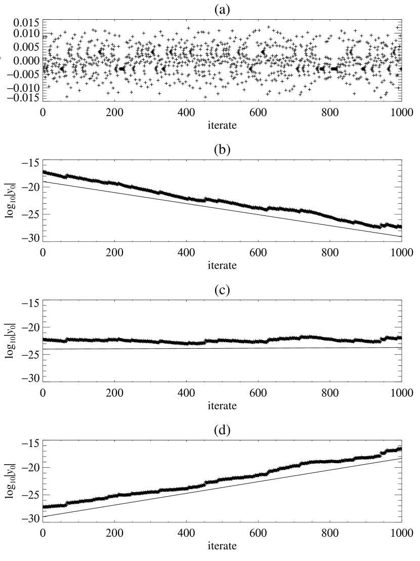
Figure 7: Blowout in the map (8–4.1): compare with Figure 5. (a) Chaotic behaviour of $x_{0}$ near $P_{x}$. For different values of $\beta$ (b: $\beta=3.89$, c: $\beta=3.87$, d: $\beta=3.85$), the distance from $P_{x}$ as measured by $|y_{0}|$ decays in (b) and grows in (d). The blowout bifurcation occurs for parameters near (c). The straight lines show the average growth or decay as predicted by (29), averaged over 1000 iterates.

We seek to reproduce in the map what we have observed in the ODEs: the blowout bifurcation that creates cycling chaos, and the loss of attractiveness of cycling chaos. The first of these (Figure 7) is straightforward: typical Lorenz-like chaos is shown in Figure 7(a), while the change from decay towards $P_{x}$ to growth away from $P_{x}$ at $\beta\approx 3.87$ is shown in (b–d).

Figure 8: Resonance in the map (8–4.1): compare with Figures 3 and 6. (a) and (b): $\beta=1.100$, showing the approach to cycling chaos and the increase in number of iterates between switches ($\rho=1.011$). (c) and (d): $\beta=1.088$, showing growth away from cycling chaos ($\rho=0.9984$) and saturation to a periodic orbit. The dashed lines in (c) and (d) show the predicted rate of increase or decrease of the switching times from (39).

Cycling chaos is found after the blowout bifurcation (Figure 8a): the system switches between chaos in $P_{x}$ and chaos in $P_{y}$, getting closer and closer to the invariant subspaces after each switch and spending longer between switches (Figure 8b). The rate of increase of the intervals between switches depends on $\beta$, and is about a factor of 1.01 per switch for $\beta=1.10$. Decreasing $\beta$ to $1.088$ (Figure 8c,d) results in growth away from cycling chaos and saturation to a periodic orbit.

These calculations required formulating the map (8–4.1) in terms of the logarithms of the variables in order to cope with the large ($10^{1000}$) dynamic range. The one place in which accuracy is inevitably lost is in the switch from $P_{x}$ to $P_{y}$ (and back), using (4.1): the $C_{6}|y_{2}|^{\delta_{6}}|y_{0}|^{\delta_{1}}$ term is swamped by the order one $\kappa$. As a result of this, the chaotic trajectories start in exactly the same way each time the system switches from one invariant subspace to the other.

In terms of the ODEs, the trajectory entering a neighbourhood of $P_{x}$ close to $x$-rolls shadows the unstable manifold of that equilibrium point (lying inside $P_{x}$ and leading to the chaotic set $A_{x}$) until the switch to $P_{y}$. This is in agreement with the ODE behaviour shown in Figure 2.

5 Analysis of the blowout bifurcation

We briefly review some definitions. If $A$ is a compact flow-invariant subset then we define the unstable set

$${\cal W}^{u}(A)=\{x\in\mbox{\bf R}^{9}~{}:~{}\alpha(x)\subseteq A\}$$ (17)

and the stable set (or basin of attraction)

$${\cal W}^{s}(A)=\{x\in\mbox{\bf R}^{9}~{}:~{}\omega(x)\subseteq A\}$$ (18)

where $\alpha(x)$ (resp. $\omega(x)$) is the limit set of a trajectory of the ODE passing through $x$ in the limit $t\rightarrow-\infty$ (resp. $\infty$). We say a compact invariant set $A$ is an attractor in the sense of Milnor if

$$\ell({\cal W}^{s}(A))>0$$ (19)

where $\ell(\cdot)$ is Lebesgue measure on $\mbox{\bf R}^{9}$. It is said to be a minimal Milnor attractor if there are no proper compact invariant subsets $S\subset A$ with $\ell({\cal W}^{s}(A)\setminus{\cal W}^{s}(S))>0$ [15].

As shown in [1], Milnor attractors can occur in a robust manner if the attractor lies within an invariant subspace. Suppose $P$ is an invariant subspace and $A$ is a compact invariant set in $P$ such that $A$ is a minimal Milnor attractor for the flow restricted to $P$ and such that $A$ has a natural ergodic invariant measure $\mu$ for the flow restricted to $P$. It is possible to show (under certain additional hypotheses [1]) that $A$ as an attractor in the full system if and only if $\Lambda(\mu)<0$, where $\Lambda$ is the most positive Liapunov exponent for $\mu$ in a direction transverse to $P$ (see [5] for a detailed discussion). If we have access to a normal parameter [5] such that we can vary the normal dynamics without changing the dynamics in $P$, we can vary $\Lambda$ through zero and observe loss of attractiveness of $A$ at what Ott and Sommerer have termed a blowout bifurcation [16].

5.1 Set criticality of a blowout bifurcation

Ott and Sommerer identify two possible scenarios at blowout. At a supercritical blowout the attractor bifurcates to a family of attractors displaying on-off intermittency [17], with trajectories that come arbitrarily close to $A$ and thus linger near $A$ for long times (but with a well-defined mean length of lingering or ‘laminar phase’). At subcritical blowout there are no nearby attractors after loss of stability of $A$. Note that [3] discusses the question of how to distinguish these cases.

However, what we see in this paper is that there is at least one other possibility at blowout bifurcation that is also robust to normal perturbations, namely a bifurcation to a cycling state or a robust heteroclinic cycle between chaotic invariant sets. This can be seen to be set supercritical but not supercritical, in the following sense.

By reparametrising if necessary we can assume that we have a normal parameter

$$c=\Lambda(\mu)$$ (20)

so $A$ undergoes a blowout bifurcation at $c=0$. By the argument above, $A$ is an attractor only if $c<0$.

If there is a family of minimal Milnor attractors $A_{c}$, $c>0$ such that for all $\epsilon>0$

$$\overline{\bigcup_{c\in(0,\epsilon)}A_{c}}\supseteq A$$ (21)

then we say that the blowout is set supercritical. Note that as discussed in [16] and implied by the very word ‘blowout’, we cannot typically expect the limit of the attractors to just be the set $A$.

If in addition $A_{c}$ supports a family of natural ergodic invariant measures $\mu_{c}$ ($c>0$) and $\mu_{c}\rightarrow\mu$ as $c\rightarrow 0$ then we say the blowout is measure supercritical or just supercritical. (Convergence is the in the $C^{*}$ topology on probability measures.) This definition of criticality was used in [3].

If the blowout is not set supercritical then we say the blowout is subcritical.

It seems that one will often get bifurcations in symmetric systems that are set supercritical but not supercritical. For example one can generically get a blowout from a group orbit of attractors (under a finite group) which yields a single attractor that limits onto the whole group orbit. Moreover, in the cycling chaos studied here, the attractor after blowout includes not only the chaotic invariant sets, but also fixed points involved in the heteroclinic cycle. As it is a cycle, it does not possess a natural ergodic invariant measure [21] and averages of observables from the system in this state will typically not converge but continue to oscillate more and more slowly.

The blowout scenario described above holds only for variation of normal parameters; in general the variation of a parameter will affect both the normal dynamics and the dynamics within the invariant subspace. If the dynamics in the invariant subspace is chaotic, we can expect to see a large number of bifurcations happening within the invariant subspace and these will cause the blowout to be spread over an interval of parameter values; there is no reason why $\Lambda(\mu_{x})$ should vary continuously with a parameter that varies $\mu_{x}$ in a very discontinuous manner.

Nevertheless, for the numerical results presented in Section 3 the dynamics in the invariant subspace vary in quite regular way. This is because in our system the parameter $\beta$ is a normal parameter for the attractor $A_{x}$; for more discussion of normal parameters, see [5, 8].

5.2 Evidence of blowout bifurcation in the ODE model

By mechanisms described in [20] the pure $x$ and $y$ chaotic dynamics corresponding to dynamics within $P_{x}$ and $P_{y}$ respectively can become chaotic by means of a symmetric global bifurcation that generates Lorenz-like attractors approaching the equilibrium solution with full symmetry and $x$-roll or $y$-roll equilibrium solutions in $R_{x}$ or $R_{y}$.

Now suppose there exist chaotic attractors $A_{x}$ and $A_{y}$ contained in $P_{x}$ and $P_{y}$ (on average they have more symmetry), From here on we will mostly discuss $A_{x}$ but note that as $A_{y}$ is a conjugate attractor, the same will hold for $A_{y}$.

These attractors contain a saddle equilibrium $e$ in $F$ (the trivial solution) and so in particular they cannot be Liapunov stable attractors. This is because $W^{u}(e)\cap P_{x}$ must be non-trivial manifold (otherwise $e$ is an attractor; thus $W^{u}\cap P_{y}$ is also non-trivial as $\mathop{\mathrm{Iso}}(P_{y})$ is conjugate to $\mathop{\mathrm{Iso}}(P_{x})$. Therefore

$${\cal W}^{u}(A_{x})\not\subseteq A_{x}$$ (22)

and so $A_{x}$ cannot be Liapunov stable. However it is possible that $A_{x}$ is an attractor in the sense of Milnor; this will imply that the basin will be locally riddled in the sense of [5].

We assume that $A_{x}$ and $A_{y}$ are minimal Milnor attractors containing $e$. We also assume that they have natural ergodic invariant measures $\mu_{x}$ and $\mu_{y}$ supported on them. We now concentrate on $A_{x}$. Whether $A_{x}$ is an attractor depends on its the spectrum of normal Liapunov exponents. Note that the zero Liapunov exponent corresponding to time translation always corresponds to a perturbation tangential to the invariant subspace. If

$$\Lambda(\mu_{x})<0,$$ (23)

where $\Lambda(\mu)$ is the most positive normal Liapunov exponent for the measure $\mu$, it is possible to show that $A_{x}$ satisfies (19) [5], and hence that $A_{x}$ is a Milnor attractor.

It is comparatively easy to compute $\Lambda(\mu_{x})$ in that case, as the largest transverse Liapunov exponent of $A_{x}$ in the parameter regime discussed corresponds to directions in the $Q_{x}$ direction, where linearised perturbations are described by

$$\dot{y}_{0}=\left(\mu+\theta(t)-\beta x_{0}(t)^{2}\right)y_{0}.$$ (24)

Thus we can see that

$$\Lambda(\mu_{x})=\mu+\langle\theta\rangle_{\mu_{x}}-\beta\langle x_{0}^{2}\rangle_{\mu_{x}},$$ (25)

where $\langle f(x)\rangle_{\mu}=\int f(x)d\mu(x)$. From the equation for $\dot{\theta}$ it is possible to show that

$$\lim_{T\rightarrow\infty}\frac{1}{T}\int^{T}\theta\,dt=\lim_{T\rightarrow\infty}\frac{1}{T}\int^{T}x_{0}^{2}\,dt$$ (26)

along bounded trajectories of the ODE. For the given parameter values it is possible to approximate $\langle\theta\rangle_{\mu_{x}}=-0.03703$ and so $\langle x_{0}^{2}\rangle_{\mu_{x}}=0.03703$. Thus

$$\Lambda(\mu_{x})=\mu-\langle x_{0}^{2}\rangle_{\mu_{x}}-\beta\langle x_{0}^{2}\rangle_{\mu_{x}}=0.12847-0.03703\beta,$$ (27)

implying that the blowout bifurcation occurs at approximately $\beta=3.47$, which is in good agreement with the simulations (Figure 5b).

Note that whenever $e$ is hyperbolic and within the attractor $A_{x}$ there exists at least one ergodic invariant measure $\mu_{e}$ (in particular that one supported on $e$) such that $\Lambda(\mu_{e})>0$. In particular, this means that the basins of the attractors $A_{x}$ and $A_{y}$ are riddled for all parameter values in our problem!

Likewise, in the map (8) near $P_{x}$, the logarithm of $y_{0}$ obeys

$$\log|y_{0}|\mapsto\log|y_{0}|+\log C_{2}+\delta_{2}\log|x_{0}|,$$ (28)

where $\delta_{2}$ is a function of $\beta$. The most positive normal Liapunov exponent in this case is then

$$\Lambda=\log C_{2}+\delta_{2}\langle\log|x_{0}|\rangle,$$ (29)

where the average is taken over the Lorenz attractor. Averaging over $10^{7}$ iterates of (7) yields $\langle\log|x_{0}|\rangle=-5.9233$ and, solving (29) for $\beta$, we obtain $\beta=3.869$ at the blowout bifurcation, in agreement with the data in Figure 7(b).

As $\Lambda(\mu_{x})$ passes through $0$, $A_{x}$ loses stability and becomes a chaotic saddle, and in doing so it creates a continuum of connections from $A_{x}$ to the fixed point ($y$-rolls) in $R_{y}$. These connections are robust to $G$-equivariant perturbations, as $y$-rolls are sinks within $Q_{x}$, and so there is a robust cycle alternating between the equilibrium points in $R_{x}$ and $R_{y}$ and the chaotic sets in $P_{x}$ and $P_{y}$.

We observed in sections 3 and 4 that this cycling chaos is attractive once it is created; we turn to the stability of cycling chaos in the next section.

6 Analysis of the resonance of cycling chaos

It is clear from Figures 3, 6 and 8 that the key to understanding the loss of stability of cycling chaos lies in obtaining the rate at which trajectories approach that state. It is possible to estimate this rate for the map, and we use information gained in this calculation to carry out the same estimate in the ODEs, and thus are able to obtain the values of $\beta$ at which the loss of stability occurs, in the map and in the ODEs. What is remarkable is that, once a single average over $A_{x}$ has been computed numerically, the value of $\beta$ at the bifurcation point can be obtained analytically.

6.1 Rate of approach to cycling chaos

We suppose that (in the map) the system arrives near $P_{x}$ with given values of $(x_{0},1,y_{0},y_{2})$, iterates using (8) $n$ times ($n\gg 1$), ending up in a state $(x_{0}^{\prime},1,y_{0}^{\prime},y_{2}^{\prime})$ with $|y_{0}^{\prime}|>|x_{0}^{\prime}|$. There follows one iterate of (4.1), leaving the system near $P_{y}$ in a state $(x_{0}^{\prime\prime},x_{2}^{\prime\prime},y_{0}^{\prime\prime},1)$ (we are ignoring changes of sign of the variables). We need to establish an estimate of $(x_{0}^{\prime\prime},x_{2}^{\prime\prime})$, a measure of the distance from $P_{y}$, given that $(y_{0},y_{2})$ were small when the system started close to $P_{x}$.

Properly, the value of $y_{0}^{\prime}$ after $n$ iterates will depend on the values of $x_{0}$ over those $n$ iterates, but if $n$ is large, we approximate the detailed history of $x_{0}$ by its average and obtain

$$\log|y_{0}^{\prime}| = \log|y_{0}|+n\Lambda_{\mathrm{e}},$$ (30)

$$\log|y_{2}^{\prime}| = \log|y_{2}|+n\Lambda_{\mathrm{c}},$$ (31)

where

$$\Lambda_{\mathrm{e}} = \log C_{2}+\delta_{2}\langle\log|x_{0}|\rangle,$$ (32)

$$\Lambda_{\mathrm{c}} = \log C_{3}+\delta_{3}\langle\log|x_{0}|\rangle$$ (33)

are Liapunov exponents in the expanding and contracting directions around $P_{x}$. $\Lambda_{\mathrm{e}}$ is precisely the Liapunov exponent that went through zero at the blowout bifurcation in (29). Note that we have effectively approximated the chaotic set $A_{x}$ by an equilibrium point.

The trajectory escapes from the neighbourhood of $P_{x}$ once $|y_{0}^{\prime}|>|x_{0}^{\prime}|$; since $x_{0}$ is typically of order one (compared to the tiny initial value of $y_{0}$), we assume that the escape takes place when $|y_{0}^{\prime}|=1$, so obtaining

$$n = -\frac{\displaystyle 1}{\displaystyle\Lambda_{\mathrm{e}}}\log|y_{0}|,$$ (34)

$$\log|y_{2}^{\prime}| = \log|y_{2}|-\frac{\displaystyle\Lambda_{\mathrm{c}}}{\displaystyle\Lambda_{\mathrm{e}}}\log|y_{0}|,$$ (35)

with $x_{0}^{\prime}$ and $y_{0}^{\prime}$ both of order one.

One iterate of (4.1) now yields

$$\log|x_{0}^{\prime\prime}| = \log|x_{0}^{\prime}|+\log C_{4}+\delta_{2}\log|y_{0}^{\prime}|+\delta_{4}\log|y_{2}^{\prime}|,$$ (36)

$$\log|x_{2}^{\prime\prime}| = \log C_{5}+\delta_{3}\log|y_{0}^{\prime}|+\delta_{5}\log|y_{2}^{\prime}|.$$ (37)

These expressions will be dominated by $\log|y_{2}^{\prime}|$ once the trajectory is very close to the heteroclinic cycle, so, neglecting terms of order one, we obtain

$$\left(\matrix{\log|x_{0}^{\prime\prime}|\cr\log|x_{2}^{\prime\prime}|\cr}\right)=\left[\matrix{-\delta_{4}\frac{\displaystyle\Lambda_{\mathrm{c}}}{\displaystyle\Lambda_{\mathrm{e}}}&\delta_{4}\cr-\delta_{5}\frac{\displaystyle\Lambda_{\mathrm{c}}}{\displaystyle\Lambda_{\mathrm{e}}}&\delta_{5}\cr}\right]\left(\matrix{\log|y_{0}|\cr\log|y_{2}|\cr}\right)+{\cal O}(1)$$ (38)

for large negative values of $\log|y_{0}|$ and $\log|y_{2}|$. A conjugate map will describe the return from $P_{y}$ to $P_{x}$. One eigenvalue of the matrix is zero because of the way we approximated the behaviour near the chaotic set; the other eigenvalue is

$$\rho=\delta_{5}-\delta_{4}\frac{\displaystyle\Lambda_{\mathrm{c}}}{\displaystyle\Lambda_{\mathrm{e}}},$$ (39)

which we refer to as the stability index.

The zero eigenvalue forces $\log|x_{0}^{\prime\prime}|=(\delta_{4}/\delta_{5})\log|x_{2}^{\prime\prime}|$, so after one iterate of the composite map (38), the dynamics will obey

$$\left(\matrix{\log|x_{0}^{\prime\prime}|\cr\log|x_{2}^{\prime\prime}|\cr}\right)=\rho\left(\matrix{\log|y_{0}|\cr\log|y_{2}|\cr}\right).$$ (40)

Clearly if $\rho>1$, $\log|x_{0}|$ and $\log|y_{0}|$ will tend to $-\infty$ and the trajectory will asymptote to attracting cycling chaos. Conversely, if $\rho<1$, cycling chaos is unstable and trajectories will leave the domain of validity of the approximations we have made. We can also deduce from (34) that the number of iterates between each switch will increase by a factor of $\rho$ per switch.

At the point at which cycling chaos is created (as $\Lambda_{\mathrm{e}}$ increases through zero), we see that $\rho$ is much greater than one, provided that $\Lambda_{\mathrm{c}}$ is negative and $\delta_{4}$ is positive, both of which are true in the examples we have discussed. We deduce that cycling chaos is attracting near to its creation at the blowout bifurcation.

6.2 Loss of stability of cycling chaos

From the condition that $\rho=1$ at the loss of stability of the chaotic cycle, we determine that this bifurcation occurs in the map at $\beta=1.0896$, in agreement with the data in Figure 8.

Returning to the ODEs, we observe that in (39) $\delta_{4}$ and $\delta_{5}$ are ratios of eigenvalues of $x$-rolls (proportional to decay rates of $y_{0}$ and $y_{2}$), while $\Lambda_{\mathrm{e}}$ and $\Lambda_{\mathrm{c}}$ are the growth rate of $y_{0}$ and the decay rate of $y_{2}$ near the chaotic set $A_{x}$. In the ODEs, the linearisation of (2) about $A_{x}$ yields $\lambda_{\zeta}$ for the decay rate of $y_{2}$, while the growth rate of $y_{0}$ is given by (29). Hence we have the stability index

$$\rho=\delta_{5}-\delta_{4}\frac{\displaystyle\lambda_{\zeta}}{\displaystyle\Lambda_{\mathrm{e}}}$$ (41)

for the ODEs, where $\Lambda_{\mathrm{e}}$ is given by (29). Note that $\delta_{4}$ and $\Lambda_{\mathrm{e}}$ are both functions of $\beta$. The condition $\rho=1$ is readily solved for $\beta$, and has solution $\beta=1.63$. At $\beta=1.63$ the ODEs are still approaching cycling chaos, with switching times increasing by a factor of above 1.02 per switch (see Figure 6). However, the ODEs have not yet reached their asymptotic rate of slowing down, resolving this small discrepancy.

On decreasing $\beta$ below $1.63$, the stability index $\rho$ increases above unity and the cycling chaos will no longer be attracting. This loss of stability can broadly be classed as a resonance of Liapunov exponents. Observe that the resonance will be located at different $\beta$ for different invariant measures supported on $A_{x,y}$ and so we expect the presence of riddling and associated phenomena found in [2] at a resonance of a simpler model displaying cycling chaos.

We observe that for $\beta$ below the resonance bifurcation, the system exhibits behaviour that is numerically indistinguishable from periodic: there appear to be a large number of coexisting apparently periodic orbits. We hypothesize that the resonance creates a branch of ‘approximately periodic attractors’, i.e., attractors that have a well-defined finite mean period of passage around the cycle, going to infinity at the resonance [2]. These might lock onto long periodic orbits for progressively smaller $\beta$, as found in the numerical simulations. For this example, the approximately periodic attractor branches set supercritically from the cycling chaos; however one presumes that subcritical branching is also possible. Research is presently in progress on understanding the more detailed branching behaviour at this bifurcation.

7 Discussion

This study has shown that one possible, apparently generic scenario for loss of stability of a chaotic attractor in an invariant subspace on varying a normal parameter is as follows: there is a blowout bifurcation that creates an attracting, robust heteroclinic cycle between chaotic invariant sets (cycling chaos). The bifurcation is set supercritical but not supercritical, i.e., the bifurcated attractors contain the attractor for the system in the invariant subspace, but unlike in a supercritical bifurcation (to an on-off intermittent state) the length of laminar phases increases unboundedly along a single trajectory even at a finite distance from the blowout.

This cycling chaotic state can be modelled well by the network shown in Figure 4 although in reality the network is complicated by the facts that (a) there are other fixed points contained in the closure of unstable manifolds and (b) the fixed points in $F_{x}$ and $F_{y}$ are actually contained in the chaotic sets $A_{x}$ and $A_{y}$ rather than being isolated. We suspect this may have the consequence that there is no Poincaré section to the flow and so the cycle is ‘dirty’ in the terminology of [2]. Nevertheless, the normal Liapunov spectrum of the invariant chaotic set seems to determine the attraction or not of the cycle.

The attracting cycling chaos is observed to lose stability via a mechanism that resembles a resonance of eigenvalues in an orbit heteroclinic to equilibria. Such a resonance has been seen to occur in special classes of systems with skew product structure [2], in analogy to the branching of periodic orbits at a homoclinic resonance investigated by [7].

Throughout this investigation, it has been necessary to monitor carefully several numerical effects. In particular, for trajectories that display asymptotic slowing down characteristic of cycling chaos there will be a point at which rounding errors cause the dynamics either to transfer to the invariant subspace, or keep the dynamics a finite distance from the invariant subspace. In the context of physical systems there will always be imperfections in the system and noise that will destroy the invariant subspaces. Nevertheless the perfect symmetry model will be very useful in describing what one expects to see in such imperfect situations.

It still remains to prove rigorously that the observed scenario is generic and so of interest to other, less specific models and in particular PDE models of which this is a truncation. We could like to emphasise that the behaviour we see occurs for a reasonably large region of physically relevant parameters in the ODE model and moreover we are unaware of any other classification which explains and predicts the observed dynamics to the degree that we have done here. In principal cycling chaos can be seen in ODE models down to dimension 4, though not smaller than this; thus this dynamics should be seen as something that will not be created at a generic bifurcation from a trivial state, but rather in a more complicated dynamical regime far from primary bifurcation.

We have discussed a possible route to cycling chaos through a blowout bifurcation, and how cycling chaos might cease to be attracting, both in general terms and in the context of a specific model. Our general results ought to be applicable to a variety of other problems. In particular, behaviour that might be understood in terms of cycling chaos has been seen by Knobloch et al. [12] in an ODE model of the dipole–quadrupole interaction in the solar dynamo. In their model, there is a weakly broken symmetry between the dipole and quadrupole subspaces, and the system switches between the two subspaces, favouring one over the other since they are not equivalent.

Finally, one comment that deserves to be made is that the choice of $\beta$ as the parameter allows an important simplification because of this parameter is normal for dynamics within $P_{x}$ and $P_{y}$. One assumes that similar behaviour will be observed for non-normal parameters with the exception that the chaos in the invariant subspace will be fragile [6] and destroyed by many arbitrarily small perturbations; see [8].

References

- [1] J.C. Alexander, I. Kan, J.A. Yorke and Zhiping You. Riddled Basins. Int. Journal of Bifurcations and Chaos 2 (1992) 795–813.
- [2] P. Ashwin. Cycles homoclinic to chaotic sets; robustness and resonance. Chaos 7 (1997) 207–220.
- [3] P. Ashwin, P. Aston and M. Nicol. On the unfolding of a blowout bifurcation. Physica D to appear (1997).
- [4] P. Ashwin, J. Buescu and I.N. Stewart. Bubbling of attractors and synchronisation of oscillators. Phys. Lett. A 193 (1994) 126–139.
- [5] P. Ashwin, J. Buescu and I.N. Stewart. From attractor to chaotic saddle: a tale of transverse instability. Nonlinearity 9 (1996) 703–737.
- [6] E. Barreto, B. Hunt, C. Grebogi and J. Yorke. From high dimensional chaos to stable periodic orbits: the structure of parameter space. Phys. Rev. Lett. to appear (1997).
- [7] S.-N. Chow, B. Deng and B. Fiedler. Homoclinic bifurcation at resonant eigenvalues. J. Dyn. Diff. Eqns. 2 (1990) 177–244.
- [8] E. Covas, P. Ashwin and R. Tavakol. Non-normal parameter blowout bifurcation in a truncated dynamo model Preprint, University of Surrey (1997).
- [9] M. Dellnitz, M. Field, M. Golubitsky, A. Hohmann and J. Ma. Cycling chaos. IEEE Trans. Circuits and Systems-I 42 (1995) 821–823.
- [10] M. Field. Lectures on bifurcations, dynamics and symmetry. Pitman Research Notes in Mathematics, 356, 1996, Pitman.
- [11] J. Guckenheimer and P. Holmes. Structurally stable heteroclinic cycles. Math. Proc. Camb. Phil. Soc. 103 (1988) 189–192.
- [12] E. Knobloch, S.M. Tobias and N.O. Weiss. Modulation and symmetry changes in stellar dynamos. Mon. Not. Roy. Astr. Soc. to be submitted (1997).
- [13] M. Krupa and I. Melbourne. Asymptotic stability of heteroclinic cycles in systems with symmetry Ergod. Th. & Dynam. Sys. 15 (1995) 121–147.
- [14] P.C. Matthews, A.M. Rucklidge, N.O. Weiss and M.R.E. Proctor. The three-dimensional development of the shearing instability of convection. Phys. Fluids 8 (1996) 1350–1352.
- [15] J. Milnor. On the concept of attractor. Commun. Math. Phys. 99 (1985) 177–195; Comments Commun. Math. Phys. 102 (1985) 517–519.
- [16] E. Ott and J.C. Sommerer. Blowout bifurcations: the occurrence of riddled basins and on-off intermittency. Phys. Lett. A 188 (1994) 39–47.
- [17] N. Platt, E.A. Spiegel and C. Tresser. On-off intermittency; a mechanism for bursting. Phys. Rev. Lett. 70 (1993) 279–282.
- [18] W.H. Press, B.P. Flannery, S.A. Teukolsky and W.T. Vetterling Numerical Recipes – the Art of Scientific Computing. (Cambridge University Press, Cambridge, 1986).
- [19] A.M. Rucklidge and P.C. Matthews. The shearing instability in magnetoconvection, in Double-Diffusive Convection, eds. A. Brandt and H.J.S. Fernando) (American Geophysical Union, Washington, 1995) pp. 171–184.
- [20] A.M. Rucklidge and P.C. Matthews. Analysis of the shearing instability in nonlinear convection and magnetoconvection Nonlinearity 9 (1996) 311–351.
- [21] K. Sigmund. Time averages for unpredictable orbits of deterministic systems. Annals of Operations Research 37 (1992) 217–228.