Stochastic Resonance in Chaotic Spin–Wave Dynamics

Abstract

We report the first experimental observation of noise–free stochastic resonance by utilizing the intrinsic chaotic dynamics of the system. To this end we have investigated the effect of an external periodic modulation on intermittent signals observed by high power ferromagnetic resonance in yttrium iron garnet spheres. Both the signal–to–noise ratio and the residence time distributions show the characteristic features of stochastic resonance. The phenomena can be explained by means of a one–dimensional intermittent map. We present analytical results as well as computer simulations.

I Introduction

Stochastic resonance, invented 15 years ago as a model for geophysical dynamics [1], has meanwhile found its way into such diverse fields like physics, meteorology, chemistry, and biology [2, 3, 4]. The rising interest in this field stems from the counterintuitive effect that a periodic signal component can be amplified by a stochastic force.

The basic mechanism is usually explained in terms of the famous Kramers problem [5], i.e. the overdamped motion of a particle in a symmetric double–well potential subjected to noise, which is supplemented by a time periodic forcing. The noise causes ”incoherent tunnelling” between the two wells with an exponentially decreasing distribution of the respective residence times. The periodic forcing leads to enhanced transitions on certain time scales and, therefore, to a periodic signal component. It is the prominent feature of stochastic resonance that the signal-to-noise ratio does not decrease with increasing noise amplitude, but attains a maximum at a certain noise strength. A second characteristic property shows up in the distribution of residence times, where the periodic forcing leads to maxima at odd multiples of half the driving period (cf.[6]). Of course, these signatures of stochastic resonance are not confined to this special model, but occur in more general bi– and monostable systems and for different types of noise [2, 4].

It was suggested by Anishchenko et al. [7] based on the numerical analysis of a simple map, that quite similar phenomena can be caused by the internal chaotic dynamics instead of an external noise. In that case the intermittent hopping between different chaotic repellers in conjunction with an additional periodic forcing can be used to amplify the periodic signal component in close analogy to conventional stochastic resonance. This mathematical model system motivated us to look for noise–free stochastic resonance in real experimental systems.

In this letter we report on its realization in chaotic spin–wave dynamics. By taking advantage of the known bifurcation scenarios beyond the instability threshold [8, 9], we have investigated the chaotic intermittent dynamics subjected to an additional periodic forcing.

II Experiments and results

High power ferromagnetic resonance experiments were performed on spheres of yttrium iron garnet (YIG), which is well established as a ”prototype nonlinear ferromagnet” and has extensively been studied for decades [10, 11, 12]. The sample was placed in a bimodal transmission–type microwave cavity and excited by a microwave field of $9.25\,\mbox{GHz}$, applied perpendicularly to the static magnetic field $H$. The parametric excitation of spin waves was observed in subsidiary absorption [13]. The transmitted and rectified signal was recorded with a digital transient recorder and analysed on a PC. Accessible system parameters are the static magnetic field and the microwave power, which is proportional to the squared amplitude of the pumping field. Increasing the pumping power above the first–order Suhl threshold [13] we observed auto–oscillations and a variety of routes into chaos: period doubling, quasi–periodicity, and different types of intermittency [11, 12]. Our measurements were performed in a parameter region of type–III intermittency, where the system jumps between period 2 behaviour (regular phase) and chaotic behaviour (chaotic phase). The intermittency scenario can be run through in two ways, either by varying the microwave input power $P$ or the static magnetic field $H$ [9].

Here, the regular and chaotic phases take the role of the two states in conventional models of stochastic resonance, and the intrinsic chaotic dynamics acts as a ”stochastic” forcing. Accordingly, the mean lengths of the two phases can be changed on variation of the two external control parameters $P$ and $H$. In this sense $P$ and $H$ correspond to the noise strength in conventional stochastic resonance experiments. To obtain the resonance effect one has to apply an additional periodic forcing, which in our case consists of an amplitude modulation of the microwave power. The two additional parameters, modulation frequency and amplitude, have to be adjusted properly, i.e. the modulation amplitude has to be chosen small enough to ensure that the system stays inside the intermittency regime, but large enough to observe a periodic component in the transmitted signal.

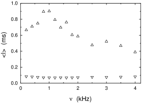
FIG. 1.: Mean lengths of the chaotic $(\triangle)$ and the regular $(\nabla)$ phases vs. modulation frequency.

FIG. 2.: (a) Probability distribution of the chaotic lengths for $\nu=\nu_{max}$. The full line indicates the exponential background. (b) Difference between the total probability and the exponential background taken from (a).

The influence of modulation frequency shows up in the duration of regular and chaotic phases (cf. fig.1). We found that the mean length of the regular state is not affected by the modulation. The mean chaotic length shows a distinct maximum at $\nu_{max}=1\mbox{kHz}$, which means that the reinjection from the chaotic to the regular state becomes less probable. At $\nu_{max}$ the mean return time, i.e. the sum of the two lengths, is of the order of the modulation period, which is a prerequisite for the occurrence of stochastic resonance.

Signatures of stochastic resonance could be observed in the distribution of the durations of the chaotic phase, i.e. the residence time distribution. Without modulation one would obtain an exponential decay, caused by the uniform reinjection from the chaotic to the regular state. With modulation there appears a structure on top of this background, which represents a typical feature of stochastic resonance [6]. The distribution at $\nu_{max}$ is plotted in fig. 2(a). The exponential background resulting from the intermittent dynamics is larger than in conventional stochastic resonance. Figure 2(b) shows the distribution after having subtracted this background. The distance between the peaks is equal to the modulation period $T_{m}$, as expected from theory. Since our system is strongly asymmetric the first peak is not located at exactly half the period but shifted towards a higher value.

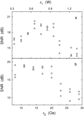
FIG. 3.: Signal–to–noise ratio vs. the bifurcation parameters $\varepsilon_{1}=P_{c}-P$ (a) and $\varepsilon_{2}=H_{c}-H$ (b) for various modulation frequencies ( $\Box\,1.0\mbox{kHz},$ $\circ\,5.0\mbox{kHz},$ $\triangle\,10.0\mbox{kHz}$ ).

Stochastic resonance was originally defined by an increase of the signal–to–noise ratio with increasing noise strength. In our experiments we have two possibilities to change the internal ”deterministic noise level”. At the bifurcation point ($H=H_{c}$, $P=P_{c}$) the regular state is marginally stable. With increasing bifurcation parameters $\varepsilon_{1}=P_{c}-P$ and $\varepsilon_{2}=H_{c}-H$ [9] the switching rate between regular and chaotic states increases and hence the internal noise level, too. If we take, as usual, the amplitude ratio between peak and background of the Fourier spectrum as a definition of the signal–to–noise ratio, we observe a maximum on variation of the static magnetic field or the microwave power. Figure 3 shows the results for several modulation frequencies on a logarithmic scale. Distinct resonance phenomena can be seen in both the field and power dependences.

III Theoretical model and simulations

Far above the Suhl threshold an approach from first principles has turned out to be extremely complicated [11]. Thus we adopt a phenomenological description in terms of simple mathematical model systems, which have proven to be fruitful in diverse problems of nonlinear dynamics. In order to develop a theoretical explanation for the residence time distribution we propose a time dependent one–dimensional map which can be treated analytically.

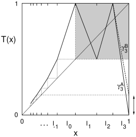
FIG. 4.: Piecewise linear map $x_{n+1}=T(x_{n})$. The broken line in $I_{3}$ and the double arrow show the time dependent modulation. The shaded box in the upper right corner indicates the region of the chaotic repeller.

This map generates a regular phase via an inverse pitchfork bifurcation and a chaotic phase via a chaotic repeller (cf. fig.4). We adopt a piecewise linear model with slopes $\gamma_{l}$ on the intervals $I_{l}$ to keep the analysis entirely analytical [14]. A periodic modulation with period $n_{p}$ is included via the time dependence of the slope in the right–hand interval $I_{3}$. For simplicity we confine ourself to the case where the slope $\gamma_{3}$ changes between two different values $\gamma_{3}^{A}$ and $\gamma_{3}^{B}$ every $(n_{p}/2)^{th}$ time step. Let $\rho_{l}(n)$ denote the probability density for a trajectory hitting the interval $I_{l}$ at time $n$. It is periodic in time with period $n_{p}$ but attains a constant value on each interval, since the model maps intervals on intervals (Markov map). Furthermore let $S_{k}(n)\subseteq I_{0}$ denote those phase space points which stay exactly $k$ time steps in the chaotic region $I_{1}\cup I_{2}\cup I_{3}$ if the initial phase of the modulation is $n$, and denote the size of this set by $\lambda(S_{k}(n))$. Then $\rho_{0}(n)\lambda(S_{k}(n))$ gives the probability that at phase $n$ of the modulation a chaotic burst of length $k$ occurs. Hence by averaging over the initial phase we obtain the desired distribution of residence times

$$N_{k}=\frac{1}{n_{p}\bar{\rho}_{0}\lambda(I_{0})}\sum_{n=0}^{n_{p}-1}\rho_{0}(n)\lambda(S_{k}(n))\quad,$$ (1)

where $\bar{\rho}_{0}$ denotes the average of $\rho_{0}(n)$ over one period. The structure of the distribution is determined by the time dependence of the density as well as by the time dependence of $S_{k}(n)$. The size of $S_{k}(n)$ can be expressed by the (static) escape rates of the chaotic repeller [15]. Using the abbreviation

$$p_{k}(n)=\left\{\begin{array}[]{lcl}p_{A}&:=&1/|\gamma_{1}|+1/|\gamma_{2}|+1/|\gamma_{3}^{A}|\\ &\mbox{if}&(k+n)|\mbox{mod }n_{p}<n_{p}/2\\ p_{B}&:=&1/|\gamma_{1}|+1/|\gamma_{2}|+1/|\gamma_{3}^{B}|\\ &\mbox{if}&(k+n)|\mbox{mod }n_{p}\geq n_{p}/2\end{array}\right.\quad,$$ (2)

a geometrical consideration yields

$$\lambda(S_{k}(n))=\lambda(I_{0})\prod_{i=1}^{k-1}p_{i}(n)\cdot(1-p_{k}(n))\quad.$$ (3)

The density $\rho_{0}(n)$ can in principle be evaluated, too. But to leading order in the modulation amplitude it remains time independent $\rho_{0}(n)\simeq\bar{\rho}_{0}$. This implies that the properties of the regular phase are not affected by the modulation, which is in accordance with our experimental observation. With eq.(3) the distribution (1) reads

$$N_{k}\simeq\frac{1}{n_{p}}\sum_{n=0}^{n_{p}-1}\prod_{i=1}^{k-1}p_{i}(n)\cdot(1-p_{k}(n))\quad.$$ (4)

Its structure is entirely determined by the time dependence of the escape rate and does not depend on details of the intermittency mechanism. Expression (4) is evaluated by combinatorics. In the case of large period $n_{p}\gg 1$ the distribution becomes quasi–continuous

$$N_{k}\simeq\exp(-\sigma k/n_{p})\left\{\begin{array}[]{ll}f_{-}(x),&0\leq x<1/2\\ f_{+}(x),&1/2\leq x<1\end{array}\right.\quad,$$ (5)

where $x=k/n_{p}|\mbox{mod }1$ denotes the fractional part of the chaotic length with respect to the modulation period. Expression (5) reflects an exponential decay of the distribution with rate $\sigma:=n_{p}[1-(p_{A}+p_{B})/2]$ and a superstructure of period $n_{p}$ (cf. fig.5), which is explicitly given by

$$f_{\pm}(1/2\pm z):=2z\sigma\cosh[\delta(1/2-z)]$$ (6)

$$\pm 2z\delta\sinh[\delta(1/2-z)]+2\sigma/\delta\sinh[\delta(1/2-z)]\quad.$$ (7)

Here $\delta:=(p_{B}-p_{A})n_{p}/2$ represents the amplitude of the modulation.

In addition to our analytical results we have performed computer simulations using a one–dimensional map like fig. 4 but with the left–hand part being replaced by a cubic function. The time dependence was introduced by modulation of the right–hand maximum. From the time series we evaluated the distribution of the residence times which are shown in fig. 5. Like for the analytical results we found an exponential decay modulated periodically with the period of the forcing. In this case, like for the ferromagnetic resonance experiments, a large exponential background occurs which is caused by the internal chaotic dynamics, i.e. the ”deterministic noise level”. The coincidence is even more convincing when keeping in mind that the analytical prediction and the simulation have been obtained from different maps and different modulation mechanisms.

FIG. 5.: Distribution of chaotic lengths. Analytical result (solid line) and simulation.

IV Conclusions

We have reported on the experimental realization of stochastic resonance in ferromagnetic resonance experiments beyond the Suhl threshold. In contrast to conventional stochastic resonance we used the interplay between the intrinsic chaotic dynamics in an intermittent parameter region and an external periodic modulation for the realization of noise–free stochastic resonance. Nevertheless the signal–to–noise ratio and the residence time distributions show exactly the same characteristic behaviour as in conventional stochastic resonance. We were able to explain these features in terms of a one–dimensional intermittent map. An analytical expression for the residence time distribution was derived and compared to results from computer simulations. Both the quantitative agreement between theoretical calculations and simulations, and the qualitative coincidence with the experimental result demonstrates the universality of these features. We expect that noise–free stochastic resonance will be realized in many other physical or technical applications in the near future.

V Acknowledgements

We thank Franz–Josef Elmer and Janusz Hołyst for helpful and interesting discussions. This project of SFB 185 ”Nichtlineare Dynamik” was partly financed by special funds of the Deutsche Forschungsgemeinschaft.

REFERENCES

- [1] R. Benzi, A. Sutera, and A. Vulpiani, J. Phys. A 14, L453 (1981).
- [2] F. Moss, A. Bulsara, and M. F. Shlesinger (eds.), J. Stat. Phys. 70, 1-512 (1993).
- [3] F. Moss, D. Pierson, and D. O’Gorman, Int. J. Bif. and Chaos 4, 1383 (1994).
- [4] R. Mannella, P. V. E. McClintock, and A. Bulsara (eds.), Nuovo Cimento D 17, ser. 1, nos. 7–8 (1995).
- [5] H. A. Kramers, Physica 7, 284 (1940).
- [6] T. Zhou, F. Moss, and P. Jung, Phys. Rev. A 42, 3161 (1990).
- [7] V. S. Anishchenko, A. B. Neiman, and M. A. Safanova, J. Stat. Phys. 70, 183 (1993).
- [8] F. Rödelsperger, Chaos und Spinwelleninstabilitäten (Harri Deutsch, Thun, 1994).
- [9] T. Bernard, R. Henn, W. Just, E. Reibold, F. Rödelsperger, and H. Benner, in Nonlinear Microwave Signal Processing: Towards a New Range of Devices, edited by R. Marcelli (Kluwer Acad. Publ., Dordrecht, 1996), p. 381–408.
- [10] R. W. Damon, in Magnetism, edited by G. T. Rado and H. Suhl (Academic Publ., New York, 1963), Vol. 1, p. 551ff.
- [11] H. Benner, F. Rödelsperger, and G. Wiese, in Nonlinear Dynamics in Solids, edited by H. Thomas (Springer, Berlin-Heidelberg, 1992), p. 129–155.
- [12] P. E. Wigen (ed.), Nonlinear Phenomena and Chaos in Magnetic Materials, World Scientific, Singapore (1994).
- [13] H. Suhl, J. Phys. Chem. Sol. 1, 209 (1957).
- [14] K. Shobu, T. Ose, and H. Mori, Prog. Theor. Phys. 71, 458 (1984).
- [15] T. Bohr and D. Rand, Physica D 25, 387 (1987).