On the Collective Motion
in Globally Coupled Chaotic Systems

Abstract

A mean–field formulation is used to investigate the bifurcation diagram for globally coupled tent maps by means of an analytical approach. It is shown that the period doubling sequence of the single site map induces a continuous family of periodic states in the coupled system. This type of collective motion breaks the ergodicity of the coupled map lattice. The stability analysis suggests that these states are stable for weak coupling strength but opens the possibility for more complicated types of motion in the regime of moderate coupling.

PACS No.:	05.45
Keywords:	Coupled map lattice, Synchronization
Running title:	Globally Coupled Chaotic Systems
Submitted to:	Phys. Rep.

1 Introduction

Despite the deep insight which has been gained into the dynamics of low dimensional chaotic systems and the sophisticated methods that have been developed for its analysis (cf.[1, 2]) there is a tremendous lack in the understanding of the influence of irregular motion on high dimensional dynamics. The failure is twofold. On the one hand it is not quite clear what kind of quantities are suitable for the characterization of chaotic motion in extended systems. On the other hand there is no common sense what kind of model systems capture the relevant features of chaotic motion in high dimensional phase spaces. Concerning the second problem systems of coupled maps have been proposed as suitable models [3] because of the simplicity of numerical simulations and of the fact that maps have proven as reasonable models for the investigation of low dimensional chaos. Although there does not exists a satisfactory derivation of coupled map lattices form physically sound equations of motion a rough estimate suggests [4] that they capture important features of realistic systems. In addition to a pure numerical simulation, analytical and even rigorous approaches have been applied successfully to simple coupled map lattices. Especially it has been shown that for rapidly decreasing interaction between the different lattices sites the hyperbolic property of the local dynamics is inherited to the coupled system, so that the space–time correlations decrease exponentially [5, 6]. This mixing property is sometimes used as an operating definition for space–time chaos although it does not seem to be fully satisfactory. It has been suggested that a breakdown of this regime can be understood in terms of phase transitions in the two dimensional spin lattice which serves as a symbolic dynamics [7].

In order to contribute by means of an analytical approach to the problem how chaos influences the motion in high dimensional phase spaces I will consider in this article a rather simple but nontrival coupled map lattice. For that purpose tent maps are chosen, as they have nontrivial features concerning their bifurcation scenario, their symbolic dynamics and their spectral properties but allow for an analytical treatment (cf. [8]). For the coupling mechanism an all to all interaction is the simplest choice so that one ends up with

$$x_{n+1}^{(\nu)} = \left(1-\epsilon\right)f\left(x_{n}^{(\nu)}\right)+\epsilon h_{n}=:T_{n}\left(x_{n}^{(\nu)}\right)$$ (1)

$$h_{n} := \frac{1}{N}\sum_{\mu=0}^{N-1}f\left(x_{n}^{(\mu)}\right)$$ (2)

$$f(x) := 1-a|x|\quad.$$ (3)

Here $N$ denotes the system size and we will dwell on the limit of large system size in the sequel. A superficial inspection of the central limit theorem together with the chaotic properties of the local dynamics would suggest that global quantities like the coupling field $h_{n}$ possess fluctuations which decrease as $N^{-1/2}$ with the system size. But such a property requires the factorization of the spatial correlation function at different sites (cf. [9]) and is in this sense equivalent to the mixing property referred above. It may be violated due to the infinite range of coupling, so that global quantities obey a nontrivial dynamics even in the limit of infinite system size [10]. It has been suggested that the occurence of such a kind of motion, which corresponds to a partial synchronization in the extended system, is related to the nonhyperbolic properties of the local dynamics [11]. For the simple model system (1)–(3) I want to investigate how such a kind of motion occurs.

For that purpose a mean–field like approach is used [12]. To keep the presentation self–contained and to set some notations this formulation will be recapitulated in section 2. With its help the bifurcation behaviour of periodic densities is analysed in section 3. The highly nontrivial aspect of the stability of these solutions is addressed in section 4.

2 Mean–field formulation

The value of the coupling field (2) is solely determined by the ”one–site” density

$$\rho_{n}(x):=\frac{1}{N}\sum_{\mu=0}^{N-1}\delta\left(x-x_{n}^{(\mu)}\right)$$ (4)

by dint of the relation

$$h_{n}=\int f(x)\rho_{n}(x)\,dx\quad.$$ (5)

If one recalls that the dynamics is governed by the effective map $T_{n}$ then the time evolution of the density (4) is given by

$$\rho_{n+1}(x)=\int\delta\left(x-T_{n}(y)\right)\rho_{n}(y)\,dy=:{\cal L}_{n}\rho_{n}(x)$$ (6)

where the map $T_{n}$ depends itself on the density (cf. eqs.(1), (5)). In this respect eq.(6) constitutes a nonlinear evolution equation for the ”one–site” density (4). It should be stressed that this expression is an exact consequence of the full evolution equation (1) as long as the density takes the form (4). In additon the system size does not enter the formulation in an explicit way.

It is supposed that the limit of infinite system size can be performed in such a way that instead of the special form (4) every integrable density is accessible during the evolution. Although this limit, understood in the weak sense, seems to be difficult to justify on a rigorous basis this assumption is highly plausible on physical grounds and can be supported by numerical simulations. By this assumption those transients which increase with the system size are turned into stable solutions of the mean–field description. Hence the stationary solutions of eq.(6) capture also the transient behaviour which becomes quasi–stationary in the limit of large system size and which governs the dynamics of large systems on accessible time scales.

The density (4) allows for the computation of any globally averaged quantity. In addition it has been demonstrated [13] that in cases where the the mean–field dynamics (6) converges to a stable solution, the correlation properties between different sites can be obtained from the ”one–site” density also.

3 Periodic Densities

We are going to construct periodic solutions $\rho_{0},\ldots,\rho_{p-1}$, $\rho_{p}=\rho_{0}$ of the evolution equation (6) by generalizing some ideas of [14]. For reasons that will become obvious in the sequel we consider periods $p=2^{M}$. Eq.(4) tells us that $\rho_{0}$ is determined by an invariant density of the map

$$\left(T_{p-1}\circ\ldots\circ T_{0}\right)(x)=\eta_{p-1}-a_{red}|\eta_{p-2}-\ldots-a_{red}|\eta_{0}-a_{red}|x||\ldots|\quad.$$ (7)

Here the abbreviations

$$a_{red}:=(1-\epsilon)a,\quad\eta_{n}:=1-\epsilon a\int|x|\rho_{n}(x)\,dx$$ (8)

have been introduced. $\eta_{n}$ is positive as long as the coupling strength satisfies $\epsilon<1$. We further note the trivial fact that every mean–field map $T_{i}(x)=\eta_{i}-a_{red}|x|$ is topological equivalent to a single tent map with a reduced parameter

$$F(z)=1-a_{red}|z|$$ (9)

by a linear coordinate transformation $x=\eta_{i}z$.

Let us first consider the simple case that all parameters (8) are equal $\eta_{0}=\ldots=\eta_{p}=\eta_{*}$. The $p^{th.}$ iterate of the map (9) admits of $p$ different ergodic components for $\sqrt[2p]{2}<a_{red}<\sqrt[p]{2}$. They correspond to the $p$–band chaos in the tent map. Let $\nu_{i}(x),i=0,\ldots,p-1$ denote the different normalized ergodic absolutely continuous distributions and let $\nu_{0}$ denote that ergodic component which contains the critical point $z=0$. They obey the Frobenius–Perron equation which reads $\nu_{i+1}(x/\eta_{*})={\cal L}_{*}\nu_{i}(x/\eta_{*})$. For $1\leq i\leq p-1$ it just leads to an affine transformation of the distributions $\nu_{i}$. The density

$$\rho_{0}(x):=\sum_{i=0}^{p-1}\frac{1}{2^{M}}\frac{1}{\eta_{*}}\nu_{i}\left(\frac{x}{\eta_{*}}\right)\quad.$$ (10)

constitutes by construction a $p$ periodic orbit of eq.(4) which in fact is a fixed point. Finally the free parameter $\eta_{*}$ is determined by the relation (8)

$$\eta_{*}=1-\epsilon\eta_{*}\sum_{i=0}^{p-1}\frac{1}{2^{M}}\int|z|\nu_{i}(z)\,dz$$ (11)

where it is worth to mention again that the distributions $\nu_{i}$ depend only on $a_{red}$ by definition. The meaning of this fixed point solution is quite simple. Every periodic chaotic band contributes to the density (10) in such a way that the time dependencies cancel each other exactly. Finally let us denote for later reference by $\sigma_{i}$ the symbol sequence of the critical point that means $\sigma_{i}=\mbox{sgn}(T^{i+1}_{*}(0))$.

We continue our construction of a continuous family of periodic solutions by giving the different ergodic components different weight factors. For that purpose one has to show that the components are not destroyed if the parameters $\eta_{n}$ are not equal. In fact as sketched in Fig. 1 the change of these quantities will lead only to an affine transformation of the different components but not to topological changes.

Figure 1: Diagrammatic view of the second iterate $T_{1}\circ T_{0}$ for $\sqrt[4]{2}<a_{red}<\sqrt{2}$ and two different choices of parameters $\eta_{i}$.

To make this statement explicit consider a $p$ periodic sequence of parameters $\eta_{i}$ close to the value $\eta_{*}$ mentioned above. Fix a neighbourhood of the critical point $x=0$ that contains the support of the former ergodic component. As the finite itinerary of the critical point $\sigma_{0},\ldots,\sigma_{p}$ is unaltered for $\eta_{i}$ sufficiently close to $\eta_{*}$ the iterated map (7) on this neighbourhood reads

$$\left(T_{p-1}\circ\ldots\circ T_{0}\right)(x)=\sum_{l=0}^{p-1}(-a_{red})^{p-l-1}\cdot\prod_{k=l}^{p-2}\sigma_{k}\cdot\eta_{l}+(-a_{red})^{p-1}\cdot\prod_{k=0}^{p-2}\sigma_{k}\cdot|x|\quad.$$ (12)

Since this expression is in a neighbourhood of the critical point topological equivalent to the $p^{th}$ iterate of the single tent map (9), eq.(12) admits of an ergodic component $\tilde{\nu}_{0}(x)$. It is given in terms of the corresponding ergodic component $\nu_{0}$ of the single map by

$$\tilde{\nu}_{0}(x)=\frac{1}{\Gamma}\nu_{0}\left(\frac{x}{\Gamma}\right)$$ (13)

where the scaling factor $\Gamma$ follows from the linear conjugacy to be

$$\Gamma\sum_{l=0}^{p-1}(-a_{red})^{p-l-1}\cdot\prod_{k=l}^{p-2}\sigma_{k}=\sum_{l=0}^{p-1}(-a_{red})^{p-l-1}\cdot\prod_{k=l}^{p-2}\sigma_{k}\cdot\eta_{l}\quad.$$ (14)

By construction the sequence of densities $\tilde{\nu}_{i+1}:={\cal L}_{i}\tilde{\nu}_{i}$ is periodic with period $p$. In view of the fact that the mean–field map $T_{i}$ is conjugate to the single tent map (9), and that the former acts as an affine transformation for $\eta_{i}$ sufficiently close to $\eta_{*}$, it is a simple task to express the densites $\tilde{\nu}_{i}$ in terms of the ergodic components $\nu_{i}$ of the single map

$$\tilde{\nu}_{i}(x) = \frac{1}{\Gamma}\nu_{i}\left(\frac{x-\delta_{i}}{\Gamma}\right)$$ (15)

$$\delta_{i} := \sum_{l=0}^{i-1}(-a_{red})^{i-l-1}\cdot\prod_{k=l}^{i-2}\sigma_{k}\cdot\left(\eta_{l}-\Gamma\right)\quad.$$ (16)

Eq.(15) just states that the densities $\tilde{\nu}_{i}$ follow by an affine transformation from the ergodic components $\nu_{i}$. In order that this representation is valid it is necessary, that the support of these densities is not shifted across the critical point, that means $\delta_{i}$ has to be sufficiently small. But from eqs.(14) and (16) it is obvious that this property holds for $\eta_{i}$ sufficiently close to $\eta_{*}$. Now by construction the $p$ periodic convex sum

$$\rho_{n}(x)=\sum_{i=0}^{p-1}\alpha_{n+i}\tilde{\nu}_{i}(x),\quad\alpha_{n+p}=\alpha_{n}\in[0,1],\quad\sum_{k=0}^{p-1}\alpha_{k}=1$$ (17)

satisfies eq.(6). It remains to show that the weights $\alpha_{i}$ can be chosen in such a way that the self–consistency condition (8) is valid. For that purpose one inserts the density (17) into eq.(8) and obtains

$$\eta_{n}=1-\epsilon a\sum_{i=0}^{p-1}\alpha_{n+i}\left(\Gamma\zeta_{i}+\sigma_{i-1}\delta_{i}\right)\quad.$$ (18)

Here we have expressed the integrals in terms of the densities $\nu_{i}$ of the single map and have used the abbreviation

$$\zeta_{i}:=\int|z|\nu_{i}(z)\,dz\quad.$$ (19)

But now eqs.(18) and the definitions (14) and (16) yield a system of $p$ linear equations for the $p$ coefficients $\eta_{n}$ if one considers the weights $\alpha_{i}$ as given. The solution of this system completes the construction of the periodic density. It is completely given in terms of the densities of the single map (9).

Hence one has found a continuous family of $p=2^{M}$ periodic solutions for $\sqrt[2p]{2}<a_{red}<\sqrt[p]{2}$ which emerges by attributing slightly different weights to the different ergodic components of the iterated mean–field map (cf. eq.(17)). Fig. 2 summarizes this result in a partial bifurcation diagram.

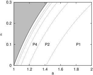
Figure 2: Bifurcation diagram for globally coupled tent maps. $Pn$ denotes the region where a continuous family of $n$ periodic densities exists. The shaded area indicates the region where asymptotic periodicity gets lost.

The period doubling of chaotic attractors of the single map translates into the bifurcation of periodic densities of the coupled system. At each bifurcation line the period $p$ family of densities splits into a period $2p$ family of densities. As was already mentioned in [15] at $a_{red}=1$ asymptotic periodicty gets lost. In addition the bifurcation at $a_{red}=\sqrt{2}$ has been observed in numerical simulations some time ago [12].

I have yet not claimed that the periodic densities are stable. One might argue that on physical grouds these solutions are stable, as the ergodic components are preserved in the coupled map lattice. But as was already mentioned in [13] the problem of stability turns out to be highly nontrivial. Furthermore in numerical simulations of finite lattices one observes additonal oscillations [16] which cannot be attributed to the period doubling scenario. Before I turn to the discussion of the stability let me demonstrate by means of a numerical approach that the densities might be stable at least for small coupling. For that purpose simulations of eqs.(1)–(3) have been performed for parameter values within the period 2 and 4 window. For different lattice sizes one finds a corresponding periodic motion in the coupling field on which a ”noisy” component is superimposed. In order to check whether this component is a finite size effect the mean square deviation, that means the second cumulant of the $p^{th}$ iterate of $h_{n}$, has been analysed in dependence on the system size (cf. Fig.3).

Figure 3: Mean square deviation $\Delta$ of the second respectively fourth iterate of the coupling field $h_{n}$ for $\epsilon=0.1$ and two values of $a_{red}$ in dependence on the system size.

The behaviour according to the central limit theorem suggests that the nonperiodic component is a finite size effect and that these periodic states are dynamically stable. But the numerical values of the periodic density depend on the initial condition. Hence the latter determines which member of the continous family of periodic densities is selected as the stationary state.

4 Stability Analysis

The linear stability analysis of the equation of motion (6) faces the problem that the densities are in general not smooth functions. Following the ideas of [13] this equation takes a somewhat simpler form if one restricts the analysis to the case of densities which are made of a countable infinite number of step functions

$$\rho_{n}(x)=\sum_{j=0}b_{n}^{j}\Theta\left(c_{n}^{j}-x\right)\quad.$$ (20)

Due to the piecewise linear shape of the tent map this form is preserved during the evolution. Then eqs.(5), (6) read (cf. [17])

$$b_{n+1}^{0} = \frac{1}{a_{red}}\sum_{j=0}b_{n}^{j}\left[\mbox{sgn}(c_{n}^{j})+1\right]$$ (21)

$$b_{n+1}^{j+1} = -\frac{1}{a_{red}}b_{n}^{j}\mbox{sgn}(c_{n}^{j})$$ (22)

$$c_{n+1}^{0} = T_{n}(0)$$ (23)

$$c_{n+1}^{j+1} = T_{n}\left(c_{n}^{j}\right)$$ (24)

$$T_{n}(x) = 1-\epsilon+\epsilon h_{n}-a_{red}|x|$$ (25)

$$h_{n} = 1-\frac{a}{2}\sum_{j=0}b_{n}^{j}c_{n}^{j}|c_{n}^{j}|\quad.$$ (26)

We will consider only the stability properties of the fixed point solution (10) in the sequel. In terms of the representation (20) this solution is obtained from eqs.(21)–(24)

$$b_{*}^{j} = \left(-\frac{1}{a_{red}}\right)^{j}b_{*}^{0}\prod_{k=0}^{j-1}\sigma_{k}$$ (27)

$$c_{*}^{j} = T_{*}^{j+1}(0)$$ (28)

$$1 = b_{*}^{0}\sum_{j=0}\left(-\frac{1}{a_{red}}\right)^{j}c_{*}^{j}\prod_{k=0}^{j-1}\sigma_{k}$$ (29)

where again $\sigma_{j}:=\mbox{sgn}(c_{*}^{j})$ denotes the symbol sequence of the critical point. To investigate the stability properties of this solution let us consider the eigenvalue problem that emerges from the formal linearization of the evolution equations (21)–(26)

$$\lambda\beta^{0} = \frac{1}{a_{red}}\sum_{j=0}\beta^{j}(\sigma_{j}+1)$$ (30)

$$\lambda\beta^{j+1} = -\frac{1}{a_{red}}\beta^{j}\sigma_{j}$$ (31)

$$\lambda\gamma^{0} = \epsilon\delta h$$ (32)

$$\lambda\gamma^{j+1} = \epsilon\delta h-a_{red}\gamma^{j}\sigma_{j}$$ (33)

$$\delta h := -\frac{a}{2}\sum_{j=0}\left(c_{*}^{j}|c_{*}^{j}|\beta^{j}+2b_{*}^{j}|c_{*}^{j}|\gamma^{j}\right)\quad.$$ (34)

Since these equations decouple the eigenvalue problem can be analysed on both invariant subspaces separately.

With the solution of eq.(31)

$$\beta^{j}=\left(-\frac{1}{a_{red}\lambda}\right)^{j}\beta^{0}\prod_{k=0}^{j-1}\sigma_{k}$$ (35)

eq.(30) yields the characteristic equation

$$0=\left(1-z\right)\sum_{j=0}(-z)^{j}\prod_{k=0}^{j-1}\sigma_{k},\quad z:=\frac{1}{a_{red}\lambda}\quad.$$ (36)

The sum on the right hand side is just the $\lambda$–expansion and yields the spectrum of the Frobenius–Perron operator of the fixed point map $T_{*}$ [8]. Hence the spectrum is contained within the unit circle and the eigendirections belong to the center–stable manifold of the fixed point density. Obviously there occurs a doubly degenerated eigenvalue $\lambda=1$. It is caused by two constants of motion $\sum_{j}b_{n}^{j}=0$, $\sum_{j}b_{n}^{j}c_{n}^{j}=1$ of eqs.(21)–(26) which reflect the normalization of the density and the boundary condition $\rho_{n}(-1)=0$.

Using the solution of eqs.(32), (33)

$$\gamma^{j}=\sum_{l=0}^{j}\prod_{k=1}^{l}\left(-\frac{a_{red}}{\lambda}\sigma_{j-k}\right)\cdot\frac{\epsilon\delta h}{\lambda}$$ (37)

eq.(34) yields for $\beta^{j}\equiv 0$ the characteristic equation

$$1=-\frac{a\epsilon}{\lambda}\sum_{l=0}\left(-\frac{a_{red}}{\lambda}\right)^{l}\sum_{j=l}b_{*}^{j}|c_{*}^{j}|\prod_{k=1}^{l}\sigma^{j-k}\quad.$$ (38)

If one takes the representation (27) of the fixed point into account one ends up with

$$1=-\frac{a\epsilon}{\lambda}\sum_{l=0}\kappa_{l}\left(-\frac{1}{\lambda}\right)^{l}$$ (39)

where the coefficients are given by

$$\kappa_{l}:=b_{*}^{0}\sum_{j=0}\left(-\frac{1}{a_{red}}\right)^{j}|c_{*}^{j+l}|\prod_{k=0}^{j-1}\sigma_{k}\quad.$$ (40)

Although one has obtained a quite simple expression which can be evaluated by means of a numerical approach it seems to be difficult to make general statements about the solutions of eq.(40) respectively its analytical continuation. But if one restricts to the simple case that the itinerary terminates in the fixed point of the map $T_{*}$, that means $|c_{*}^{l}|=c_{F}$, $l\geq l_{0}$, then the coefficients obey

$$\alpha_{l}=b_{*}^{0}c_{F}\sum_{j=0}\left(-\frac{1}{a_{red}}\right)^{j}\prod_{k=0}^{j-1}\sigma^{k}=0,\quad l\geq l_{0}\quad.$$ (41)

To establish this identity one has used the fact that the sum represents the $\lambda$–expansion of the fixed point map $T_{*}$ and that its Frobenius–Perron operator admits of the eigenvalue $\lambda=1$ [8]. Hence the characteristic equation (39) reduces to a polynomial which yields for sufficiently small coupling only eigenvalues within the unit circle.

5 Discussion

The bifurcation diagram depicted in Fig. 2 summarizes main results of this article. It provides a foliation of the region of asymptotic periodicity $a_{red}>1$. In each region a continuous family of periodic states, which is generated by the different ergodic components of the iterated tent map, accounts for the time dependency of the stationary solution.

The stability analysis suggests that these states are stable at least for small coupling strength $\epsilon$. But there are several limitations in this analysis. For the stability of the fixed point density the estimates presented in section 4 are not uniformly valid in the parameter space and the problem whether stability is attained on a parameter set of sufficiently large measure is not solved. However numerical simulations and a numerical analysis of the eigenvalue equations (30)–(34) [17] suggest stabilty for small coupling. In addition one should recall that the discussion of stability presented above was based on a formal linearization of the evolution equation. Such a procedure takes deviations of the parameters $c^{j}$ with equal weight into account. This approach seems to overestimate the effect of these deviations on the density (20) since the coefficients $b^{j}$ decay exponentially. Hence one has to specify the space on which the eigenvalue problem has to be treated which may restrict the spectrum to a few relevant eigenvalues (cf. e.g. [18] for such a phenomenon in the context of the Frobenius–Perron operator). Despite these shortcommings the approach presented here might be a basis for further investigations.

The periodic states investigated in this article explain in a clear fashion the time dependence of globally averaged quantities. Therefore one mechanism for time fluctuations in globally averaged quantities seems to be well understood. But numerical simulations of coupled tent maps show additional quasiperiodic solutions [16]. The explanation of this kind of collective motion which resembles in some respect a Hopf bifurcation seems to be one challenge for the further research in this field. In addition it might be this kind of motion which appears in the frequently analysed case of coupled logistic maps.

The feasibility of analytical computations on piecewise linear map lattices make these kind of models suitable for studying the influence of chaotic motion in high dimensional systems. Even the apparently simple model treated in this article shows several unexpected features and it is far from being solved completely. Other problems may be attacked by this kind of model also, e.g. the effect of a long but not infinte range of coupling in connection with the validity of a mean–field treatment, or the construction of the symbolic dynamics and the effect of pruning of symbol sequences. But these questions are left for future work.

References

- [1] J.-P.Eckmann and D.Ruelle, Rev. Mod. Phys. 57, 617 (1985).
- [2] J.Guckenheimer and P.Holmes, Nonlinear Oscillations, Dynamical Systems, and Bifurcations of Vector Fields, Applied Mathematical Sciences 42, Springer, New York, 1986.
- [3] K.Kaneko, Physica D 34, 1 (1989).
- [4] T.Yamada and H.Fujisaka, Prog. Theor. Phys. 72, 885 (1984).
- [5] L.A.Bunimovich and Ya.G.Sinai, Nonlin. 1, 491 (1988).
- [6] J.Bricmont and A.Kupiainen, Nonlin. 8, 379 (1995).
- [7] L.A.Bunimovich, Physica D 86, 248 (1995).
- [8] M.Dörfle, J. Stat. Phys. 40, 93 (1985).
- [9] M.Ding and L.T.Wille, Phys. Rev. E 48, R1605 (1993).
- [10] A.S.Pikovsky and J.Kurths, Phys. Rev. Lett. 72, 1644 (1994).
- [11] W.Just, Physica D 81, 317 (1995).
- [12] K.Kaneko, Physica D 55, 368 (1992).
- [13] S.V.Ershov and A.B.Potapov, Physica D 86, 523 (1995).
- [14] W.Just, J. Stat. Phys. 79, 429 (1995).
- [15] J.Losson, J.Milton and M.C.Mackey, Physica D 81, 177 (1995).
- [16] K.Kaneko, Physica D 86, 158 (1995).
- [17] S.Morita, Phys. Lett. A 211, 258 (1996).
- [18] W.C.Saphir and H.H.Hasegawa, Phys. Lett. A 171, 317 (1992).