Periodic Orbits, Breaktime and Localization

Abstract

The main goal of the present paper is to convince that it is feasible to construct a ‘periodic orbit theory’ of localization by extending the idea of classical action correlations. This possibility had been questioned by many researchers in the field of ‘Quantum Chaos’. Starting from the semiclassical trace formula, we formulate a quantal-classical duality relation that connects the spectral properties of the quantal spectrum to the statistical properties of lengths of periodic orbits. By identifying the classical correlation scale it is possible to extend the semiclassical theory of spectral statistics, in case of a complex systems, beyond the limitations that are implied by the diagonal approximation. We discuss the quantal dynamics of a particle in a disordered system. The various regimes are defined in terms of time-disorder ‘phase diagram’. As expected, the breaktime may be ‘disorder limited’ rather than ‘volume limited’, leading to localization if it is shorter than the ergodic time. Qualitative agreement with scaling theory of localization in one to three dimensions is demonstrated.

1 Introduction

Extending the semiclassical approach to spectral statistics beyond the diagonal approximation is presently one of the most vigorously pursued direction of research in “quantum chaos”. It is desirable to reach a semiclassical understanding of the long-time behavior also for disordered systems. They play a central role in condensed-matter as well as in mesoscopic physics. The introduction of semiclassical methods in the latter case is quite natural. It can be expected that a semiclassical insight into localization will, in turn, shed new light on semiclassical methods in general. The present paper is intended as a contribution towards this goal. It rests mainly on two previous observations: the connection between spectral correlations in the long-time regime and classical action-correlations [1], and the heuristic treatment of localization by Allen [2]. It turns out that the latter appears as a natural consequence of the former, once a disorder system is considered. An improved qualitative picture of spectral statistics follows, expressed in the form of ‘time-disorder’ diagram. Furthermore, the present formulation paves the way towards a quantitative account in terms of the spectral form factor.

There are few time scales that are associated with the semiclassical approximation for the time-evolution of any observable. Such an approximation involves a double-summation over classical orbits. The purpose of the following paragraphs is to make a clear distinction between these various time scales. In particular we wish to clarify the ‘breaktime’ concept that plays a central role in our formulation. Initially the classical behavior is followed. One relevant time scale for the departure from the classical behavior is $t_{scl}$. By definition, when $t_{scl}<t$ deviations that are associated with the breakdown of the stationary phase approximation may show up. It has been argued [3] that $t_{scl}\sim\hbar^{-1/3}$. Further deviations from the leading order semiclassical expansion due to diffraction effects are discussed in [4]. One should be careful not to confuse these deviations, which are associated with the accuracy of the stationary phase approximation with the following discussion of the breaktime concept. It is assumed in the sequel that the leading order semiclassical formalism constitutes a qualitatively good approximation also for $t_{scl}{<}t$ in spite of these deviations.

Interference effects lead to further deviations from the classical behavior. Well isolated classical paths, for which the stationary phase approximation is completely accurate, still may give rise to either constructive or destructive interference effect. From now on we shall put the focus on the semiclassical computation of the spectral form factor [5], where the double-summation is over classical periodic orbits (POs). We shall disregard extremely short times, for which only few POs contribute, since for any generic chaotic system the POs proliferate exponentially with time. The simplest assumption would be that the interference contribution (off-diagonal terms) is self-averaged to zero. However, such an assumption would imply that the classical behavior is followed for arbitrarily long times. This is obviously not true. After a sufficiently long time the discrete nature of the energy spectrum becomes apparent, and the recurrent quasiperiodic nature of the dynamics is revealed. The breaktime $t^{*}$ is the time scale which is associated with the latter crossover. Neglecting the interference contribution for $t<t^{*}$ is known as the diagonal-approximation [5].

From semiclassical point of view the breaktime $t^{*}$ is related to the breakdown of the diagonal approximation. It has been conjectured that the breakdown of the diagonal approximation is a manifestation of classical action-correlations [1]. Else, if the actions were uncorrelated (Poisson statistics), then the off-diagonal (interference) contribution would be self-averaged to zero. Typically the breaktime $t^{*}$ is identified with the Heisenberg time $t_{H}=2\pi\hbar/\Delta E$, where $\Delta E$ is the average level spacing. The Heisenberg time is semiclassically much longer than the ‘log’ time $t_{E}\sim\ln(1/\hbar)$ over which classical orbits proliferates on the uncertainty scale. The latter time scale has no physical significance as far as the form factor is concerned. See also discussion after Eq.(12).

The breaktime which is determined by the Heisenberg uncertainty relation is volume dependent. However, for a disordered system the breaktime may be much shorter and volume-independent due to localization effect. The theory for this this ‘disordered limited’ rather than ‘volume limited’ breaktime constitutes the main theme of the present paper. Our approach to deal with disorder within the framework of the semiclassical approach constitutes a natural extension of previous attempts to integrate ‘mesoscopic physics’ with the so called field of ‘quantum chaos’. See [6] for review. Note that a naive semiclassical arguments can be used in order to estimate the breaktime and the localization length for 1D systems [7]. See the next section for further details. This argument, as it stands, cannot be extended to higher dimensions, which implies that a fundamentally different approach is needed. The same objection applies to a recent attempt to propose a periodic orbit theory for 1D localization [8]. In the latter reference the semiclassical argument for localization is based on proving exponentially-small sensitivity for change in boundary conditions. This is due to the fact that only exponentially small number of POs with $t{<}t_{H}$ hit the edges. The statement holds for $d{=}1$, where $t_{H}{\ll}t_{erg}$, but it fails in higher dimensions. Hence the necessary condition for having localization should be much weaker.

The plan of this paper is as follows. The expected results for the disordered limited breaktime, based on scaling theory of localization, are presented in Section 2. Our main goal is to re-derive these results from semiclassical consideration. In section 3, starting from the semiclassical trace formula (SCTF), we formulate a duality relation that connects the spectral properties of the quantal spectrum to the classical two-point statistics of the POs. In section 4 we identify the classical correlation scale. Then it is possible to extend the semiclassical theory of spectral statistics, in case of a complex systems, beyond the limitations that are implied by the diagonal approximation. In section 5 we demonstrate that a disorder limited breaktime is indeed a natural consequence of our formulation. The various time regimes for a particle in a disordered system are illustrated using a time-disorder ‘phase diagram’. Localization show-up if there is a disorder limited breaktime which is shorter than the ergodic time. Semiclassical interpretation for the existence of a critical and an ohmic regimes for 3D localization is also introduced. Finally, in section 6, we introduce a semiclassical approximation scheme for the form factor, that goes beyond the diagonal approximation. The limitations of this new scheme are pointed out.

Effects that are associated with the actual presence of a magnetic field are not considered in this paper, since the SCTF should be modified then. Still, for simplicity of presentation we cite for the form factor the GUE rather than the GOE result, and we disregard the effect of time reversal symmetry. A proper treatment of these details is quite obvious, and will appear in a future publication [9]. It is avoided here in order not to obscure the main point.

2 Breaktime for Disordered Systems

We consider a particle in a disordered potential. The classical dynamics is assumed to be diffusive. For concreteness we refer to a disordered billiard. The concept is defined below. It should be emphasized that we assume genuine disorder. Pseudo-random disorder, as well as spatial symmetries are out of the scope of our considerations.

A disordered billiard is a quasi $d$-dimensional structure that consists of connected chaotic cavities. Here we summarize the parameters that are associated with its definition. The billiard is embedded in $d_{0}$-dimensional space ($2\leq d_{0}$). It constitutes a $d$ dimensional structure of cells, (obviously $d\leq d_{0}$). Each cell, by itself, constitutes a chaotic cavity whose volume is roughly $\ell_{0}^{d_{0}}$. However, the cells are connected by small holes whose area is $a_{0}^{d_{0}{-}1}$ with $a_{0}\ll\ell_{0}$. The volume of the whole structure is $\Omega={\cal L}^{d}\ell_{0}^{d_{0}{-}d}$. Assuming a classical particle whose velocity is $v$, the average escape time out of a cell is $t_{0}\approx(\ell_{0}/v)\cdot(\ell_{0}/a_{0})^{d_{0}{-}1}$. The classical diffusion coefficient is ${\cal D}_{0}=\ell_{0}^{2}/t_{0}$. The classical diffusion law is $\langle(x-x_{0})^{2}\rangle={\cal D}_{0}t$ where $x_{0}$ is the location of an initial distribution.

The mass of the particle is $m$. Its De-Broglie wavelength $\lambda_{B}=\hbar/mv$ is assumed to be much shorter than $\ell_{0}$ as to allow (later) semiclassical considerations. Actually, in order to have non-trivial dynamical behavior $\lambda_{B}$ should be smaller or at most equal to $a_{0}$ (note the following definition of the dimensionless conductance). The mean energy level spacing is $\Delta E=2\pi\alpha^{-1}{\cdot}(\hbar^{d_{0}}/{\cal L}^{d})$ where $\alpha\sim\ell_{0}^{d_{0}{-}d}m^{d_{0}{-}1}v^{d_{0}{-}2}$. The Heisenberg time is $t_{H}=2\pi\hbar/\Delta E=\alpha{\cal L}^{d}/\hbar^{d_{0}{-}1}$ The dimensionless conductance $g_{0}$ on scale of one cell is defined as the ratio of the Thouless energy $2\pi\hbar/t_{0}$ to the level spacing $2\pi\hbar/t_{H}$. (for $t_{H}$ one should substitute here ${\cal L}=\ell_{0}$). Hence $g_{0}=(a_{0}/\lambda_{B})^{d_{0}{-}1}$ is simply related to the hole size. Out of the eight independent parameters $(d_{0},d,\ell_{0},a_{0},{\cal L},m,v,\hbar)$ there are actually only three dimensionless parameters which are relevant. Setting $t_{0}$ and $\ell_{0}$ to unity, these are $d$, $g_{0}$ and ${\cal L}$. All the results should be expressed using these parameters.

For a billiard system in $d$-dimension, whose volume is $\Omega$, the Heisenberg-time is given by the expression $t_{H}=\alpha\Omega/\hbar^{d{-}1}$. For the disordered billiard Heisenberg time can be expressed in terms of the unit-cell dimensionless conductance

$$t^{*}_{H}\ =\ \frac{2\pi\hbar}{\Delta E}\ =\ \alpha\frac{\Omega}{\hbar^{d_{0}{-}1}}\ =\ \left(\frac{{\cal L}}{\ell_{0}}\right)^{d}g_{0}t_{0}$$ (1)

The actual ‘disordered limited’ breaktime may be much shorter due to localization effect. Naive reasoning concerning wavepacket dynamics leads to the volume-independent estimate [7]

$$t^{*}\ =\ \frac{2\pi\hbar}{\Delta_{\xi}}\ =\ \alpha\frac{\xi^{d}}{\hbar^{d_{0}{-}1}}\ \ \ \ \ [\mbox{naive}]\ .$$ (2)

Here $\Delta_{\xi}$ is the effective level spacing within a volume $\xi^{d}$. Assuming that up to $t^{*}$ the spreading is diffusive-like, it follows that

$$\xi^{2}\ =\ {\cal D}_{0}\ t^{*}$$ (3)

Combining these two equations it has been argued [7] that for quasi one-dimensional structure ($d{=}1$) the localization length is $\xi{\sim}\alpha{\cal D}_{0}/\hbar^{d_{0}{-}1}$. In terms of the dimensionless conductance the result is $\xi{=}g_{0}\ell_{0}$ which corresponds to the breaktime

$$t^{*}\ =\ g_{0}^{2}\ t_{0}\ \ \ \ \ [\mbox{for}\ \ d{=}1]\ .$$ (4)

The above argument that relates $\xi$ and $t^{*}$ to the dimensionless conductance $g_{0}$ cannot be extended in case of $1{<}d$. This is due to the fact that (2) overestimates the breaktime. From scaling theory of localization [10] one obtains for $d{=}2$ the result $\xi{=}\mbox{e}^{g_{0}}\ell_{0}$ leading (via equation (3)) to

$$t^{*}\ =\ \mbox{e}^{2g_{0}}\ t_{0}\ \ \ \ \ [\mbox{for}\ \ d{=}2]\ .$$ (5)

For $d{=}3$ and $g{<}g_{c}$, where $g_{c}$ is the critical value of $g$, scaling theory predicts $\xi{=}|g{-}g_{c}|^{-\nu}\ell_{0}$, with $\nu{\approx}1/(d{-}2)$. Here the diffusive-like behavior up to $t^{*}$ is replaced by an anomalous scale-dependent diffusive behavior, leading to the relation $\xi^{d}{=}\ell_{0}^{d{-}2}{\cal D}_{0}t^{*}$ rather than (3), and hence

$$t^{*}\ =\ \frac{1}{|g_{0}-g_{c}|^{\nu d}}\ t_{0}\ \ \ \ \ [\mbox{for}\ \ d{=}3]\ .$$ (6)

It is easily verified that the naive formula (2) overestimates the actual breaktime by factor $g_{0}$ for both $d{=}2$ and $d{=}3$. We turn now to develop a semiclassical theory for the breaktime.

3 Quantal-Classical Duality

The Semiclassical trace formula (SCTF) [11] relates the quantal density of states to the classical density of periodic orbits (POs). The quantal spectrum $\{k_{n}\}$ for a simple billiard in $d$ dimensions is defined by the Helmholtz equation $(\nabla^{2}{+}k^{2})\psi=0$ with the appropriate boundary conditions. The corresponding quantal density is

$$\rho_{qm}(k)\equiv\sum_{n}2\pi\delta(k{-}k_{n})\ |_{osc}\ \ \ \ .$$ (7)

In order to facilitate the application of Fourier transform conventions a factor $2\pi$ has been incorporated and let $\rho(k){=}\rho(-k)$ for $k{<}0$. The subscript $osc$ implies that the averaged (smoothed) density of states is subtracted. This smooth component equals the corresponding Heisenberg length and is found via Weyl law, namely

$$L_{H}(k)\ =\ C_{d}\Omega\ k^{d{-}1}$$ (8)

where $\Omega$ is the volume of the billiard, and $C_{d}=(2^{d{-}2}\pi^{{d}/{2}{-}1}\Gamma({d}/{2}))^{-1}$. For billiard systems, actions lengths and times are trivially related by constant factors and therefore can be used interchangeably. In the sequel some of the formulas become more intelligible if one recalls that $L$ plays actually the role of the time. The classical spectrum $\{L_{j}\}$ consists of the lengths of the POs and their repetitions. The corresponding weighted density is

$$\rho_{cl}(L)\equiv\sum_{j}A_{j}\delta(L{-}L_{j})\ |_{osc}\ \ \ \ .$$ (9)

Here $A_{j}$ are the instability amplitudes. We note that for a simple chaotic billiard, due to ergodicity $K_{D}(L)\equiv\langle\sum_{j}|A_{j}|^{2}\delta(L{-}L_{j})\rangle\sim L$. The instability amplitudes decay exponentially with $L$, namely $|A_{j}|^{2}{\sim}L^{2}\exp(-\sigma L)$, where $\sigma$ is the Lyapunov exponent. Hence the density of POs grows exponentially as $\exp(\sigma L)/L$. with the above definitions the SCTF is simply

$$\rho_{qm}(k)\ \ =\ \ {\cal FT}\ \rho_{cl}(L)\ \ \ \ .$$ (10)

Where the notation ${\cal FT}$ is used in order to denote a Fourier transform. Both the SCTF and the statistical relation (11) that follows, reflect the idea that the quantal spectrum and the classical spectrum are two dual manifestations of the billiard boundary.

The two-points correlation function of the quantal spectrum is $R_{qm}(k,\epsilon)\equiv\langle\rho_{qm}(k)\rho_{qm}(k{+}\epsilon)\rangle$, where the angle brackets denote statistical averaging. The spectral form factor $K_{qm}(k,L)$ is its Fourier transform in the variable $\epsilon{\leadsto}L$. Due to the self correlations of the discrete energy spectrum $R_{qm}(\epsilon)$ is delta-peaked in its origin. As a consequence the asymptotic behavior of the spectral form factor is $K_{qm}(k,L)=L_{H}(k)$ for $L_{H}(k){\ll}L$. For a simple ballistic billiard the crossover to the asymptotic behavior occurs indeed at the Heisenberg time. The functional form of the crossover is described by Random Matrix Theory (RMT). For concreteness we cite the approximation $K_{qm}(k,L){=}\min(L,L_{H}(k))$. (Effect of symmetries is being ignored for sake of simplicity). In order to formulate a semiclassical theory for the form factor it is useful to define the two point correlation function of the classical spectrum $R_{cl}(x,L)\equiv\langle\rho_{cl}(L)\rho_{cl}(L{+}x)\rangle$. The corresponding form factor $K_{cl}(k,L)$ is obtained by Fourier transform in the variable $x{\leadsto}k$. It is straightforward to prove that due to the SCTF $R_{qm}(k,\epsilon)$ is related to $R_{cl}(x,L)$ by a double Fourier transform. Hence

$$K_{qm}(k,L)\ =\ K_{cl}(k,L)\ \ ,$$ (11)

which is the two point version of the SCTF. It constitutes a concise semiclassical relation that expresses the statistical implication of quantal-classical duality. It is essential to keep the spectral form factor un-rescaled. Its parametric dependence should not be suppressed. If regarded as a function of $L$, the quantity $K(k,L)$ is the quantal form-factor, while if regarded as a function of $k$ it is the classical form factor.

4 Beyond the Diagonal Approximation

The two points statistics of the quantal density reflects the discrete nature of the quantal spectrum, and also its rigidity. It follows that the classical spectrum should be characterized by non-trivial correlations that can be actually deduced from (11). This type of argumentation has been used in [1] and will be further developed here. It is useful to write $R_{cl}(x,L)=K_{D}(L)(\delta(x){-}p(x))$ where a non-vanishing $p(x)$ implies that the classical spectrum is characterized by non-trivial correlations. Note that a proper treatment of time reversal symmetry is avoided here. Denoting the classical correlation scale by $\lambda(L)$ it follows that $K(k,L)$ should have a breaktime that is determined via $k\sim{2\pi}/\lambda(L)$. For a simple ballistic billiard this should be equivalent to $L\sim L_{H}(k)$. Thus we deduce that the classical correlation scale is

$$\lambda(L)=2\pi\left(C_{d}\frac{\Omega}{L}\right)^{\frac{1}{d{-}1}}\ \ \ .$$ (12)

If ${2\pi}/{\lambda}\ll k$ then $K(k,L)\approx K_{D}(L)$, which is the diagonal approximation. More generally $K(k,L)=C(k,L)K_{D}(L)$, where $C(k,L)=(1{-}\tilde{p}(k))$ and $\tilde{}$ denotes Fourier transformed density. Note that it is implicit that both $p(x)$ and $\tilde{p}(k)$ depend parametrically on $L$. For $L_{H}(k)\ll L$ one should obtain the correct asymptotic behavior $K(k,L)=L_{H}(k)$. Therefore $C(k,L)\rightarrow 0$ in this regime and consequently the normalization $\int_{-\infty}^{+\infty}p(x)dx=1$ should be satisfied. It is natural to introduce a scaling function such that $p(x)=\lambda^{-1}\hat{p}(x/\lambda)$ and consequently $C(k,L)=\hat{C}(k\lambda(L))$. For a simple ballistic billiard, neglecting modifications due to time reversal symmetry, the scaling function $\hat{C}_{ballistic}(\kappa)=\min((\kappa/2\pi)^{d{-}1},1)$ will generate the correct quantum mechanical result. The related scaling function $\hat{p}(s)$ can be deduced via inverse Fourier transform of $(1{-}\hat{C}(\kappa))$.

It should be clear that the actual quantum-mechanical breaktime is related to the breakdown of the diagonal approximation. This breaktime is determined by the condition $k\lambda(L){\sim}2\pi$. If one confused $\lambda(L)$ with the classical spacing $\Delta L{\sim}L\exp(-\sigma L)$, then one would deduce a false breaktime at the ‘log’ time $t_{E}\sim\ln(k)$.

A heuristic interpretation of the classical two points statistics is in order. The normalization of $p(x)$ implies rigidity of the classical spectrum on large scales. Expression (12) for the correlation scale is definitely not obvious. Still, the length scale $\lambda$ possess a very simple geometrical meaning. It is simply the typical distance between neighboring points where the PO had hit the billiard surface. It is important to notice that $\lambda$ is much larger than the average spacing of the classical spectrum. The latter is exponentially small in $L$ due to the exponential proliferation of POs. This fact suggest that the overwhelming majority of POs is uncorrelated with a given reference PO. The POs that effectively contribute to $p(x)$ must be geometrically related in some intimate way. Further discussion of these heuristic observations will be published elsewhere [9].

For a billiard that is characterized by a complicated structure, the ergodic time is much larger than the ballistic time. Orbit whose period $L_{j}$ is less than the ergodic time will not explore the whole volume of the billiard but rather a partial volume $\Omega_{j}$. It is quite obvious that POs that does not explore the same partial volume cannot be correlated in length, unless some special symmetry exists. The possibility to make a classification of POs into statistically independent classes constitutes a key observation for constructing an approximation scheme that goes beyond the diagonal approximation. Due to the classification, the spectral form factor can be written as a sum $K(k,L)=\sum_{\Omega}K(k,L,\Omega)$ of statistically independent contributions, where $K(k,L,\Omega)$ involves summation over POs with $\Omega_{j}{\sim}\Omega$. Thus the following semiclassical expression is obtained

$$K(k,L)\ =\ \sum_{j}\ \hat{C}(k\lambda_{j})|A_{j}|^{2}\delta(L{-}L_{j})$$ (13)

with $\lambda_{j}$ that corresponds to the explored volume $\Omega_{j}$ and with scaling function $\hat{C}(\kappa)$ that may depend on the nature of the dynamics. This formula constitutes the basis for our theory.

5 Theory of Disordered Billiards

We turn now to apply semiclassical considerations concerning the dynamics of a particle in a disordered system. The classical dynamics is assumed to be diffusive and we refer again to the disordered billiard of section 2. It should be re-emphasized that we assume genuine disorder. Pseudo-random disorder, as well as spatial symmetries may require a more sophisticated theory of PO-correlations.

From now on we translate lengths into times by using $L{=}vt$. The diagonal sum over the POs satisfies $K_{D}(t)=tP_{cl}(t)$, where $P_{cl}(t)$ is the classical ‘probability’ to return [12]. For ballistic billiard $P_{cl}(t)=1$. This is true also for diffusive systems provided $t_{erg}{<}t$, where

$$t_{erg}\ =\ \frac{{\cal L}^{2}}{{\cal D}_{0}}\ =\ \left(\frac{{\cal L}}{\ell_{0}}\right)^{2}t_{0}$$ (14)

For $t<t_{erg}$ the classical probability to return is $P_{c\ell}(t)=(t_{erg}/(2\pi t))^{d/2}$. The latter functional form reflects the diffusive nature of the dynamics.

The POs of a the disordered billiard can be classified by the volume $\Omega_{j}$ which they explore. By definition $\Omega_{j}$ is the total volume of those cells that were visited by the orbit. Let us consider POs whose length is $t$. Their probability distribution with respect to the explored volume will be denoted by $f_{t}(\Omega)$. This distribution can be deduced from purely classical considerations. The detailed computation for the special case of $d{=}1$ will be published elsewhere [9]. The result is,

$$f_{t}(x)\ =\ \frac{1}{\sqrt{t/t_{0}}\Omega_{0}}\ \hat{f}\left(\frac{\Omega}{\sqrt{t/t_{0}}\Omega_{0}}\right)\ \ \ \ \ \ \mbox{[for $d{=}1$]},$$ (15)

where $\Omega_{0}=\ell_{0}^{d_{0}}$ is the unit-cell volume. The scaling function $\hat{f}(x)$ satisfies $\int_{0}^{\infty}\hat{f}(x)dx=1$ and $\int_{0}^{\infty}x\hat{f}(x)dx=\sqrt{\pi/2}$. It is plotted in Figure 1.

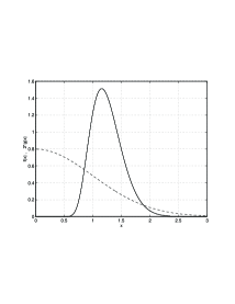
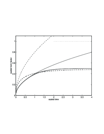
Figure 1: Left plot: The scaled probability distribution of the explored volume for a disordered chain (solid line), compared with a Gaussian distribution that characterizes the diffusion profile (dashed line). Right plot: The scaled form factor for a disordered infinite chain. Solid line - GUE result, Dashed line - GOE result. The thiner curves are obtained by employing the diagonal approximation, while the thicker curves are obtained by employing the BLC approximation scheme. The dotted line illustrates the correct asymptotic behavior.

The average volume which is explored by a POs of length $t$ will be denoted by $\Omega_{e}(t)$. For $d{=}1$ obviously $\Omega_{e}(t)\propto\sqrt{t}$, while for $d{>}2$ the average volume which is explored after time $t$ is $\Omega_{e}(t)\sim t$ to leading order. Specifically, one may write $\Omega_{e}(t)=\ell_{0}^{d_{0}}(t/t_{0})F(t/t_{0})$ where, following [13],

$$F(\tau)=\left\{\matrix{\sqrt{\frac{8}{\pi}}\frac{1}{\tau^{1/2}}&\mbox{for}\ \ d{=}1\cr\pi\frac{1}{\ln(\tau)}&\mbox{for}\ \ d{=}2\cr c+\frac{c^{\prime}}{\tau^{(d{-}2)/2}}&\mbox{for}\ \ 2{<}d{<}4\cr c+\frac{c^{\prime\prime}}{\tau}&\mbox{for}\ \ 4{<}d}\right.$$ (16)

Above $c$ and $c^{\prime}$ and $c^{\prime\prime}$ are constants of order unity (for simple cubic-like structure $c\sim 0.7$). Note that the numerical prefactor $\sqrt{8/\pi}$ for the $d=1$ case in (16) is somewhat larger than the $\sqrt{\pi/2}$ which is implied by (15). This difference is probably due to the fact that (16) is not an exact result if POs are concerned, rather it is an exact result for wandering trajectories. The transient time $t_{0}$ is actually a statistical entity, hence, associated with $\Omega_{e}(t)$ one should consider a dispersion $\Delta\Omega_{e}(t)\approx\ell_{0}^{d_{0}}{\cdot}\sqrt{t/t_{0}}$. Note that in case of Eq.(15), the average explored volume and its dispersion are derived from a one-parameter scaling relation. This is not the case for $1<d$ diffusive system.

It is essential to distinguish the average explored volume $\Omega_{e}(t)$ from the diffusion volume $\Omega_{d}(t)$. The latter is determined by the diffusion law $\Omega_{d}(t)=\ell_{0}^{d_{0}{-}d}({\cal D}_{0}t)^{d/2}$. The diffusion volume $\Omega_{d}$ refers to the instantaneous profile of an evolving distribution. It equals roughly to the total volume of those cells which are occupied by the evolving distribution. Note that $P_{cl}(t)\approx\Omega/\Omega_{d}(t)$.

Given the distribution $f_{t}(\Omega)$, expression (13) can be cast back into the concise form $K(k,t)=C(k,t)K_{D}(t)$ with

$$C(k,t)\ =\ \int_{0}^{\infty}f_{t}(\Omega)d\Omega\ \hat{C}(k\lambda(\Omega,t))\ \ .$$ (17)

The diffusive behavior that corresponds to the diagonal approximation prevails as long as the condition $2\pi<k\lambda(\Omega_{e}(t))$ is satisfied. This condition can be cast into the more suggestive form $t<t_{H}(\Omega_{e}(t))$. The equivalence of latter inequality with the former should be obvious from the discussion of the classical correlation scale in section 4. (There we had taken the reverse route in order to deduce the expression for the classical correlation scale that correspond to a simple ballistic billiard). The concept of running Heisenberg time $t_{H}(\Omega_{e}(t))$ emerges in a natural way from our semiclassical considerations. Originally, this concept has been introduced on the basis of a heuristic guess by Allen. In his paper [2] the concept appears in connection with the tight binding Anderson model where the on site energies are distributed within range $V$ and the hoping probability is $W$. There $g_{0}\sim W/V$. Allen has pointed out that a qualitative agreement with the predictions of scaling theory is recovered if $\xi^{d}$ in (2) is replaced by $\Omega_{e}(t)$ as in our formulation. The condition $t<t_{H}(\Omega_{e}(t))$ for having a diffusive-like behavior can be cast into the form $F(t/t_{0})>1/g_{0}$. It is easily verified that for both $d{=}1$ and $d{=}2$ the results for the breaktime are consistent with (4) and (5). For $d{=}3$ the existence of critical conductance $g_{c}=c^{-1}$ is a natural consequence, but the exponent in (6) is $2/(d{-}2)$ rather than $\nu d$.

Figure 2: The different time regimes for quantal evolution (vertical axis) versus disorder (horizontal axis), for one-two-three dimensional system. The ballistic (B), diffusive (D), critical (C), ergodic (E) and Recurrence (R) regimes are labeled. See further explanations of these diagrams in the text.

Figure 2 illustrates the different time regimes for quantal evolution versus disorder for $d=1,2,3$. These diagrams constitute an improvement [14] over those of [15] and [6]. For ‘zero disorder’ $t_{0}$ may be interpreted as the ballistic time scale that corresponds to the shortest PO. The breaktime is volume limited and determined by the Heisenberg time (1). As the disorder grows larger, two distinct classical time scale emerge, now $t_{0}$ is the ergodic time with respect to one cell, and $t_{erg}$ is the actual time for ergodicity over the whole volume. The latter is determined by the diffusion coefficient as in (14). If the disorder is not too large, the breaktime is still limited by the Heisenberg time. Going to the other extreme limit of very large disorder ($g_{0}<1$) is not very interesting since the particle will be localized within the volume of a single cell. For weaker disorder there is a crossover from a diffusive-like behavior (which is actually anomalous for $d{=}3$) to localization. The crossover time is determined by equations (4-6). In one dimension the crossover from ‘Heisenberg limited’ breaktime to ‘disorder limited’ breaktime happens to coincide with the classical curve for $t_{erg}$. This coincidence does not occur in $d{=}2$ and therefore we have an intermediate regime where the breaktime occurs after ergodization, but is still disorder limited rather than volume limited. In three dimensions we have a qualitatively new regime $g_{c}<g_{0}$ where a purely diffusive (ohmic) behavior (rather than diffusive-like behavior) prevails. The breaktime here is volume limited. Still, the border between the ohmic regime and the so-called ‘critical’ one is non-trivial. Scaling theory predicts that the ohmic behavior is set only after a transient time $t^{**}$ which is given by (6) with $g_{c}{<}g_{0}$. In order to give a semiclassical explanation for $t^{**}$ we should refine somewhat our argumentation. The condition for purely ohmic behavior becomes $t<t_{H}(\Omega_{e}(t){-}\Delta\Omega_{e}(t))$. If $g_{0}$ is close to $g_{c}$ then there will appear a transient time $t<t^{**}$ where the bare diagonal approximation is unsatisfactory. Note however that the critical exponent turns to be by this argumentation $2$ rather than $\nu d$.

6 The BLC approximation scheme

We focus our attention on the actual computation of the form factor $K(\tau)$. Irrespective of any particular assumption it is easily verified that $K(t_{0}){=}t_{H}/g_{0}$, while the asymptotic value $K_{qm}(t){=}t_{H}$ should be obtained for sufficiently long time. The asymptotic behavior reflects the discrete nature of the quantal spectrum. This feature imposes a major restriction on the functional form of $\hat{C}(\kappa)$. Using $\hat{C}_{ballistic}(\kappa)$ (see discussion after (12)) one obtains that for a simple ballistic billiard there is a scaling function such that $K(t)=\Omega\hat{K}_{0}(t/\Omega)$, where $\Omega$ is the total volume. The correct asymptotic behavior is trivially obtained since by construction $\hat{C}_{ballistic}(\kappa)$ gives the correct quantum mechanical result.

For a disordered quasi-1D billiard, in order to determine the form factor, we should substitute (15) into (17). However, also the scaling function $\hat{C}(\kappa)$ should be specified. In order to make further progress towards a quantitative theory let us assume that it is simply equal to $\hat{C}_{ballistic}(\kappa)$. Using this assumption of “ballistic like correlations” (BLC) one obtains that the form factor satisfies the expected scaling property $K(t)=\Omega\hat{K}_{d}(t)$. The latter scaling property, which implies the existence of a characteristic scaling function $\hat{K}_{d}(\tau)$, distinguishes a system with localization. Using the BLC approximation scheme the calculated $\hat{K}_{1}(\tau)$ is

$$\hat{K}_{1}(\tau)\ =\ \frac{1}{\sqrt{2\pi}}\int_{0}^{\infty}dx\ f\left(\frac{x}{\sqrt{\tau}}\right)\ \frac{x}{\tau}\hat{K}_{0}\left(\frac{\tau}{x}\right)\ \ \ \ .$$ (18)

It is plotted in Figure 1. Indeed the breaktime is disorder limited rather than volume limited. However, one observes that the computation yields the asymptotic behavior $K_{qm}(t){=}t_{H}/2$ rather than $K_{qm}(t){=}t_{H}$. This implies that the classical correlations have been overestimated by the BLC approximation scheme.

The BLC approximation scheme can be applied for the analysis of $1<d$ localization. As in the $d{=}1$ case, the correct asymptotic behavior is not obtained. The only way to guarantee a correct asymptotic behavior is to conjecture that $\hat{C}(\kappa)=(\Omega_{d}(t)/\Omega_{e}(t))\hat{C}_{ballistic}(\kappa)$ for $\kappa{<}1$. This required assumption implies that in spite of the net repulsion, the classical spectrum is further characterized by strong clustering. The effective clustering may be interpreted as arising from leaking of POs via ‘transverse’ holes, thus leaving out bundles of POs. Note that the normalization of $p(x)$ does not hold due to the leaking. Therefore $\hat{C}(\kappa)$ is modified in a way that is not completely compatible with its ballistic scaling form.

For completeness we note that in the ‘critical regime’ of $d=3$ localization, it has been suggested [15] to put by hand the information concerning the anomalous sub-diffusive behavior known from scaling theory. One obtains $\mbox{``}P_{c\ell}(t)\mbox{''}\sim({\cal L}/\ell_{0})^{d}{\cdot}(t_{0}/t)$ and hence $K(t)$ is essentially the same as for $d{=}2$ system. The semiclassical justification for this procedure is not clear (see however Ref [16]). We believe that a better strategy would be to find the functional form of $f_{t}(\Omega)$ and $\hat{C}(\kappa)$ and to use (17).

7 Concluding Remarks

We have demonstrated that simple semiclassical considerations are capable of giving an explanation for the existence of a disordered limited breaktime. Qualitatively, the results for the breaktime were in agreement with those of scaling theory of localization. In the last section we have briefly discussed the question whether future quantitative semiclassical theory for localization is feasible. It turns out that the simplest (BLC) approximation scheme overestimates the rigidity of the classical spectrum.

I thank Harel Primack and Uzy Smilansky for interesting discussions. Thomas Dittrich and Shmuel Fishman are acknowledged for their comments. One of the referees is acknowledged for contributing the first paragraph of this paper. This research was supported by the Minerva Center for Nonlinear Physics of Complex systems.

References

- [1] N. Argaman, F.M. Dittes, E. Doron, J.P. Keating, A.Y. Kitaev, M. Sieber and U. Smilansky, Phys. Rev. Lett. 71, 4326 (1993). J.P. Keating in Proceedings of the International School of Physics ”Enrico Fermi”, Course CXIX, Ed. G. Casati, I. Guarneri and U. Smilansky (North Holland 1993).
- [2] P.B. Allen, J. Phys. C 13, L667 (1980).
- [3] M.A. Sepulveda, S. Tomsovic and E.J. Heller, Phys. Rev. Lett. 69, 402 (1992).
- [4] by H.Primack et al. in PRL 76, 1615 (1996)
- [5] M.V. Berry, Proc. R. Soc. London A400, 229 (1985).
- [6] T. Dittrich, Phys. Rep. 271, 267 (1996).
- [7] B.V. Chirikov, F.M. Izrailev and D. Shepelyansky, Sov. Sci. Rev. C 2, 209 (1981).
- [8] R.Scharf and B.Sundaram, PRL 76, 4907 (1996).
- [9] D. Cohen, H. Primack and U. Smilansky, ”Quantal-Classical Duality and the SCTF”, chao-dyn/9708017 (to be published in Annals of Physics).
- [10] E. Abrahams, P.W. Anderson, D.C. Licciardello and T.V. Ramakrishnan, Phys. Rev. Lett 42 673 (1979). For general review see Y. Imry Introduction to Mesoscopic Physics (Oxford Univ. Press 1997).
- [11] M.C. Gutzwiller, Chaos in Classical and Quantum Mechanics (Springer-Verlag, New York, 1990).
- [12] E. Doron, U. Smilansky and T. Dittrich, Physica B179, 1 (1992). N. Argaman, U. Smilansky and Y. Imry, Phys. Rev. B47, 4440 (1993).
- [13] E.W. Montroll and G.H. Weiss, J. Math. Phys. 6, 167 (1965).
- [14] Comparing to [6] the main differences are: The diagram should be distinguished from the diagram since the former should include an intermediate regime; The role of Heisenberg time for should be manifest in the ohmic regime; The localization axis should be appropriately placed.
- [15] A.G. Aronov, V.E. Kravtsov and I.V. Lerner, Phys. Rev. Lett. 74 1174 (1995).
- [16] J.T.Chalker, I.V.Lerner and R.A.Smith, Phys. Rev. Lett. 77, 554 (1996).