Controlling extended systems with spatially filtered, time-delayed feedback

Abstract

We investigate a control technique for spatially extended systems combining spatial filtering with a previously studied form of time-delay feedback. The scheme is naturally suited to real-time control of optical systems. We apply the control scheme to a model of a transversely extended semiconductor laser in which a desirable, coherent traveling wave state exists, but is a member of a nowhere stable family. Our scheme stabilizes this state, and directs the system towards it from realistic, distant and noisy initial conditions. As confirmed by numerical simulation, a linear stability analysis about the controlled state accurately predicts when the scheme is successful, and illustrates some key features of the control including the individual merit of, and interplay between, the spatial and temporal degrees of freedom in the control.

I introduction

Nonlinear dynamical systems often possess periodic orbits that have desirable properties but are unstable. The problem of applying small perturbations to the system in such a way as to produce stable periodic behavior has received much attention recently. [1] This paper addresses the control problem as it arises in a specific context: the stabilization of unstable traveling wave states of spatially extended systems. Though such states have a particularly simple structure, the control problem is nontrivial.

The general method introduced below may be applicable to a wide variety of physical systems, but an entirely general analysis of it is beyond the scope of this work. We have chosen to investigate in detail its application to two sets of model equations describing the dynamics of wide aperture semiconductor lasers. Our results demonstrate that unstable traveling wave states can be effectively controlled in these systems and therefore have implications both for the general theory of control of spatially extended systems and for the design of semiconductor lasers.

For the purposes of this paper, controlling a system means providing feedback that locks the system to one member of a possibly infinite family of unstable periodic orbits present in that system, thereby choosing a desired state from a large variety of possibilities. The technological goal is to produce a desirable behavior in a system by applying carefully chosen feedback that directs the system to the goal state and keeps it there. For many applications, it is desirable to design the feedback such that the magnitude of the control signal decreases as the system approaches the desired state, and, in the absence of noise, vanishes when the controlled behavior is a dynamical state of the uncontrolled system. It is also worthwhile to consider “controlling” a state which is only approximately a true orbit of the system. An important example is the situation where a stress is applied to a large but finite transverse portion of a system. Useful results for the dynamics of the active region may still be obtained by using feedback designed for the traveling wave solution of the infinite, idealized system. In this case one might expect the feedback to become small, but not completely vanish.

For a system with an accessible dynamical field $A(x,t)$, our control signal $\epsilon_{A}({\bf x},t)$ is derived from an infinite sum of signals delayed in time by integer multiples of the period of the state that is to be stabilized:

$$\epsilon_{A}({\bf x},t)=$$ (2)

$$\gamma\left[A({\bf x},t)-(1-R)\sum^{\infty}_{n=1}R^{n-1}{\tilde{A}_{n}}({\bf x},t-n\tau)\right],$$

where $\gamma$ is the gain of the feedback, $\tau$ is the period of the target state, and $0\leq R<1$ determines the relative weight given to states farther in the past. The field ${\tilde{A}_{n}(x,t)}={\cal F}^{-1}[f^{2n}(k-k_{c}){\cal F}[A(x,t)]]$ is the spatially filtered version of $A$. Here $f()$ is a filtering function applied in Fourier space and ${\cal F}[A]$ is the spatial Fourier transform of $A$. The precise manner in which the spatial filtering is included may vary; we have made a choice that corresponds directly to an experimental arrangement described below. We take $f(q)$ to be peaked around zero so that contributions to $A$ from wave numbers other than the desired wave number, $k_{c}$, are suppressed in ${\tilde{A}}$. We also take $f(0)=1$ so that the feedback term vanishes identically when the system is in a pure state of wave number $k_{c}$ that is an unstable orbit of the uncontrolled system. Eq. 2 represents the enhancement of time-delay feedback of the form analyzed in Ref. [3] with spatial filtering of the type introduced in Ref. [2].

Control based on Eq. 2 is especially well-suited to spatially extended states with a structure dominated by one Fourier mode. Feedback occurs whenever there are components in the system due to undesired wave numbers or undesired frequencies. The temporal feedback is important both because practical implementations of the spatially filtered feedback necessarily involve time delays and because spatially filtered feedback alone is sometimes not sufficient to stabilize the desired state.

We emphasize that the control scheme investigated here is a plausible candidate for implementation in experimental systems. As in Ref. [3], a form of time-delay feedback is used which includes previous comparisons made between the state and a time-delayed version in a way that is easy to implement because the feedback signal can be generated recursively. [4] This is a generalization of a low-dimensional control technique known as extended time-delay autosychronization, [5] which is in turn a generalization of a scheme introduced by Pyragas [6] and has been demonstrated to work in low-dimensional electronic systems. [5]

Optical systems are of particular interest with respect to control both because they offer excellent laboratories for testing theoretical ideas and because important technological problems associated with them may be solved through control techniques. Wide aperture semiconductor lasers, with their compact size and very large gain, are ideal candidates for high brightness coherent steerable laser sources (spatially and temporally coherent). However, the pronounced asymmetry in their gain and refractive index spectra leads to a very strong nonlinear amplitude-phase coupling in the laser field. Consequently, wide aperture semiconductor lasers display uncontrolled dynamic intensity filamentation (random beam steering) even immediately beyond lasing threshold. This behavior persists and becomes even more complicated at higher current pumping levels. Moreover the timescales involved in the laser dynamics lie in the nanosecond to picosecond regime, ruling out any algorithm which requires indirect intervention in order to establish control. Time delay feedback with real-time filtering in space and time is a natural candidate for all-optical control of these systems.

To illustrate the power of spatially filtered, time delay feedback, we analyze the important example of the laser Swift-Hohenberg equations which approximately describe the dynamics of the optical field of a wide aperture semiconductor laser with one transverse dimension. Results of linear stability analyses are used to guide the choice of control parameters for numerical simulations, which reveal that the controlled state may be attained even when the initial conditions are far from the linear regime. Also, because semiconductor edge-emitting lasers typically run on multiple longitudinal modes, we study the case of a two-longitudinal mode laser Swift-Hohenberg model. We find that the presence of a second mode introduces new features relevant to the control scheme, but that control is still possible.

Our primary motivation for studying this particular system is that the feedback signal of interest can be produced using a Fabry-Perot interferometer containing a spatial filter. The time delay in the feedback scheme corresponds to the round trip transit time in the interferometer. The spatial filtering can be accomplished by a focusing lens, whose focal plane contains the far-field fluctuating output of the laser. Placing a suitable aperture in the focal plane of the lens acts as a narrow band spatial filter. One example of a suitable arrangement for generating the desired feedback is shown in Fig. 1. Our results therefore suggest a feasible approach to the suppression of unwanted spatiotemporal fluctuations in real laser systems.

One of the main results of the present paper is that the addition of spatial filtering to time-delay control (using ${\tilde{A}_{n}}$ rather than $A_{n}$ in Eqn. 2) produces a highly robust control scheme. In the context of the laser equations discussed below, linear stability analysis of the infinite system shows that in general both the spatial filtering and the time delay are important components of the scheme. For the models we study, numerical results also show that when a state is stable with feedback it is also highly attracting, so that linear stability analysis is predictive even far from the linear regime. Simulations of the model equations show that the feedback is able to direct the system towards the desired state from a distant initial condition, and that spatial filtering is the dominant mechanism responsible for this behavior.

Before proceeding to the detailed analysis of our scheme, we mention some related investigations. First, results of numerical simulations of the application of our scheme with $R=0$ to the control of traveling wave solutions in the single longitudinal mode semiconductor laser Swift-Hohenberg equations (discussed below), have been reported elsewhere. [2] There, the spatial filtering was shown to be extremely robust, rapidly suppressing the broadband noisy spatial spectrum of the free running unstable laser, in favor of the filtered transverse traveling wave mode. The subsequent evolution towards a controlled state was observed to depend sensitively on whether the system is infinitely extended (idealized) or pumped over a finite transverse cross-section. In the former case, the system evolves to a pure nonlinear traveling wave mode of the isolated laser system, although at higher stress the system typically spent time in a metastable dynamical state before reaching the desired traveling wave. For finite transverse pumping, the system evolves to a mixed traveling wave solution of the joint laser-feedback system and remains there. In this latter case, a finite amount of energy remains in the feedback loop.

Second, Lu et al. [7] considered feedback constructed by combining comparisons of the current state of the system both to a version delayed by the temporal period of the target state and to versions shifted by the spatial period of the target state. Numerical integration showed that the control can direct the system towards, and stabilize, a pattern in a transversely extended laser model, but the method does not appear to be a good candidate for all-optical implementation.

Finally, Battogtokh et al. [8] considered the effect of feeding back a time-delayed signal constructed from the global average of a dynamical field, showing that stable uniform oscillatory states of the system with feedback exist for some choices of the delay time. In the scheme they analyze, the control signal does not represent a small perturbation and the delay time is not tuned to the period of the desired orbit.

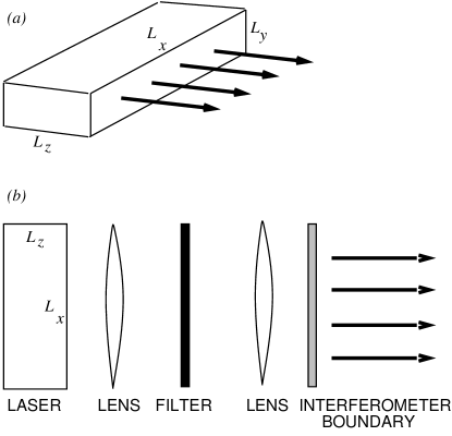
FIG. 1.: (a) Geometry of a wide aperture laser. $L_{y}$ is assumed to be sufficiently small that only one mode dominates in the $y$-direction. The large width $L_{x}$ gives rise to many transverse modes. The linear stability analysis in this paper is valid for arbitrarily large $L_{x}$. The size of $L_{z}$ determines the number of longitudinal modes that are relevant for the dynamics. (b) One possible schematic implementation of the feedback mechanism studied in this paper. The feedback signal is the field reflected from the front of the laser cavity in the presence of an additional reflecting interface (labeled “Interferometer Boundary”). The spatial filtering is performed by the two lenses with a filter placed at the focal plane of each.

II Single longitudinal mode laser swift-hohenberg equations

We now treat the specific example of a recently derived model of the transversely extended semiconductor laser, the semiconductor laser Swift-Hohenberg equations, [9] extending the results of Ref. [2]. The model assumes the cavity geometry shown in Fig. 1(a) with $L_{y}$ and $L_{z}$ both small enough that the dynamics is dominated by a single mode in the $y$ and $z$ directions, but $L_{x}$ large. Denoting the $x$-dependent envelope of the electric field by the complex field $\psi$ and the carrier density by the real field $n$, the equations are

$$(\sigma+1)\partial_{t}\psi = \sigma(r-1)\psi+ia\nabla^{2}\psi-i\sigma\Omega\psi$$ (5)

$$-\frac{\sigma}{(1+\sigma)^{2}}(\Omega+a\nabla^{2})^{2}\psi$$

$$-\sigma(1+i\alpha)n\psi+\epsilon_{\psi}$$

$$\partial_{t}n = -bn+|\psi|^{2}$$ (6)

where $\sigma$ and $b$ are the decay rates of the electric field and population inversion respectively, normalized to the decay rate of the polarization, $r$ is the scaled pump rate, $a$ is a scaled diffusion constant, $\Omega$ is the detuning between the atomic and carrier frequencies, and $\alpha<0$ is a nonlinear amplitude-phase coupling. (All the coefficients in the equation are real.)

The model is similar to the laser Swift-Hohenberg equations [10] for two-level lasers. The key difference in the semiconductor equations is the explicit inclusion of the $\alpha$ term which derives from the strong assymmetry in the semiconductor optical gain and refractive index spectra [11, 12]. Other terms arising in the semiconductor version due to spectral hole burning in the carrier distributions do not influence the results discussed here.

With control turned off ($\epsilon_{\psi}=0$), Eqns. (5) and (6) have traveling wave solutions that are always unstable [10]:

$$\psi_{k}(x,t) = \rho\exp i(kx-\omega t+\phi),$$ (7)

$$n_{k} = \rho^{2}/b,$$ (8)

where $\phi$ is an arbitrary phase that will henceforth be assumed to be zero,

$$\ \rho^{2} = b\left[r-1-\left(\frac{\Omega-ak^{2}}{1+\sigma}\right)^{2}\right],$$ (9)

$$\omega = \frac{\sigma\Omega+ak^{2}+\alpha\sigma\rho^{2}/b}{1+\sigma}.$$ (10)

Note that $\rho$ is real and that the traveling wave solution ceases to exist when the right-hand side of Eqn. (9) is negative.

Eqn. (5) for the envelope of the electric field contains a time-delay and spatial filtering control term of the form of Eqn. (2), with the time delay $\tau$ set to $2\pi/\omega$, the period of the desired traveling wave state. The insertion of the feedback as simply an additive term in this equation is an approximation of the real effect of the feedback, which actually consists of an electric field applied at the front face of the laser cavity due to reflections from the elements shown in Fig. 1(b). The gain $\gamma$ should be thought of as a phenomenological parameter that characterizes the effect of this boundary term on the longitudinal mode in question. The optimal choice of the filter function $f$ is not immediately clear. For now we take $f(q)$ to be a gaussian of width $\Gamma$; i.e., $f(q)=\exp[-q^{2}/\Gamma^{2}]$. As explained below, the results are not sensitive to the precise choice of $\Gamma$. The case of a square filter function is also discussed briefly below.

To perform the linear stability analysis we write $\psi(x,t)=[1+B(x,t)]\psi_{k}$ and $n(x,t)=[1+C(x,t)]n_{k}$, and arrive at the following linearized equations in the vicinity of a traveling wave solution:

$$(\sigma+1)\partial_{t}B = -(2ak+4iak{\tilde{\sigma}}\Omega-4ia^{2}{\tilde{\sigma}}k^{3})\nabla B$$ (14)

$$+(ia-2a{\tilde{\sigma}}\Omega+6{\tilde{\sigma}}a^{2}k^{2})\nabla^{2}B$$

$$-4i{\tilde{\sigma}}a^{2}k\nabla^{3}B-{\tilde{\sigma}}a^{2}\nabla^{4}B$$

$$-(1+i\alpha)\frac{R^{2}}{b}\sigma C+\epsilon_{B}$$

$$\partial_{t}C = b(B+B^{*}-C),$$ (15)

where ${\tilde{\sigma}}\equiv\sigma/(1+\sigma)^{2}$.

FIG. 2.: (a) Growth rates of perturbations of an uncontrolled ($\gamma=0$) traveling wave solution of Eqns. (8,9) with $k=5$ and $r=1.5$. and parameter values $\sigma=.1$, $\Omega=.001$, $a=.01$, $b=.01$, and $\alpha=-5$. For each $q$, ${\bf Re[\lambda]}>0$ implies exponential growth of the perturbation. (b) Stable region in the $q,\gamma$ plane of the same traveling wave with control. The solid line is the stability boundary for $R=0$, $\tau=2\pi/\omega$, and $\Gamma=.25$. Note that all modes are stable for $\gamma<-0.1$. The dashed line (see inset) corresponds to the (unphysical) case of $\tau=0$, $R=0$.

Following Ref. [3], we obtain a linear system of ordinary differential equations for the Fourier modes of the perturbation. Letting ${\bf\xi}=(B_{q},B^{*}_{q},C_{q})$, the 3D vector of Fourier amplitudes at wave number $q$, the equations can be written in the general form

$$\frac{d}{dt}{\bf\xi}={\bf J}\cdot{\bf\xi}+{\bf M}\cdot\epsilon_{\bf\xi},$$ (16)

where $\epsilon$ is given by the expression in Eqn. (2), ${\bf J}$ is obtained from the coefficients of Eqns. (14) and (15), and ${\bf M}$ is determined by which variables form the control signal and how the control signal enters the equations. In the present case,

$${\bf M}=\left(\begin{array}[]{ccc}1&0&0\\ 0&1&0\\ 0&0&0\end{array}\right).$$ (17)

The factor by which a given eigenmode of the perturbation grows during one period of the evolution of the controlled system is called a Floquet multiplier. The time delay in the control term requires that the initial conditions for the evolution must specify the behavior over an entire continuous time interval of one period, so each spatial Fourier mode has an infinite number of eigenmodes and Floquet multipliers, $\mu_{j}$. Letting ${\bf\xi}^{(j)}$ represent the $j^{th}$ eigenmode, we have, by definition,

$${\bf\xi}^{(j)}(t+\tau)=\mu_{j}{\bf\xi}^{(j)}(t).$$ (18)

The set of Floquet multipliers for a perturbation with wave number $q$ determine that perturbation’s linear stability; if one or more multiplier has $|\mu_{j}|>1$, the perturbation is unstable.

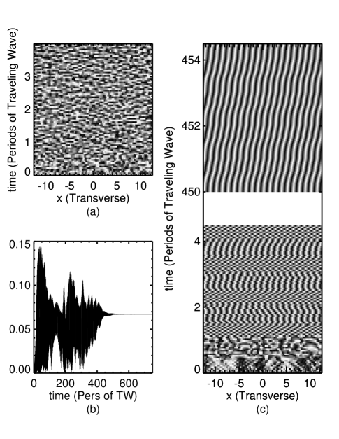
FIG. 3.: Evolution of the single mode system with $a,b,\Omega,\sigma,\alpha,r,k$ as in Fig. 2a. , and $\gamma=.2$. (a) A spacetime plot of the phase of the field $\psi$ in the uncontrolled system showing chaotic fluctuations. (b) The growth of the magnitude of the desired mode as a function of time. (c) A spacetime plot of the phase of $\psi$ in the controlled system for the same run as shown in (b). The lower region shows the dynamics when the system is first turned on. After a short period during which fluctuations grow rapidly, the feedback suppresses all wave numbers other than the desired one. After a transient time of approximately 500 periods of the desired orbit, the system settles into the traveling wave state. The upper portion shows the system as as it approaches the desired state, which would appear as straight bands on this plot.

Dropping the subscript $j$ and evaluating the geometric sum in $\epsilon$, Eqn. (16) may be written

$$\frac{d}{dt}{\bf\xi}={\bf J}\cdot{\bf\xi}+\gamma\left(\frac{1-f^{2}(q)\mu^{-1}}{1-Rf^{2}(q)\mu^{-1}}\right){\bf M}\cdot{\bf\xi}.$$ (19)

The values of the Floquet multipliers are determined by requiring consistency between this equation and the defining relation of Eqn. (18). We obtain the following characteristic equation for this modified eigenvalue problem:

$$g(\mu^{-1})=\left|\mu^{-1}e^{\tau\left[{\bf J}+\gamma\left(\frac{1-f^{2}(q)\mu^{-1}}{1-Rf^{2}(q)\mu^{-1}}\right){\bf M}\right]}-1\!\!1\right|=0,$$ (20)

where the exponential represents the operator that advances the linear system by one period $\tau$. As discussed in Refs. [13, 3], one can perform a numerical winding number calculation of $g(\mu^{-1})$ around the unit circle to obtain the number of roots satisfying $|\mu^{-1}|<1$. Since there are no poles in the unit disk, the system is linearly stable if and only if this winding number vanishes.

Results from the linear stability analysis predict that our control technique successfully stabilizes all traveling wave solutions in the single longitudinal mode model. We present detailed results for a single traveling wave solution, for $k=5$ and $r=1.5$, which is typical of all traveling waves we have studied. (Values of the other parameters are given in the caption.)

Fig. 2a shows the growth rates of the modes of the uncontrolled system, which are obtained by finding the eigenvalues of ${\bf J}$ in Eqn. 16. There is one unstable mode for perturbation wave numbers between zero and $\sim 12$. With control, using $R=0$, we find that the traveling wave state is stable for $\gamma$ sufficiently negative. The solid line in Fig. 2b indicates the boundary between which perturbation wave numbers are stable or unstable at a given $\gamma$. The controlled traveling wave is stable at values of $\gamma$ for which all wave numbers are stable, i.e., where the shaded region contains an entire horizontal line. For all traveling waves in this model, there is a minimum $|\gamma|$ for which the state is stable. In the case shown in Fig. 2b, this occurs at $\gamma\sim-.1$. In this model, there is no lower boundary to the stable region for traveling waves.

We find for this system that spatial filtering alone would be sufficient to stabilize the traveling wave. The stability boundary obtained with $\tau=0$ and $R=0$, the dashed line in Fig. 2b, is nearly identical to the one with $\tau=2\pi/\omega$ at large $q$, but the time delay clearly has a significant effect at $q$ near zero. It is also important to note that implementation of a spatial filter with no time delay is not possible in fast optical systems. The result that the introduction of a time delay of one period does not destroy the stability in the case of the gaussian filter is therefore significant.

In general, a given wave number perturbation can be stabilized either by the time delay feedback with no spatial filtering or by the spatial filtering with no time delay. In each case, however, there may be small bands of wave numbers for which one or the other method fails. A given spatial filter fails near $q=0$ if there exist perturbations which are sufficiently unstable (or if $f(q)$ is sufficiently close to unity). For $q$’s at which $f(q)=1$, as occurs for a finite band in the step function case, the spatial filtering has no effect on the stability. The time delay feedback alone fails for wave numbers whose frequency of oscillation is sufficiently close to an integer multiple of the frequency of the desired traveling wave. Combining the spatial filter and the time delay renders the system stable at all $q$.

The time delay is a crucial component for stability in the two mode system discussed below. In the single mode system, it may also play an important role if $f(q)$ is chosen to be a step function rather than a gaussian.

The predictions of several stability diagrams similar to Fig. 2b have been checked in detail by numerical simulation. The numerics show that the traveling wave states are stabilized with values of $\gamma$ predicted by the linear analysis, and that instabilities occur at the wave number predicted when $|\gamma|$ is too small.

An important question is whether the linear stability analysis is predictive of the behavior of the system even for initial conditions that are not in the linear regime. Numerical integration of the model equations show that the spatially filtered feedback is particularly effective in directing the system to the desired state. As illustrated in Fig. 3, for parameters corresponding to a linearly stable controlled state, the system is attracted to the desired state from a typical initial condition. Though it is difficult to display the full behavior during the long transient, an investigation of the details reveals that, beginning from low amplitude noise of the type that would be expected when the laser is first turned on, the system, depending on the parameter regime, may pass through several nearly stable states with the desired wave number, but the incorrect frequency, before finally settling on the one with the desired frequency. Preliminary investigations of systems with time delay feedback alone indicate that more complicated behavior occurs beyond the linear regime.

III Two longitudinal mode laser swift-hohenberg equations

Semiconductor lasers of practical interest generally operate in regimes where many longitudinal modes may be active. To begin to understand the possible effects of multiple longitudinal modes, we study a two mode model. This model is a straightforward generalization of the two level, one mode model derived in Ref. [10] to the situation in which two longitudinal modes, with mode separation $2\Delta$, dominate the dynamics. [14] With the addition of the semiconductor $\alpha$ term discussed above, this model reads,

$$(\sigma+1)\partial_{t}\psi_{1} = \sigma(r-1)\psi_{1}+ia\nabla^{2}\psi_{1}+i\Delta\psi_{1}-i\sigma\Omega\psi_{1}$$ (23)

$$-\frac{\sigma}{(1+\sigma)^{2}}(\Omega+\Delta+a\nabla^{2})^{2}\psi_{1}$$

$$-\sigma(1+i\alpha)n\psi_{1}-\sigma(1+i\alpha)\eta\psi_{2}+\epsilon_{\psi}$$

$$(\sigma+1)\partial_{t}\psi_{2} = \sigma(r-1)\psi_{2}+ia\nabla^{2}\psi_{2}-i\Delta\psi_{2}-i\sigma\Omega\psi_{2}$$ (26)

$$-\frac{\sigma}{(1+\sigma)^{2}}(\Omega-\Delta+a\nabla^{2})^{2}\psi_{2}$$

$$-\sigma(1+i\alpha)n\psi_{2}-\sigma(1+i\alpha)\eta^{*}\psi_{1}+\epsilon_{\psi}$$

$$\partial_{t}n = -bn+|\psi_{1}|^{2}+|\psi_{2}|^{2}$$ (27)

$$\partial_{t}\eta = -b\eta+\psi_{1}\psi_{2}^{*}.$$ (28)

Note that the same control term $\epsilon_{\psi}\equiv\epsilon_{\psi_{1}}+\epsilon_{\psi_{2}}$ appears in the both $\psi_{1}$ and $\psi_{2}$ equations with equal magnitude. This simple way to model the effect of the reinjection of the reflected field into the laser cavity is used here for convenience. The present model is intended only to display the new qualitative features that arise when more than one mode is relevant.

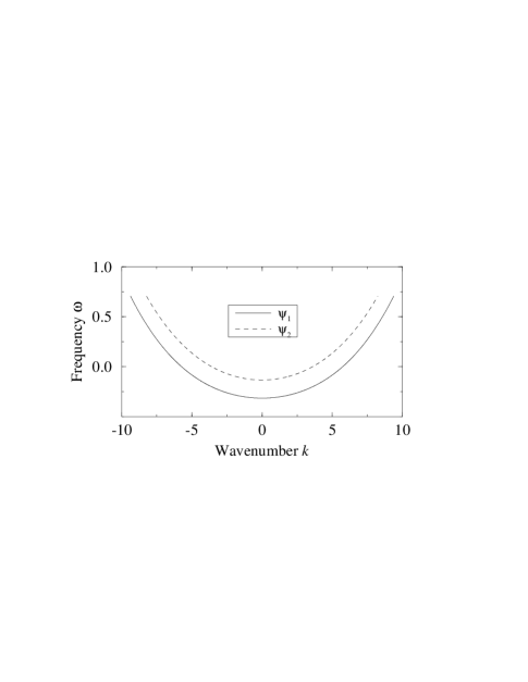
FIG. 4.: Dispersion curves for (unstable) traveling wave solutions in the two mode model. The solid (dashed) line represents solutions in which only the favored (unfavored) mode is excited. The parameters are $\delta=.05$, $\sigma=.1$, $\Omega=.001$, $a=.01$, $b=.01$, and $\alpha=-5$.

We are interested in the solution in which one longitudinal mode supports a traveling wave and the other is inactive:

$$\psi_{1} = \psi_{k}\equiv\rho\exp{i(kx-wt)},$$ (29)

$$n = n_{k}\equiv\rho^{2}/b,$$ (30)

$$\psi_{2} = 0,$$ (31)

$$\eta = 0,$$ (32)

where

$$\rho^{2} = b\left[r-1-\left(\frac{\Omega+\Delta-ak^{2}}{1+\sigma}\right)^{2}\right]$$ (33)

$$\omega = \frac{\sigma\Omega+ak^{2}-\Delta+\alpha\sigma\rho^{2}/b}{1+\sigma}.$$ (34)

The complementary solution is obtained by interchanging the subscripts of the fields and taking $\Delta\rightarrow-\Delta$ in the expresions for $\rho$ and $\omega$. Taking $\psi_{1}=(1+B)\psi_{k}$, $\psi_{2}=D\psi_{k}$, $n=(1+C)n_{k}$, and $\eta=E$, we obtain the following linear equations for the small fields $B,D,C,E$,

$$(\sigma+1)\partial_{t}B = -(2ak+4iak{\tilde{\sigma}}\Omega-4ia^{2}{\tilde{\sigma}}k^{3})\nabla B$$ (36)

$$+(ia-2a{\tilde{\sigma}}\Omega+6{\tilde{\sigma}}a^{2}k^{2})\nabla^{2}B$$

$$(\sigma+1)\partial_{t}D = \left[ia\nabla^{2}-2ik-{\tilde{\sigma}}(\Omega-\Delta+a\nabla^{2})^{2}\right.$$ (39)

$$\left.+iak^{2}+{\tilde{\sigma}}(\Omega+\Delta-ak^{2})^{2}\right]D$$

$$-\sigma(1+i\alpha)E^{*}$$

$$\partial_{t}C = b(B+B^{*}-C)$$ (40)

$$\partial_{t}E = -2bE+\rho^{2}D^{*}$$ (41)

FIG. 5.: (a) Real parts of the eigenvalues of an uncontrolled ($\gamma=0$) solution in which $\psi_{2}$ is a traveling wave with $k=8$ and $r=1.5$, and $\psi_{1}$ is zero everywhere. Parameters are the same as in Fig. 4. (b) Stable region of the same solution with control with parameters $R=.5$, $\tau=2\pi/\omega$, and $\Gamma=.25$. The traveling wave is stable at all $q$ for $-0.13<\gamma<-0.05$.

Fourier transforming, we again obtain a general expression for the behavior of small differences of a perturbation wave number from the controlled state. Letting $q_{x}$ be the wave number in the transverse direction and ${\bf\xi}=(B,B^{*},D,D^{*},C,E,E^{*})$, we have

$$\frac{d}{dt}{\bf\xi}={\bf J}\cdot{\bf\xi}+{\bf M}\cdot\epsilon_{\bf\xi},$$ (42)

where here ${\bf J}$ is the matrix of coefficients obtained directly from Eqns. (36-41) and

$${\bf M}=\left(\begin{array}[]{ccccccc}1&0&1&0&0&0&0\\ 0&1&0&1&0&0&0\\ 1&0&1&0&0&0&0\\ 0&1&0&1&0&0&0\\ 0&0&0&0&0&0&0\\ 0&0&0&0&0&0&0\\ 0&0&0&0&0&0&0\\ \end{array}\right).$$ (43)

As in the case of the single longitudinal mode laser, a condition of the form of Eqn. 20 defines the Floquet multipliers of the system.

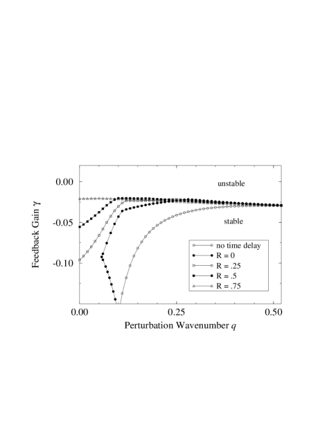
FIG. 6.: A detail from the left edge of the upper boundary of the domain of control in Fig. 5(b) shows the effect of varying $R$. In the case of $R=0$, as with no time delay, the traveling wave solution cannot be controlled due to instabilities at small $q$. Larger values of $R$ do yield stable solutions for sufficiently negative $\gamma$.

We now describe the results of the linear stability analysis of the two mode model. As in the single mode model, each mode is always unstable to transverse fluctuations, but in the two mode model it is possible for one mode to be unstable to the growth of the other as well. A straightforward stability analysis of the uncontrolled equations shows that for all parameter choices both $\psi_{1}$ or $\psi_{2}$ are marginally stable against transverse fluctuations at $q_{x}=0$, but only one of the modes is always stable against growth of the other mode. Which mode is which depends upon the choice of the mode separation, the desired wave number, and other parameters in the model. We will refer to a mode that is stable (unstable) against growth of other longitudinal modes at $q_{x}=0$ as “favored” (“unfavored”).

The dispersion curves for transverse waves in the two modes have nearly the same functional form, but are displaced relative to each other approximately by the mode spacing, $2\Delta$. (See, for example, Fig. 4.) By choosing the wave number for the spatial filter, one selects one traveling wave state from each of the two dispersion curves. Because the frequencies of these two states are different, one can choose the time delay so as to suppress fluctuations at the frequency of the undesired mode. Thus it is plausible to suppose that the combination of the time delay and the spatial filter capable of stabilizing either of the two longitudinal modes. We will focus on the stabilization of an unfavored mode, both because it would appear to be the more difficult case and because it may be a better representation of the situation that arises in multimode systems.

Fig. 5 illustrates the stabilization of the unfavored mode ($\psi_{1}$) with the parameters listed in the caption. Fig. 5a, shows the stability curves for the uncontrolled system, clearly indicating the instability at $q=0$ that makes this case qualitatively different from the single mode case discussed above. The spatial filter component in our control scheme is insensitive to instabilities at or near $q=0$ because the filter must pass components of both $\psi_{1}$ and $\psi_{2}$ with this wave number. The width of the function $f(q)$ used for the spatial filter will determine the range of $q$ which are passed. As a result of the ineffectiveness of the spatial filter over this range of perturbation wave number, the temporal component of the control scheme must be relied on to stabilize these perturbations.

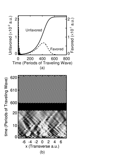
FIG. 7.: Evolution of two mode system with $a,b,\Omega,r,\sigma,\alpha,$ as in Fig. 4. with $\Delta=0.1$, $r=1.5$, $k=8$, $R=0.5$, and $\gamma=.1$. (a) A spacetime plot of the phase of $\psi$ in the controlled system. The lower region shows the dynamics when the system is first turned on. After a transient time of approximately 200 periods of the desired orbit, the system settles into the traveling wave state. (b) The magnitude of the favored mode (dashed line) and unfavored mode (solid line) as a function of time for the same run as shown in (b). Note the expanded scale at the right for the favored mode.

The stability diagrams of Fig. 5b and Fig. 6 demonstrates that the time-delay control is effective in controlling the range of perturbation wave numbers that are not stabilized by the spatial filter. Fig. 5b shows that with both time-delay control (here with $R=0.5$) and the spatial filter (with $\Gamma=0.25$) there is a range of $\gamma$ that stabilizes the traveling wave solution. Fig. 6 shows that when time-delay control is not present, and also when $R$ is too small, there is no range of $\gamma$ that stabilizes the traveling wave solution at all wavenumbers.

A new feature that appears in the two mode model, and is shown in Fig. 5b, is the lower boundary of the stable domain, whose origin lies in the off-diagonal elements of ${\bf M}$. When the system is not exactly on the desired orbit, there is a finite amount of feedback generated. Because the desired mode has a much larger average magnitude than the other mode, the feedback signal is dominated by effects from the desired mode. This feedback is necessary to control the desired mode, but it also affects the other mode. When the magnitude of this feedback becomes too large, as it must when $|\gamma|$ is increased, these unwanted perturbations to the undesired mode cause the state to go unstable.

The position of the lower boundary of the domain of control (Fig. 5b) is important because it determines the range of gain that can be used to obtain control. If that range is very small, it may be difficult to find an appropriate $\gamma$ in an experiment. Even worse, if the lower boundary becomes so high that part of it reaches the lowest point of the upper boundary, there is no $\gamma$ which can control the system. We find that the position of the lower boundary is affected by several parameters. The lower boundary is raised when the pump rate $r$ is raised and when the wave number $k$ is lowered. The mode separation, $\Delta$, also plays an important role in the location of the lower boundary. For larger $\Delta$, the lower boundary is pushed down. In a system in which $\gamma$ is the only adjustable parameter ($r$, $\Delta$, and $R$ fixed), we find that traveling waves with wavenumbers in a finite continuous band can be stabilized. The high-$k$ boundary of the band is determined by the condition that traveling waves exist (that $\rho$ must be real), and the low-$k$ boundary is the point at which there ceases to be a $\gamma$ that can control perturbations at all wave numbers.

As in the single mode model, numerical simulations confirm the predictions of the linear analysis and show that the traveling wave state can be obtained starting from a distant initial condition. Fig. 7 shows the emergence of the desired traveling wave from a low amplitude, noisy initial condition. After an initial transient, the system clearly settles into the desired pure traveling wave.

We have also observed the behavior of the system when $R$ is chosen too small. Although the only unstable modes in this case are very close to $q=0$, we find that their growth completely destroys the traveling wave. The system does not merely develop long wavelength modulations of the desired wave. We therefore conclude that both the temporal and spatial aspects of the feedback signal we have analyzed play essential roles in the success of the scheme.

IV Conclusions

Our study of the dynamics of laser Swift-Hohenberg equations with time-delayed, spatially filtered feedback strongly suggests that stable lasing at a single transverse wave number in wide aperture lasers is possible. A future publication will report on studies of a more realistic model of field and carrier dynamics in a semiconductor system of the type shown in Fig. 1, where preliminary results are encouraging. Though there are several nontrivial experimental issues associated with the fabrication of such a device, we believe that this is a promising direction for research and development.

We have presented a theoretical approach to the analysis of this sort of feedback that appears to capture the relevant features of the dynamics. The linear stability analysis presented here is a straightforward extension of some of previous work on stabilizing traveling waves in the complex Ginzburg-Landau equation. In the present case, however, the desired state seems to be a global attractor, which gives us considerably more confidence in its potential for practical implementation.

Finally, we would like to emphasize that the general method of applying time-delay feedback combined with spatial filtering is a powerful technique that might be adapted to many other types of physical systems. Its primary advantage is that the desired traveling wave state need not be available in some external form for construction of the feedback signal. It is particularly suitable for optical systems, however, where the necessary manipulations of the signal can be performed with standard optical elements.

We thank Dan Gauthier and Rob Indik for helpful conversations. MEB gratefully acknowledges the hospitality of the Arizona Center for Mathematical Sciences. JVM and DH were supported by AFOSR-94-1-0144DEF and AFOSR-94-1-0463. JESS and MEB were supported by NSF Grant DMR-94-12416.

REFERENCES

- [1] E. Ott and M. Spano, Phys. Today 48, No. 5, 34 (1995) and references therein.
- [2] D. Hochheiser, J. Lega, and J. V. Moloney, preprint.
- [3] M. E. Bleich and J. E. S. Socolar, Phys. Rev. E 57 R16 (1996).
- [4] For a discussion of the experimental implementation of including past comparisons recursively in the context of an electrical circuit, see Ref. [5].
- [5] D. J. Gauthier, D. W. Sukow, H. M. Concannon, and J. E. S. Socolar, Phys. Rev. E 50, 2343 (1994); J. E. S. Socolar, D. W. Sukow, and D. J. Gauthier, Phys. Rev. E 50, 3245 (1994).
- [6] K. Pyragas, Phys. Lett. A 170, 421 (1992); K. Pyragas and A. Tamas̆evic̆ius, Phys. Lett. A 180, 99 (1993); A. Kittel, J. Parisi, and K. Pyragas, Phys. Lett. A 198, 433 (1995).
- [7] W. Lu, D. Yu, and R. G. Harrison, Phys. Rev. Lett. 76, 3316 (1996).
- [8] D. Battogtokh and A. Mikhailov, Physica D 90, 84 (1996).
- [9] C. Bowman et al., preprint.
- [10] J. Lega, J. V. Moloney, and A. C. Newell, Phys. Rev. Lett. 73, 2978 (1994) and Physica D 83, 478 (1995). In contrast to the semiconductor model, the regular laser Swift-Hohenberg equations the traveling waves are stable within some region in parameter space known as the Busse balloon.
- [11] C.H. Henry, Theory of the linewidth of semiconductor lasers, IEEE J. Quant. Electron., Vol. QE-18, 259 (1982).
- [12] W. W. Chow, S. W. Koch, and M. Sargent, Semiconductor Laser Physics, Springer, Heidelberg, Berlin, 1994
- [13] M. E. Bleich and J. E. S. Socolar, Phys. Lett. A (1996).
- [14] The small mode separation, is assumed to have a magnitude which is first order in the expansion of Ref. [10].