Synchronization of Spatiotemporal Chaos:
The regime of coupled Spatiotemporal Intermittency

Abstract

Synchronization of spatiotemporally chaotic extended systems is considered in the context of coupled one-dimensional Complex Ginzburg-Landau equations (CGLE). A regime of coupled spatiotemporal intermittency (STI) is identified and described in terms of the space-time synchronized chaotic motion of localized structures. A quantitative measure of synchronization as a function of coupling parameter is given through distribution functions and information measures. The coupled STI regime is shown to dissapear into regular dynamics for situations of strong coupling, hence a description in terms of a single CGLE is not appropiate.

Two issues of high current interest in the general field of nonlinear dynamics are the quantitative characterization of different regimes of spatiotemporal complex dynamics in extended systems [4] and the synchronization of chaotic oscillators [5]. The characterization of low dimensional chaos is now a mature subject with well established techniques, including techniques of chaos control. In this context, the demonstration that the familiar phenomenon of synchronization of two regular oscillators [6] by a weak coupling can also be displayed by chaotic oscillators is an important new idea. This conceptual development has opened a new avenue of research with interesting practical implications. Chaos in extended systems is a much less mature subject and many investigations are still at the level of classifying different types of behavior. Concepts and methods of Statistical Mechanics are commonly invoked in terms of “phase diagrams” and transitions among different “phases” of behavior[7, 8, 9, 10]. Still, the possibility of a synchronized behavior of spatially extended systems in a spatiotemporal disordered phase is an appealing idea that we address in this Letter. More specifically we will consider an extended one-dimensional system in a chaotic regime known as Spatiotemporal Intermittency (STI)[8] and we will characterize a coupled STI regime.

By synchronization of two chaotic oscillators $O_{1}$ and $O_{2}$ it is meant in a strict sense that plotting the time series $O_{1}(t_{i})$ vs $O_{2}(t_{i})$ one obtains a straight line of unit slope. For many practical applications, synchronization of chaotic oscillations calls for an expanded framework and the concept of “generalized synchronization” has been introduced [11, 12] as the appearance of a functional dependence between the two time series. In this context we understand here by synchronization the situation in which $O_{1}(t_{i})$ becomes a given known function of $O_{2}(t_{i})$, while for independent chaotic oscillators $O_{1}(t_{i})$ and $O_{2}(t_{i})$ are independent variables. Transferring these concepts to spatially extended systems, we search for correlations between the space($x_{i}$)-time($t_{j}$) series of two variables $O_{1}(x_{i},t_{j})$ and $O_{2}(x_{i},t_{j})$. The synchronization of $O_{1}$ and $O_{2}$ occurs when these two space-time series become functionally dependent. This idea is different from the one much studied in the context of coupled map models in which the coupling and emerging correlations are among the local oscillators of which the spatially extended system is composed. Here we search for correlations of two variables at the same space-time point.

Our study has been carried out in the context of Complex Ginzburg Landau Equations (CGLE) which give a prototype example of chaotic behavior in extended systems[13, 14]. Our results show that the coupling between two complex amplitudes $A_{1}\mbox{ and }A_{2}$ ($O_{1}=|A_{1}|$ and $O_{2}=|A_{2}|$), in a STI regime described below, establishes spatiotemporal correlations which preserve spatiotemporal chaos but lead to a synchronized behavior: Starting from the independent STI dynamics of $A_{1}$ and $A_{2}$, coupling between them leads to a STI regime dominated by the synchronized chaotic motion of localized structures in space and time for $A_{1}$ and $A_{2}$. An additional effect observed in our model is that the coupled STI regime is destroyed for coupling larger than a given threshold, so that the two variables remain strongly correlated but each of them shows regular dynamics. At this threshold maximal mutual information and anticorrelation of $|A_{1}|$ and $|A_{2}|$ are approached.

The CGLE is the amplitude equation for a Hopf bifurcation for which the system starts to oscillate with frequency $\omega_{c}$ in a spatially homogenous mode. When, in addition, the Hopf bifurcation breaks the spatial translation symmetry it identifies a preferred wavenumber $K_{c}$. In one-dimensional systems the amplitudes $A_{1}$ and $A_{2}$ of the two counterpropagating traveling waves with frequency $\omega_{c}$ and wavenumbers $\pm K_{c}$ becoming unstable satisfy coupled CGLE of the form

$$\partial_{t}A_{1,2} = \mu A_{1,2}+(1+i\alpha)\partial_{x}^{2}A_{1,2}$$ (2)

$$-(1+i\beta)\left(|A_{1,2}|^{2}+\gamma|A_{2,1}|^{2}\right)A_{1,2}\>.$$

Eq. (2) is written here in the limit of negligible group velocity. In particular, this limit is of interest to describe the coupled motion of the two complex components of a Vector CGLE. In this context, (2) is used to describe vectorial transverse pattern formation in nonlinear optical systems, and $A_{1,2}$ stand for the two independent circularly polarized components of a vectorial electric field amplitude [15, 16]. The parameter $\mu$ measures the distance to threshold and $\gamma$ is the coupling parameter, taken to be a real number.

Homogeneous solutions of Eq. (2) are of the form

$$A_{1,2}(x,t)=Q_{1,2}e^{i\omega_{1,2}t}\>.$$ (3)

where: $\omega_{1,2}=-\beta(Q_{1,2}^{2}+\gamma Q_{2,1}^{2})$. For $\gamma=0$, $Q_{1,2}^{2}=\mu$, and the two amplitudes satisfy independent CGLE whose phase diagram has been studied in much detail in terms of the parameters $\alpha$ and $\beta$ [17, 10]. For $\gamma=0$, solutions of the type (3), and other plane waves of different periodicities, are known to be linearly stable below the Benjamin-Feir (BF) line ($1+\alpha\beta>0$). Above this line regimes of phase and defect chaos occur. However, for a range of parameters below the BF line there is an additional attractor, coexisting with the one of plane waves, in which the system displays a form of spatiotemporal chaos known as STI. In this attractor the solution is intermittent in space and time. Space–time plots of $|A_{1}|$ or $|A_{2}|$ in the STI regime for $\gamma=0$ are qualitatively similar to the ones shown in Fig. 1 (top). The question we address here is how the STI regimes of $A_{1}$ and $A_{2}$ change when the coupling $\gamma$ is introduced. We first recall that for a weak coupling situation ($\gamma<1$) the solution (3) with $Q_{1,2}^{2}=\mu/(1+\gamma)$ is linearly stable below the same BF-line $1+\alpha\beta>0$ [15] whereas the solutions with $Q_{1}=0$ or $Q_{2}=0$ are unstable. For large coupling $\gamma>1$ the competition between the two amplitudes is such that only one of them survives, so that linearly stable solutions are either $Q_{1}=\sqrt{\mu}$, $Q_{2}=0$, or $Q_{2}=\sqrt{\mu}$, $Q_{1}=0$. For the marginal coupling $\gamma=1$, $Q_{1}^{2}+Q_{2}^{2}=\mu$ and the phase $\chi=\arctan(Q_{1}/Q_{2})$ is arbitrary. In addition to these ordered states we also find a STI attractor for coupled CGLE and values of $\alpha$ and $\beta$ which are in the STI region of a single CGLE. Changes of such STI behavior with varying $\gamma$ are shown in Fig. 1 [18].

For small coupling ($\gamma<<1$) we observe that $|A_{1}|$ and $|A_{2}|$ follow nearly independent dynamics with the flat grey regions in the space-time plot being laminar regions separated by localized structures that appear, travel and annihilate. In the laminar regions configurations close to (3) with $Q_{1}=Q_{2}$ occur. Disorder occurs via the contamination by localized structures. These structures have a rather irregular behavior and, in a first approach they can be classified in hole–like or pulse–like[14]. In Fig. 1 these hole–like and pulse–like structures are associated to black and white localized structures respectively. It is argued that the domain of parameters in which STI exists in the limit $\gamma\rightarrow 0$ is determined by the condition of stability for those localized structures [19]. As $\gamma$ increases we observe two facts: First, both $|A_{1}|$ and $|A_{2}|$ continue to display STI dynamics although in larger and slower space-time scales. Second, and more interesting, is that the dynamics of $|A_{1}|$ and $|A_{2}|$ become increasingly correlated. This is easily recognized by focusing in the localized structures: A black traveling structure in the space-time plot of $|A_{1}|$ has its corresponding white traveling structure in the space-time plot of $|A_{2}|$ and vice versa. This results in laminar states occurring in the same region of space-time for $|A_{1}|$ and $|A_{2}|$. The coupled STI dynamical regime is dominated by localized structures in which maxima of $|A_{1}|$ occur always together with minima of $|A_{2}|$ and vice versa. In the vicinity of the localized structures, and emerging from them, there appear travelling wave solutions of (2) but with different wavenumber for $|A_{1}|$ and $|A_{2}|$ so that $|A_{1}|\neq|A_{2}|$. Eventually (going beyond the marginal coupling $\gamma=1$) the STI dynamics is destroyed and $|A_{1}|$ and $|A_{2}|$ display only laminar regions, in which either $|A_{1}|$ or $|A_{2}|$ vanish, separated by domain walls.

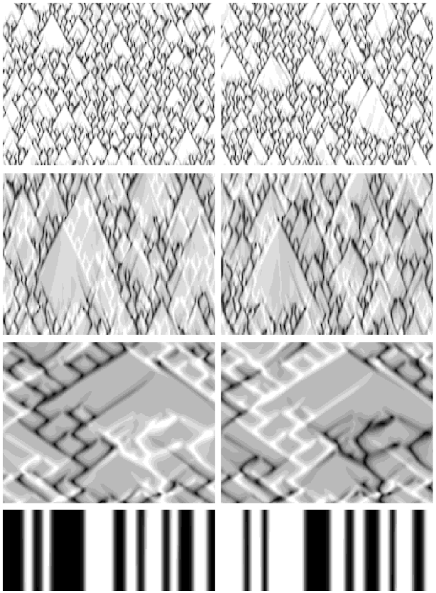
FIG. 1.: Space-time plot ot the modulus $|A_{1}|$ (left) and $|A_{2}|$ (right) for four values of the coupling parameter $\gamma$: From top to bottom, $\gamma=0.1,0.5,0.95$ and $1.05$. The horizontal axis represents space and the vertical axis time (2000 time units for $\gamma=0.95$, 100 for $\gamma=1.05$ and 200 in the other two plots). The grey levels change linearly from the minimum (black) to the maximum (white) of the modulus. The parameters are $\mu=1$, $\alpha=0.2$ and $\beta=-2.0$. For $\gamma=0.1$, the structures appearing in $|A_{1}|$ and $|A_{2}|$ are almost independent. However, for $\gamma=0.5$, the defects in $|A_{1}|$ (black and white structures) becomes slightly synchronized with the defects in $|A_{2}|$ and, for $\gamma=0.9$, the synchronization is almost complete.

In the optical interpretation of (2) the laminar regions with $|A_{1}|=|A_{2}|$ corresponds to transverse domains of linearly polarized light, although with a random direction of linear polarization. The localized structures are essentially circularly polarized objects since one of the two amplitudes dominates over the other. Around these structures the plane wave solutions with $|A_{1}|\neq|A_{2}|$ have different frequencies, so that they correspond to depolarized solutions of (2) [15]. As $\gamma>1$, localized traveling structures dissapear and one is left with circularly polarized domains separated by polarization walls.

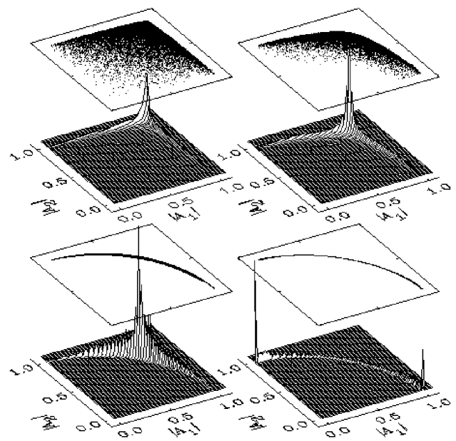
FIG. 2.: Comparison of the states reached at long times starting from noise for (from left to right, and from top to bottom) $\gamma=0.1,0.5,0.95$ and $1.05$. The joint probability distribution $p(|A_{2}|,|A_{1}|)$ is shown as a 3D surface. The vertical scale is arbitrary, the same in the first three plots and three times larger for $\gamma=1.05$. On top of each surface, $|A_{1}(x,t)|$ vs $|A_{2}(x,t)|$ are shown in the form of a dotted plot obtained from the values of $|A_{1}|$ and $|A_{2}|$ at space-time points during a time interval of 50 units.

It is usually argued that for $\gamma>1$ the dynamics of the coupled CGLE (2) is well represented by a single CGLE since only one of the two waves survives. This is certainly not true in the STI domain of parameters considered here since a single CGLE would give rise to STI dynamics whereas the coupled set (2) does not for $\gamma>1$. In general a description in terms of a single CGLE would not be reliable for parameter values at which the single amplitude dynamics produces amplitude values close to zero.

We next show that the correlations observed for increasing $\gamma$ in Fig. 1 are in fact a kind of spatiotemporal synchronization, in the generalized sense defined in [11, 12]. To this end a characterization of the synchronizing process can be given by analyzing the joint distribution of the two variables. This distribution and values of $|A_{1}|$ versus $|A_{2}|$ are plotted in Fig.2. The cloud of points correspond to the different space–time points of Fig. 1. For $\gamma<<1$ we obtain a diffuse cloud of points indicating essentially independent dynamics. The concentration of points around $|A_{1}|^{2}=|A_{2}|^{2}=\mu/(1+\gamma)$ corresponds to the laminar regions, but excursions away from that solution are independent. As the coupling is increased with $\gamma<1$ the cloud of points approaches the curve given by $|A_{1}|^{2}+|A_{2}|^{2}=\mu$. This indicates synchronization of the dynamics of structures departing from the laminar regions. The points with larger values of $|A_{1}|$ and smaller values of $|A_{2}|$ (and vice versa) correspond to the localized traveling structures. Intermediate points among these ones and those around $|A_{1}|=|A_{2}|$ correspond to the regular solutions of non-zero wavenumber that surround the localized structures. The special case of marginal coupling is discussed below, but as we enter into the strong coupling situation ($\gamma>1$) the cloud of points concentrates in the regions $|A_{1}|^{2}=\mu$, $|A_{2}|=0$ and $|A_{2}|^{2}=\mu$, $|A_{1}|=0$, while intermediate points correspond to the domain walls separating these ordered regions. It should be pointed out that we are considering just the modulus of the complex fields $A_{1,2}$. The coupled phase dynamics does not show synchronization, at least not in an obvious manner, so that we are in a case of partial synchronization as considered in [20].

A quantitative measure of the synchronizing process can be given in terms of information measures [21]. The entropy $H(X)=-\sum_{x}p(x)\ln p(x)$, where $p(x)$ is the probability that $X$ takes the value $x$, measures the randomness of a discrete random variable $X$. For two random discrete variables, $X$ and $Y$, with a joint probability distribution $p(x,y)$, the mutual information $I(X,Y)=-\sum_{x,y}p(x,y)\ln[p(x)p(y)/p(x,y)]$ gives a measure of the statistical dependence between both variables, the mutual information being $0$ if and only if $X$ and $Y$ are independent. Considering the discretized values of $|A_{1}|$ and $|A_{2}|$ at space-time points as random variables $X=|A_{1}|$, $Y=|A_{2}|$, their mutual information is a measure of their synchronization. In Fig. 3(left) we have plotted the mutual information and the entropy of $|A_{1}|$ and $|A_{2}|$ as a function of $\gamma$ [22]. This graph shows that the entropy of $|A_{1}|$ and $|A_{2}|$ remains constant for increasing values of $\gamma$, so that increasing $\gamma$ does not reduce the uncertainty associated with the single-point distributions of $A_{1,2}$. This indicates that synchronization is not here the result of reduced randomness due to the increase of time and length scales observed in Fig. 1. However, the larger is $\gamma$ the larger becomes the mutual information, approaching its maximum possible value ($I=H(|A_{1}|)=H(|A_{2}|)$) as $\gamma\rightarrow 1$. An additional quantitative measurement of synchronization is given by the linear correlation coefficient $\rho=(\langle|A_{1}||A_{2}|\rangle-\langle|A_{1}|\rangle\langle|A_{2}|\rangle)(var(|A_{1}|)var(|A_{2}|))^{-1/2}$ with $var(x)$ being the variance of $x$. This coefficient, plotted as a function of $\gamma$ in Fig. 3 (right), is negative indicating that when $|A_{1}|$ increases, $|A_{2}|$ decreases, and vice versa.

Our quantitative indicators of synchronization, $I$ and $\rho$, approach their maximum absolute values as $\gamma\rightarrow 1$. We also observe that the regime of coupled STI disappears for $\gamma>1$. In fact, the generalized synchronization observed, manifested by the tendency of the space-time signals towards the functional relation $|A_{1}|^{2}+|A_{2}|^{2}=\mu$, is probably related to the fact that for $\gamma=1$ this is an attracting manifold for homogeneous states: Writing (2) in terms of $R^{2}\equiv|A_{1}|^{2}+|A_{2}|^{2}$ and $\chi\equiv\arctan(|A_{1}|/|A_{2}|)$, it is immediate to see that homogeneous solutions for $\gamma=1$ are $R^{2}=\mu$ and $\chi$ arbitrary. To understand the preference for these solutions it is instructive to look at the transient dynamics starting from random initial conditions: $R(x,t)$ has a very fast evolution towards $R=\sqrt{\mu}$ with no regime of STI existing at any time. During this fast evolution, the phase $\chi(x,t)$ covers almost completely the range of its possible values. The late stages of the dynamics are characterized by a spatial diffusion of the phase $\chi(x,t)$ until it reaches a space-independent arbitrary value $\chi(x,t)=\chi_{0}$. In a $|A_{1}|$ vs $|A_{2}|$ dotted plot as the ones in Fig. 2 this is visualized by a cloud of points quickly approaching $R^{2}=\mu$ and then collapsing into a single point. Runs with different random initial conditions lead to different $\chi_{o}$. An underlying reason for the special dynamical behavior at $\gamma=1$ is the separation of time scales for $R$ and $\chi$. For $\gamma\neq 1$, the zero wavenumber components of $R$ and $\chi$ have a nonzero driving force and they compete dynamically but, at $\gamma=1$, $\chi(k=0)$ is a marginal variable, while $R(k=0)$ is strongly driven. As a consequence, $R$ relaxes quickly towards $R^{2}=\mu$. Once $R$ becomes space-homogeneous, the different wavenumber components of $A_{1,2}$ are decoupled and the zerowavenumber solution wins by diffusion of $\chi$.

FIG. 3.: Left: Entropy of $|A_{1}|$ ($\Box$) and $|A_{2}|$ ($\bigtriangleup$) and their mutual information I ($\diamond$) as a function of $\gamma$. Right: Correlation coefficient $\rho$ of $|A_{1}|$ vs $|A_{2}|$ as a function of $\gamma$.

In some of our simulations the STI regime has been observed to disappear for a coupling smaller than $\gamma=1$, but this seems to be a consequence of finite-size effects: The size of the laminar portions of Fig.(1) increases with the coupling $\gamma$. When this size becomes similar to system size, one of the stable plane waves can occupy the whole system, thus preventing any further appearance of defects and STI. For a given initial condition, with parameters $\alpha=0.2$ and $\beta=-1.4$, and a system size $L=512$ the STI regime was seen to disappear at $\gamma=0.85$. As soon as the system size was doubled the STI regime reappeared again. By reducing system size to $L=256$ the STI regime disappeared for smaller $\gamma$. The conclusion from this an other numerical experiments is that STI exists for all $\gamma<1$ in the same range of parameters as it exists in the single CGLE, with time and length scales diverging as $\gamma$ approaches $1$, where STI disappears.

In summary we have described a regime of synchronized STI dominated by the space-time synchronization of localized structures. Synchronization is measured by a mutual information and a correlation parameter that take their absolute maximum value at the boundary between weak and strong coupling $\gamma=1$. Beyond this boundary ($\gamma>1$) STI disappears but the strong, coupled system dynamics cannot be described in terms of a single dominant amplitude.

Financial support from DGICYT Project PB94-1167 (Spain) and European Union Project QSTRUCT (FMRX-CT96-0077) are acknowledged. R.M. also acknowledges partial support from the PEDECIBA and CONICYT (Uruguay).

REFERENCES

- [1]
- [2] On leave from Universidad de la República (Uruguay).
- [3] http://www.imedea.uib.es/nonlinear.
- [4] M. Cross and P. Hohenberg, Science 263; 1569 (1994). M. Dennin, G. Ahlers, and D. S. Cannell, Science 272, 388 (1996); R. Ecke, Y. Hu, R. Mainieri, and G. Ahlers, Science 269, 1704 (1995).
- [5] L. M. Pecora and T. L. Carrol, Phys. Rev. Lett. 64, 821 (1990); P. Colet and R. Roy, Opts. Lett. 19, 2056 (1994).
- [6] C. Huygens, J. des Scavans (1665); K. Wiesenfeld, P. Colet, and S. H. Strogatz, Phys. Rev. Lett. 76, 404 (1996).
- [7] B. Shraiman et al., Physica D 57, 241 (1992).
- [8] H. Chaté, Nonlinearity 7, 185 (1994).
- [9] M. Caponeri and S. Ciliberto, Physica D 58, 365 (1992).
- [10] R. Montagne, E. Hernández-García, and M. San Miguel, Phys. Rev. Lett. 77, 267 (1996); Physica D 96, 47 (1996)
- [11] N. F. Rulkov, M. M. Sushchik, L. S. Tsimring, and H. D. I. Abarbanel, Phys. Rev. E 51, 980 (1995).
- [12] L. Kocarev and U. Parlitz, Phys. Rev. Lett. 76, 1816 (1996).
- [13] M. Cross and P. Hohenberg, Rev. Mod. Phys. 65, 851 (1993), and references therein.
- [14] W. van Saarloos and P. Hohenberg, Physica D 56, 303 (1992), and (Errata) Physica D 69, 209 (1993).
- [15] M. San Miguel, Phys. Rev. Lett. 75, 425 (1995).
- [16] A. Amengual, D. Walgraef, M. San Miguel, and E. Hernández-García, Phys. Rev. Lett. 76, 1956 (1996).
- [17] H. Chaté, in Spatiotemporal Patterns in Nonequilibrium Complex Systems, Vol. XXI of Santa Fe Institute in the Sciences of Complexity, edited by P. Cladis and P. Palffy-Muhoray (Addison-Wesley, New York, 1995), pp. 5–49.
- [18] Our numerical integration is performed by a second order pseudospectral method described elsewhere [23]. The numerical results presented in this paper have been obtained, except when indicated explicitly, for , and, without loss of generality, . The initial condition is white Gaussian noise with a mean squared amplitude at each point of . In Fig. 1, the same initial condition is taken for all values of .
- [19] S. Popp et al., Phys. Rev. Lett. 70, 3880 (1993).
- [20] M. G. Rosenblum, A. S. Pikovsky, and J. Kurths, Phys. Rev. Lett. 76, 1804 (1996).
- [21] R. J. McEliece, The theory of information and coding : a mathematical framework for communication, Vol. III of Encyclopedia of Mathematics and its Applications (Addison-Wesley, New York, 1977).
- [22] To calculate and we have discretized the range of possible values in bins. Therefore, the maximum possible entropy is .
- [23] R. Montagne, E. Hernández-García, A. Amengual, and M. San Miguel, (1996), to be published.