Fractal Basins of Attraction Associated with a Damped Newton’s Method

Abstract

An intriguing and unexpected result for students learning numerical analysis is that Newton’s method, applied to the simple polynomial $z^{3}-1=0$ in the complex plane, leads to intricately interwoven basins of attraction of the roots. As an example of an interesting open question that may help to stimulate student interest in numerical analysis, we investigate the question of whether a damping method, which is designed to increase the likelihood of convergence for Newton’s method, modifies the fractal structure of the basin boundaries. The overlap of the frontiers of numerical analysis and nonlinear dynamics provides many other problems that can help to make numerical analysis courses interesting.

1 Introduction

Numerical analysis is an immensely exciting area of research with many intellectual and practical benefits and yet this excitement sometimes doesn’t come across in courses and textbooks. One reason is that courses and texts sometimes do not indicate some of the frontiers of the field and why these frontiers are interesting. Perhaps more importantly, few introductory courses and texts make students aware that they are actually close to, and can contribute to, research frontiers even while participating in an introductory course. The ease of finding and exploring new problems in numerical analysis is one of its particular attractions.

As an illustration of this point that we hope will be of pedagogical interest to those teaching and thinking about numerical analysis, we pose and partially solve a question that was raised by the attractive cover picture of the book by Kincaid and Cheney [6]. (This book has been used at Duke University for the last few years in its graduate introductory course on numerical analysis; the first author was a recent student in this course when it was taught by the second author.) This cover picture is reproduced in Fig. 1

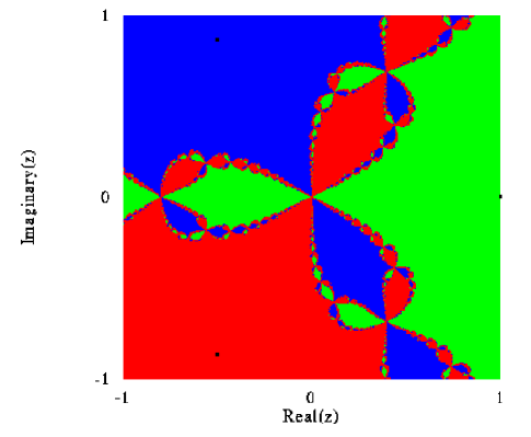
Fig. 1: The regions of three different colors indicate the approximate basins of attraction for the three roots of the complex polynomial $z^{3}-1=0$ in the square region defined by $-1\leq Real(z)\leq 1$ and $-1\leq Imag(z)\leq 1$. The positions of the roots of unity are indicated by the small black squares. This figure was computed numerically by using a mesh of $1000\times 1000$ pixels inside this square. The center point of each pixel was used to start a Newton iteration under Eq. (1). The pixel was assigned a particular basin color if convergence to a root was identified within 1000 iterations. The criterion for convergence was that both the magnitudes of the correction $z_{i+1}-z_{i}$ and of the residual $z_{i}^{3}-1$ were smaller than the value $10^{-12}$. The boundaries separating the basins are intricately braided, with a fractal dimension of $D\approx 1.42$.

and reveals a remarkable result that is now nearly 120 years old [1, 9, 2]: for the simple polynomial equation $z^{3}-1=0$ in the complex plane, the sets of points $z_{0}$ that converge to a root under the map given by Newton’s method,

$$z_{i+1}=z_{i}-\left({z_{i}^{3}-1}\over 3z_{i}^{2}\right).$$ (1)

have an unexpected intricate geometric complexity. In the language of nonlinear dynamics [13], the set of points that converge towards a fixed point under successive iterations of some mapping is called the basin of attraction of that fixed point. Fig. 1 then says graphically that the basins of attraction for Newton’s method are bounded by intricately braided objects. Naively, one would have expected the basins of attraction to be given by the sets of points closest to a given root and so bounded by straight lines.

This braided structure is typical of geometric objects known as fractals [13, 2]. The concept of a fractal is hard to define rigorously [7] but can be casually defined as a scale-invariant set that has a non-integer dimension $D$ known as its fractal dimension. For Fig. 1, scale invariance corresponds to the fact that if any small region of the braided structure is greatly magnified, further braided structure is found of a similar complexity and there is no end to this intricate detail upon further and further magnification. The fractal dimension is perhaps best understood as a scaling exponent that generalizes the usual concept of dimension to non-integer values [13]. E.g., one kind of fractal dimension known as the capacity $C$ indicates the scaling $N_{\varepsilon}\propto\varepsilon^{-C}$ as $\varepsilon\to 0$ of the minimum number of balls $N_{\varepsilon}$ of radius $\varepsilon$ needed to cover the set as the ball radius $\varepsilon$ tends to zero. Numerical calculations of the capacity of a set are often slowly convergent when the points of the set are visited with non-uniform probability (measure) by the dynamics [4]. For this reason, in the following we have used the average pointwise dimension $D$ [8] to quantify the structure of the fractal basin boundaries. This dimension takes into account the probability of visiting different parts of a set and so is more rapidly convergent in practice..

Another interesting aspect of the fractal structure in Fig. 1 is that the boundaries satisfy the counterintuitive Wada property [10]: every point on the boundary of one basin of attraction is also on the boundary of the other basins of attraction.

The Kincaid and Cheney book touches only briefly on these remarkable facts and does not mention that fractal basins are in fact typical for Newton methods, rather than rare or pathological. Some of the important (and largely numerical) discoveries in the field of nonlinear dynamics in the last twenty years is that fractal structures pop up over and over again for nonlinear equations and for typical choices of equation parameters and of initial conditions: basin boundaries can be fractal, the attracting limit set for maps, flows, and partial differential equations can be fractal, and the set of parameter values that lead to a particular class of solutions (e.g., fixed points) can be fractal [13]. This fractal structure has important practical implications for many numerical problems and algorithms and so numerical analysis students should be aware of this. As one example, fractal basins of attraction for Newton’s method imply that it will generally be difficult or impractical to characterize the ever-so-important initial guesses that will lead to convergence. In some extreme cases, it may be impossible to characterize the dependence of the algorithm or even of a laboratory experiment on parameters [11].

Fig. 1 is a good example of a result that is easily computed by students in an introductory numerical analysis course and that leads to interesting, and largely unexplored, questions that might entice a student to get interested in numerical analysis. Thinking about this figure carefully raises the following kinds of questions: Are fractal boundaries associated with Newton’s method rare or common? What determines the braided geometric structure (e.g., its fractal dimension $D$)? Do other root-finding algorithms lead to such fractal structure and, if so, can one relate the details of the algorithm to the fractal geometry? How do floating point errors affect the fractal structure? What are the implications of these fractal basin boundaries for root-finding software?

In the following, we address briefly one of the above questions, namely do different root-finding algorithms—particularly Newton’s method with damping—also lead to fractal basins of attraction? A well known weakness of Newton’s method is that it is locally, but rarely globally, convergent [6]. To improve this situation, researchers have invented damping methods [5, 3] that try to increase the likelihood that an initial condition will lead to convergence. The basic strategy of most damping methods is to add only a fraction of a Newton step when correcting the current estimate of a root. During successive iterations, the damping algorithm usually increases the fraction of the Newton step towards the value of one until full Newton steps are taken and quadratic convergence is achieved.

A question which, to our knowledge, seems not to have been discussed previously is then this: for fixed points with fractal basins of attraction, do damping methods change the fractal structure? If so, do they diminish or increase the fractal dimension $D$ of the boundaries? An interesting related question is whether damping works by increasing the basin of attraction, in that the basin with damping strictly contains the basin without damping. An increase in the fractal dimension $D$ would possibly be an undesirable effect since more initial conditions would lie near the boundaries, making it harder to find criteria for identifying good initial conditions, which is often the most challenging part of a Newton method for many scientific problems. The question of how damping may modify the fractal basins of attraction is a natural one to ask given material normally covered in an introductory numerical analysis course and is also within the ability of students to investigate themselves.

2 The Fractal Basins Associated with Armijo’s Rule

To study numerically and graphically how the basins of attraction may be modified by damping, we consider one of the simplest damping methods, the Armijo rule [5, 3]. For the equation $z^{3}-1=0$, the Armijo rule modifies the Newton algorithm (1) by introducing a fractional damping coefficient $1/2^{j}$ in front of the Newton step as follows:

$$z_{i+1}=z_{i}-{1\over 2^{j}}\left(z_{i}^{3}-1\over 3z_{i}^{2}\right),$$ (2)

where $j$ is a nonnegative integer. Before the approximate root $z_{i}$ is corrected to give a new and hopefully better estimate $z_{i+1}$, the integer $j$ is increased from zero (i.e., the fraction of the step added is decreased) until the following criterion is just satisfied:

$$\left|z_{i+1}^{3}-1\right|\leq\left(1-{1\over 2^{j+1}}\right)|z_{i}^{3}-1|.$$ (3)

At this point, $z_{i+1}$ is computed from Eq. (2) with the given value of $j$ and the Newton method is iterated until convergence or some maximum limit of iterations is attained. (If the latter, then usually a new initial condition must be tried.) Under certain assumptions of smoothness, one can prove that the Armijo method is guaranteed to converge to some root [3].

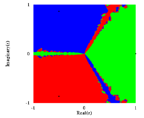
Fig. 2: Plot of the basins of attraction of the roots of the equation $z^{3}-1=0$ under Armijo’s rule, Eqs. (2) and (3), calculated in the same way as described in Fig. 1. The fractal structure is preserved and slightly modified by damping when compared with Fig. 1. The basin boundaries have a fractal dimension $D\approx 1.29$ with a standard deviation of $0.02$ as determined from a least-squares fit to a plot of $\log(P_{\varepsilon})$ versus $\log(1/\varepsilon)$ (not shown).

A comparison of the basins of attraction of the Newton-Armijo algorithm (Fig. 2) with those of the Newton algorithm (Fig. 1) yields several interesting insights. First, the basin boundaries are not smoothed out under damping but retain a fractal structure. Second, although the basins themselves are substantially altered (there are larger contiguous regions of a given color in Fig. 2 compared to Fig. 1), damping causes only a modest change in the basin boundaries as quantified by the fractal dimension $D$. The dimension of the fractal boundaries in Fig. 2 is $D\approx 1.29$ whereas the fractal dimension in Fig. 1 has the somewhat larger value 1.42. The approximately ten percent relative decrease in the dimension seems consistent with the expected smoothing effect arising from the Armijo factor $1/2^{j}$ at each Newton-like step. Nevertheless, the dimension of the basin boundary does not generally decrease under damping as we point out in the next section.

3 A Less Symmetric Example

Our discussion for the polynomial $z^{3}-1=0$ is somewhat atypical in that there are only three roots and the corresponding basins of attraction are related by symmetry rotations around $z=0$. To explore a more representative example and to suggest the rich geometric changes that damping can induce, we have also studied numerically the approximate basins of attraction of Newton and Newton-Armijo algorithms for the following two-dimensional nonlinear system:

$${x-\sin(x)\cosh(y)} = {0,}$$

$${y-\cos(x)\sinh(y)} = {0,}$$

which the second author first came across in a collection of numerical analysis problems [12, page 559, problem 16.86].

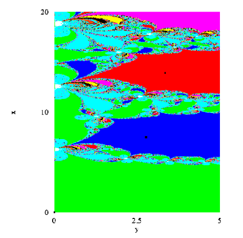
Fig. 3: Plot of the basins of attraction of the solutions of the system of equations (LABEL:eq:Complex) under Newton’s method. Seven of the colors (green, purple, red, magenta, orange, yellow, and black) represent seven different basins of attraction (the most spatially extended regions). The blue regions represents all other basins while the white regions represent starting points for which the iterative process did not converge within 1000 iterations. The figure was calculated using a mesh of $1500\times 1500$ pixels spanning the spatial region $0\leq x\leq 20$ and $0\leq y\leq 5$. The three solutions that lie inside this region are shown by the small black squares and have approximate coordinates $(x,y)=(0,0)$, $(7.5,2.8)$, and $(13.9,3.4)$ respectively. The fractal dimension of the boundary of the magenta-colored basin (belonging to the approximate solution $(x,y)=(20.2,3.7)$) is $D\approx 1.38\pm 0.04$ as determined from a least-squares fit to a plot of $\log(P_{\varepsilon})$ versus $\log(1/\varepsilon)$.

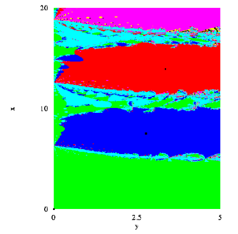
Fig. 4: The approximate basins of attraction of the solutions of Eq. (LABEL:eq:Complex) under Armijo’s rule, using the same coloring scheme, resolution, and convergence criteria as in Fig. 3. The fractal dimension of the boundary of the magenta-colored basin colored is unchanged within numerical accuracy.

Figures 3 and 4 reveal a dramatic change in the shape and number of basins of attraction under damping although, within our numerical accuracy, the fractal dimension of a particular basin (the magenta basin belonging to the root $(x,y)=(20.2,3.7)$) is unchanged with a value $D\approx 1.4$.

Using starting points centered on $1500\times 1500$ pixels spanning the region $0\leq x\leq 20$ and $0\leq y\leq 5$, we found that Newton’s method converged towards $120$ different solutions Some of these solutions are shown in Fig. 5 and are color coded to indicate the associated basin of attraction. In contrast, the same initial conditions with Armijo’s rule yielded only $53$ different solutions, a substantially smaller number. These solutions were a subset of the 120 solutions obtained using Newton’s method.

Figures 3-5 raise fascinating open questions in addition to those already discussed above in the context of Fig. 1. As an example, what has happened to the many basins of attraction that are now missing in the damped algorithm (53 solutions versus 120 for initial conditions in a certain given region)? Does the Wada property still apply to the various basins and, if so, which basins are linked by a given boundary? If not all basins are linked by the Wada property, do the different basin boundaries have different fractal dimensions and, if so, what determines these different dimensions?

Finally, one can again ask how the geometry in Fig. 4 might depend on the damping algorithm. A canonical and interesting choice to study would be continuous damping in the sense of using an infinitesimal damping factor $ds$ along a Newton direction. (We are indebted to our colleague, Dr. Donald Rose, for this suggestion.) Instead of iterating an Armijo-Newton map similar to Eqs. (2) and (3), one would then integrate a system of $N$ ordinary differential equations given by:

$${d{\bf X}\over ds}=-{\bf J}^{-1}\cdot{\bf F}({\bf X}),$$ (5)

where the $N$-dimensional system of equations is given by ${\bf F}({\bf X})=0$, where ${\bf J}({\bf X})$ is the $N\times N$ Jacobian matrix ${\bf J}({\bf X})=\partial{\bf F}/\partial{\bf X}$, and where $s$ is some arbitrary continuous parameter. Starting from some initial guess ${\bf X}_{0}$, numerical integration of Eq. (5) will generate a path ${\bf X}(s)$ that must end up at a solution provided the Jacobian matrix remains nonsingular along this path. Challenging questions are raised in this continuous case: how long one must integrate to get close to a root? What integration accuracy is needed? What numerical algorithms should be used? What are the basins of attraction and are they fractal?

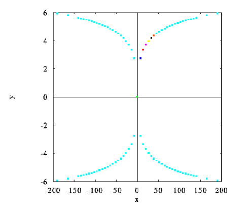
Fig. 5: Plot of some of the solutions of the system of equations (LABEL:eq:Complex) under Newton’s method, using the same coloring scheme, resolution, and convergence criteria as in Fig. 3. All the solutions obtained under Armijo’s rule were also obtained undere Newton’s method; the basins of the solutions are nevertheless different. The color coding of the roots agrees with the color of the basins in Fig. 3 and Fig. 4.

4 Conclusions

Numerical analysis is an exciting and attractive subject specifically because it is fairly easy to to investigate novel problems even at the level of an introductory course. As an illustration of this, we have investigated numerically and graphically the problem of how a simple damping algorithm for Newton’s method, Armijo’s rule, modifies the fractal basins of attraction found for the complex polynomial $z^{3}-1=0$ . We have also investigated a less symmetric and perhaps more general case, Eq. (LABEL:eq:Complex), in which the basins of attraction are fundamentally changed upon damping. Our goal here was not to present a detailed or complete analysis but instead to suggest how students learning numerical analysis can easily find and explore new problems. The field of nonlinear dynamics [13] raises many related questions of geometric structure and their relation to numerical algorithms and is a valuable source of other ideas of pedagogical value for courses in numerical analysis.

References

- [1] A. Cayley, The Newton-Fourier imaginary problem, American J. of Mathematics, 2 (1879), p. 97.
- [2] R. M. Crownover, Introduction to Fractals and Chaos, Jones and Bartlett, Boston, 1995.
- [3] J. E. Dennis and R. Schnabel, Numerical Methods for Unconstrained Optimization and Nonlinear Equations, Prentice-Hall, Englewood Cliffs, NJ, 1983.
- [4] H. S. Greenside, A. Wolf, J. Swift, and T. Pignataro, Impracticality of a box-counting algorithm for calculating the dimensionality of strange attractors, Phys. Rev. A, 25 (1982), pp. 3453–3456.
- [5] W. Hager, Applied Numerical Linear Algebra, Prentice-Hall, Englewood Cliffs, NJ, 1988.
- [6] D. Kincaid and W. Cheney, Numerical Analysis, Brooks/Cole, Pacific Grove, California, second ed., 1991.
- [7] B. B. Mandelbrot, The Fractal Geometry of Nature, W. H. Freeman, New York, 1983.
- [8] F. C. Moon, Chaotic vibrations : an introduction for applied scientists and engineers, Wiley, New York, 1992.
- [9] M. Nauenberg and H. J. Schellnhuber, Analytical evaluation of the multifractal properties of a Newton Julia set, Phys. Rev. Lett., 62 (1989), pp. 1807–1810.
- [10] H. E. Nusse and J. A. Yorke, Basins of attraction, Science, 272 (1996), pp. 1376–1380.
- [11] E. Ott, J. C. Alexander, I. Kan, J. C. Sommerer, and J. A. Yorke, The transition to chaotic attractors with riddled basins, Physica D, 76 (1994), pp. 384–410.
- [12] F. Scheid, 2000 Solved Problems in Numerical Analysis, Schaum’s Solved Problem Series, McGraw-Hill, New York, 1990.
- [13] S. H. Strogatz, Nonlinear Dynamics and Chaos, Addison-Wesley, Reading, MA, 1994.