Characterization of Landau$-$Zener Transitions
in Systems with Complex Spectra

Abstract

This paper is concerned with the study of one-body dissipation effects in idealized models resembling a nucleus. In particular, we study the quantum mechanics of a free particle that collides elastically with the slowly moving walls of a Bunimovich stadium billiard. Our results are twofold. First, we develop a method to solve in a simple way the quantum mechanical evolution of planar billiards with moving walls. The formalism is based on the scaling method [1] which enables the resolution of the problem in terms of quantities defined over the boundary of the billiard.
The second result is related to the quantum aspects of dissipation in systems with complex spectra. We conclude that in a slowly varying evolution the energy is transferred from the boundary to the particle through Landau$-$Zener transitions.

^aDivision de Physique Théorique, Institut de Physique Nucléaire.
91406, Orsay Cedex, France.
^bDepartamento de Física, Facultad de Ciencias Exactas y Naturales,
Universidad de Buenos Aires. Ciudad Universitaria, 1428 Buenos Aires, Argentina.
^cDepartamento de Física, Comisión Nacional de Energía Atómica.
Av. del Libertador 8250, 1429 Buenos Aires, Argentina.

Introduction

The way in which energy is transferred from the time dependent mean field to the individual nucleons is an important ingredient, for instance, in fission processes [2] and in large amplitude collective motion at low energies. Because of the Pauli principle it is expected that one body effects, i.e., loss of energy due to collision of independent individual nucleons with the mean field, should dominate the dissipation mechanism.
Several descriptions of these processes involving different approximations are available in the literature [3, 4, 5, 6]. These theories are perturbative in character and linear in the collective motion. Therefore they are not suited to address the issues related to nonlinear dynamics and the onset of chaos. On the other hand, the integrable or chaotic nature of the motion is of crucial importance to the dissipation mechanism [7],i.e., the transition from order to chaos provides the possibility for a variety of nuclear responses (from elastic to elastoplastic to dissipative). Therefore detailed studies of simplified models resembling a nucleus may be of interest.
Planar billiards are perhaps the best systems to model the processes described above in which the nucleus can be imagined as a time-dependent container filled with a gas of non interacting point particles [3, 8]. Billiard systems have been thoroughly studied in the context of classical and quantum chaos [9]. In particular it has been shown that the quantum spectra of generic planar billiards have GOE (Gaussian Orthogonal Ensemble) characteristics that are observed in the excited spectra of nuclei [10].
In a seminal paper, Hill and Wheeler [11] suggested the Landau$-$Zener (L-Z) transitions as a mechanism for nuclear dissipation. The mechanism is based on the excitation of the individual nucleons via transitions at avoided level crossings near the Fermi surface. These excitations produce the damping of collective motion describing deformation of the nucleus. In an adiabatic evolution of the collective coordinates, the nucleus changes its shape relatively slowly, while the nucleonic levels move up and down in energy. Small deformations in the nuclear shape produce occasionally that two nucleonic levels almost cross each other and experience an avoided crossing. During the whole process many avoided crossings occur with more or less random transitions between nearest neigbours, in such a way that the system may end up in an arbitrary energy state. Within this picture one can imagine a stochastic dynamics in which by simply reversing the temporal evolution one does not recover the initial state. Therefore, the internal degrees of freedom are excited and the motion of the collective coordinates is thus damped.
More recently Wilkinson, making good use of the properties of complex spectra, introduced a statistical treatment of dissipation in finite-sized quantum systems in terms of L-Z transitions in the context of random matrix theory [12]. However, a L-Z mechanism as the generator of dissipation in systems with complex spectra, has recently been seriously questioned [13]. In their works Bulgac and collaborators suggest that the diffusive process in energy is dominated by memory effects and that the picture for dissipation through L-Z transitions is likely to be incorrect (see section III for a detailed analysis of these arguments).
Obviously the best way to elucidate this question is to solve the quantum mechanical evolution of a generic system, though this is difficult even for planar billiards with moving walls.

The goal of the present article is to present a new formulation to solve the quantum mechanical evolution of planar billiards with moving boundaries. Using this formulation we study the time evolution of a specific billiard, the Bunimovich Stadium with externally driven walls. We restrict the analysis to slowly varying (adiabatic) evolutions [14]. The notion of slow motion will be quantified in section IV. Our aim is to understand whether a L-Z mechanism generates the damping of the slow degree of freedom in a system with complex spectra.

The work outline is as follows. In the next section we introduce a one-dimensional new formulation in order to solve the quantum evolution of planar billiards with moving walls . Section II is devoted to the numerical results obtained for the Bunimovich Stadium billiard with GOE spectrum characteristics. Using these results, we evaluate relevant properties for the dissipation process. In section III we discuss in detail whether a L-Z transition mechanism describes the dissipation of the slow degree of freedom or equivalently the difussion of the fast ones. The last section is devoted to final remarks and conclusions.
Before proceeding we want to stress that planar billiards systems externally driven can also be used to model other problems often encountered for example in mesoscopic systems, atomic clusters and of course deformable cavities [15]. Therefore, the results presented in this work could also contribute to domains other than nuclear physics.

I The Method

In a recent work Vergini and Saraceno developed a method to calculate directly all eigenvalues and eigenfunctions in a narrow energy range of quite general time independent $2-d$ billiards, by solving a generalized eigenvalue problem in terms of quantities defined over the boundary. The method is based on the use of scaling that enables to write the boundary norm explicitly as a function of the energy [1].
The aim of this section is to extend the method of scaling to solve the Schrödinger equation for $2\!-\!d$ billiards with time dependent boundary conditions.
Let ${\cal C}(t)$ be a closed curve defining at time $t$ a two dimensional domain ${\cal D}(t)$. We restrict to star shaped domains, this means that $r_{n}\equiv{\bf r}.{\bf n}>0\;\forall{\bf r}\in{\cal C}(t);\;{\bf n}$ is the outgoing normal to ${\cal C}(t)$. Consider a particle of mass $m$ inside the billiard, then the Schrödinger equation reads,

$${\partial{\Psi}\over\partial{t}}=i\frac{\hbar}{2m}\Delta\Psi\;.$$ (1)

$\Psi$ satisfies the time dependent boundary condition $\Psi({\bf\zeta},t)=0$ where ${\bf\zeta}$ is a point on ${\cal C}(t)$, and we consider functions normalized to one on the domain. A standard procedure is to expand the solution in terms of the adiabatic basis,

$$\Psi({\bf r},t)=\;\sum_{\mu}a_{\mu}(t)\;P_{\mu}(t)\;\phi_{\mu}({\bf r},t)\;.$$ (2)

$\;P_{\mu}(t)\equiv\exp(-i\int_{0}^{t}\omega_{\mu}dt^{\prime})\;$ is the contribution of the dynamical phase with $\omega_{\mu}=\hbar k_{\mu}^{2}(t)/\;2m$. The adiabatic basis $\;\{\phi_{\mu}\}\;$ constitutes a complete set of real eigenfunctions of the billiard at each time; that is, $\phi_{\mu}$ satisfies the Helmholtz equation $\Delta\phi_{\mu}({\bf r},t)=-k_{\mu}^{2}(t)\phi_{\mu}({\bf r},t)$ with Dirichlet boundary condition $\phi_{\mu}({\bf\zeta},t)=0$, and it is a continuous function of time.
We generate from the original domain defined by ${\cal C}(t)$ a family of systems that depends on a parameter $\alpha$. These systems evolve with the curves ${\cal C}_{\alpha}(t)$ that are obtained from ${\cal C}(t)$ through a scaling transformation on the plane ${\bf r}\rightarrow\alpha{\bf r}$ (if ${\bf\zeta}$ is a point on ${\cal C}(t)$, then ${\bf\zeta}/\alpha$ is the corresponding point on ${\cal C}_{\alpha}(t)$).
To each function $\phi_{\mu}({\bf r},t)$ we associate the scaling function $\phi_{\mu}(\alpha,{\bf r},t)\equiv\phi_{\mu}(\alpha{\bf r},t)$. This family of functions depending on the scaling parameter $\alpha$ verifies the Helmholtz equation with wave number ${\alpha}k_{\mu}$ and satisfies the Dirichlet condition over the scaled boundary. Moreover, we require that the mass of the particle in the scaled systems changes as ${\alpha}^{2}m$ in such a way that $\omega_{\mu}$ is independent of $\alpha$. The last statement implies that the time evolution is the same for all the scaled systems.
Our approach to solve the Schrödinger equation is to expand the wave function in terms of the adiabatic basis represented by the scaling functions. After replacing the expansion into the equation $(\ref{scho})$ we obtain,

$$\sum_{\nu}\dot{a}_{\nu}(t)\;P_{\nu}(t)\;\phi_{\nu}(\alpha,{\bf r},t)=\;-\sum_{\nu}a_{\nu}(t)\;P_{\nu}(t)\;{\partial\phi_{\nu}\over\partial{t}}(\alpha,{\bf r},t)\;.$$ (3)

Differentiating this equation with respect to $\alpha$ results in,

$$\sum_{\nu}\dot{a}_{\nu}(t)\;P_{\nu}(t)\;{\partial\phi_{\nu}\over\partial{\alpha}}(\alpha,{\bf r},t)=\;-\sum_{\nu}a_{\nu}(t)\;P_{\nu}(t)\;{\partial^{2}\phi_{\nu}\over\partial{\alpha}\partial t}(\alpha,{\bf r},t)\;.$$ (4)

The remainder of the calculus consists on commuting the order of the partial derivation in the rhs of $(\ref{der2})$, multiply the equation by $\;{\partial\phi_{\mu}/\partial{\alpha}}\;(\alpha,{\bf r},t)\;$ and specialize the resulting equation in $\alpha=1$. Finally we integrate over the boundary of the billiard ${\cal C}(t)$. After this straightforward calculation, the final equation reads,

$$\sum_{\nu}\dot{a}_{\nu}(t)\;P_{\nu}(t)\;\oint_{{\cal C}(t)}{\partial\phi_{\mu}\over\partial{\alpha}}{\partial\phi_{\nu}\over\partial{\alpha}}{dl\over r_{n}}=\;-\sum_{\nu}a_{\nu}(t)\;P_{\nu}(t)\;\oint_{{\cal C}(t)}{\partial\phi_{\mu}\over\partial{\alpha}}{\partial\over\partial{t}}({\partial\phi_{\nu}\over\partial{\alpha}})\;{dl\over r_{n}}\;,$$ (5)

where $dl$ is the length element on the boundary. For the sake of simplicity we have omitted the argument $(\alpha=1,{\bf r},t)$ in the last equation. In [1] it was proved that the integral in the lhs of the last equation verifies a quasiorthogonality relation, this means

$${1\over 2k_{\mu}^{2}}\oint_{{\cal C}(t)}{\partial\phi_{\mu}\over\partial{\alpha}}{\partial\phi_{\nu}\over\partial{\alpha}}{dl\over r_{n}}=\delta_{\mu\nu}+{(k_{\mu}-k_{\nu})\over(k_{\mu}+k_{\nu})}{\cal O}(1)\;.$$ (6)

Employing this important relation in (5), we derive the standard system of differential equations in the adiabatic basis

$$\dot{a}_{\mu}(t)=\;-\sum_{\nu}a_{\nu}(t)(P_{\nu}(t)/P_{\mu}(t))\;C_{\mu\nu}(t)$$ (7)

with the coefficients $C_{\mu\nu}$ computed approximately in terms of quantities defined over the boundary,

$${\it C}_{\mu\nu}(t)\simeq{1\over 2k_{\mu}^{2}}\oint_{{\cal C}(t)}{\partial\phi_{\mu}\over\partial{\alpha}}{\partial\over\partial{t}}({\partial\phi_{\nu}\over\partial{\alpha}}){dl\over r_{n}}\;.$$ (8)

The exact expression for the coefficients follows from $(\ref{auto1})$,

$$C_{\mu\nu}(t)=\int_{{\cal D}(t)}\phi_{\mu}({\bf r},t)\;{\partial\phi_{\nu}\over\partial{t}}({\bf r},t)\;d\sigma\;.$$ (9)

In the last equation each $C_{\mu\nu}(t)$ involves an integration on the domain ${\cal D}(t)$. It is also very easy to prove that they are antisymmetric.
To compute each $C_{\mu\nu}$ via the equation $(\ref{2cmunu})$ the domain of integration has to be partitioned at least in $N\approx{k}^{2}$ cells, with $k$ equal to the maximum among the wave numbers of the functions $\phi$ in the region of integration, $k=max\{k_{\mu},k_{\nu}\}$. If $n$ is the dimension of the adiabatic basis restricted to the energy region where the evolution will take place, one needs to know $n^{2}$ coefficients. As a consequence, the dimension of the problem of finding the coefficients $C_{\mu\nu}$ from equation $(\ref{2cmunu})$ turns to be of the order of $n^{2}\times N$ at each time.
As a way to check the goodness of the new formulation we have computed for the specific billiard studied in section II, the coefficients ${\it C}_{\mu\nu}$$(t=0)$ for a fixed $\mu$, with $\nu=\mu+j$ $(j=0,\pm 1,\pm 2,...)$ calculated exactly (equation (9)) and using the equation (8) (see Fig. 1). The correspondance is extremely good over a great number of levels. The departure between the two plots begins for $\mid j\mid\approx 10$, but in this region the values of the coefficients are very small.
With the present formulation the CPU time necessary to compute the coefficients is considerably reduced in comparison with the time needed in the standard approach (equation (9)). From the preceding remarks, and in order to study the interaction between neighbouring levels in the spectrum, we will calculate the coefficients $C_{\mu\nu}$ employing the relation (8).

II Numerical Results

Using the method presented in section I, we will analize the dynamics of a particle of mass $m$ inside a Bunimovich stadium billiard with moving boundaries.
A point particle inside the static stadium billiard is a very well known example of a fully classical chaotic system [20]. The particle moves freely on the two dimensional domain and is perfectly reflected from its boundary. The boundary is formed by two semi-circles of radius $r$ connected by two straight lines of length $2a$. Fig. 2 shows a desymmetrized version of the system with area $1+\pi/4$.
To study the dynamics, the parameter $\ell\equiv a/r$ is changed with a finite velocity $\dot{\ell}$ in such a way that the total area of the billiard remains unchanged. We have fixed the area to avoid a drift in the energy spectrum; this situation is characteristic of nuclear processes where the nucleonic density is approximately constant. The drift term represents a reversible change in the energy of the system and can be neglected in the analysis of an irreversible dissipation process [21]. Therefore, the dynamics of the boundary is introduced through the function $\ell(t)$.
Fig. 3 shows the spectrum of $k=\sqrt{2mE}/\hbar$ as a function of $\ell$, $1\leq\ell\leq 1.14$. We have selected the wave numbers $k_{\mu}(\ell)$ between $48.8$ and $50$ because in this region a large number of energy levels exists in a narrow portion of the spectrum. Although the properties that we are going to evaluate are characteristic of this region of the spectrum ($k\sim 50$), as we will show below, a proper scaling can be done in order to evaluate them in other energy regions.
The spectrum exhibits the typical behavior of avoided levels crossings that characterizes the energy levels as a function of a parameter for general systems without constants of motion [22]. Also, we recognize that some avoided crossings are situated on two parallel lines labeled $L3$ and $L4$ (see Fig. 3). These lines are associated to bouncing ball states with three and four low excitations respectively. These states are highly localized in the momenta space [23], therefore their interaction with neighbouring states is smaller than the interaction between delocalized generic states.

Let us analize the coefficients $C_{\mu\nu}$ which determine the quantum mechanical evolution of the system (see section I). They may be expressed in terms of the deformation parameter $\ell$, as they satisfy $\;:C_{\mu\nu}(t)=\dot{\ell}C_{\mu\nu}(\ell)$.
Fig. 4 shows the functions $\;\mid\!C_{\mu\mu+1}(\ell)\!\mid\;$ for several pairs of nearest neighbouring levels. A well defined structure of peaks is observed. The peaks appear each time two neighbouring energy levels experience an avoided crossing (it is very easy to follow in the Fig. 3 a pair of energy levels as a function of the parameter $\ell$ in order to confirm this assertion). The height of the peaks diminishes when the energy gap between levels at the avoided crossing increases. For this reason the peaks corresponding to interaction with bouncing ball states are one order of magnitude greater than the generic ones. We label with a, b, c.., small peaks that correspond to not well defined avoided crossings or to situations where it is still difficult to decide whether an avoided crossing exists by simple inspection of the spectrum (see also Fig. 3).
For second neighbouring levels, we also find some well defined peaks, they appear essentially when three levels come close to each other (this situation is discussed in the next section). The heights of the $C_{\mu\mu+2}(\ell)$ peaks are one order of magnitude smaller than those of the $C_{\mu\mu+1}(\ell)$.
For coefficients with $|\mu-\nu|>2$, we do not observe any simple structure, however the amplitude of these coefficients is indeed very small, lower than five in the scale of Fig. 1, in comparison with the amplitude observed for nearest neighbouring coefficients.
From the present analysis it is clear that the information contained in the coefficients enables a complete definition of the avoided crossings and that this information is not always available in the spectrum.

The peaks between first neighbouring levels are very well fitted by lorentzian functions, as it is expected for a L-Z transition (the first part of the next section is devoted to explain the expected lorentzian behavior of the coefficient), for almost all peaks with the exception of some small ones.
Fig. 5 summarizes the preceding remarks. It shows on the top the function $\mid C_{13\;12}(\ell)\mid-Lz(\ell)$ where $Lz(\ell)$ is a sum of lorenztian functions centered on the well defined peaks of the coefficient $C_{13\;12}(\ell)$. Each lorentzian function is defined in the next section by the equation $(\ref{c21})$. The widths and the position of the centers are $\ell_{int}$ and $\ell_{0}$ respectively.
The remainder of the Fig. 5 shows the functions $\mid C_{13\;13-j}(\ell)\mid$ $(j=2,3,4)$ as a function of $\ell$. The figure reveals the lorentzian behavior of the first neighbouring levels coefficients, and the lack of a defined structure in the coefficients $C_{\mu\nu}(\ell)$ for $|\mu-\nu|>2$.

The previous numerical study would be still more appealing if we knew how the spectrum scales to other energy regions. The Weyl’s law [24] tells us that the density of states associated to the vertical axis in Fig. 3, scales as $k$. The problem appears with the horizontal axis because the scaling of the density of consecutive avoided crossings $\rho_{a.c}$ is unknown.
Working in different energy regions and after an exhaustive numerical analysis, we have obtained that $\rho_{a.c}$ scales as $k^{d}$ with $d=1.92\pm 0.1$. Fig. 6 shows $\rho_{a.c}$ as a function of $k$ for gap sizes less than one quarter of the mean level spacing. In this calculation we have not considered avoided crossings with bouncing ball states because their relative contribution to the density of states decreases as $k^{-1/2}$ [25].
Another important fact to stress is that each peak is very well defined; its width (given by $\ell_{int}$) is much smaller than the mean distance between consecutive peaks ${\rho_{a.c}}^{-1}$. Only in few cases a small overlap between consecutive avoided crossings is observed (see for example the peaks labeled by O in Fig. 4). For generic avoided crossings we have obtained that $\ell_{int}\;{\rho_{a.c}}\approx 0.2$; for avoided crossings with bouncing ball states this product is even smaller as expected.

III Landau$-$Zener Behavior

As we have mentioned in the introduction, our aim is to understand whether L-Z transitions govern the mechanism of one body dissipation in systems with complex spectra.
In the previous section we have analyzed the coefficients $C_{\mu\nu}$ that describe the quantum evolution of a particular system with complex spectrum. The analysis revealed that the coefficients have a simple structure of well defined lorentzian peaks as the dominant contribution, plus a very small component without any defined structure (see Fig. 5). These peaks are concentrated in the first neighbouring levels coefficients, which, as we will show below, is a characteristic of L-Z transitions. In few cases well defined peaks appear in coefficients between second neighboring levels, but these peaks are one order of magnitude smaller than the previous ones. We will discuss this situation below using an idealized three level system.

We begin this section with a brief review on the theory of L-Z transitions. Consider a two level system that depends on a parameter $\ell$, in such a way that for ${\ell}={\ell}_{0}$ the energy levels experience an avoided crossing. Let $\phi_{\pm}(\ell)$ be the adiabatic eigenstates and $\;E_{+}-E_{-}=\sqrt{\gamma^{2}(\ell-\ell_{0})^{2}+4\epsilon^{2}}\;$ the energy gap between the associated eigenvalues, with $\gamma$ and $\epsilon$ constants. The adiabatic theorem [18] tells us that if the system is initially in the state $\phi_{-}$ and $\ell$ changes infinitely slowly from ${\ell}\leq{\ell}_{0}$ to ${\ell}\geq{\ell}_{0}$ the system will remain in the state $\phi_{-}$. However, if $\ell$ changes with a finite velocity the final state will be a linear combination of the basis states. Zener derived the probability of an adiabatic transition employing the diabatic basis [17] for a constant velocity of the parameter ${\dot{\ell}}$. If at time $t=-\infty$ the system were in the state $\phi_{-}$ the transition probability at time $t=\infty$ is $P_{z}=exp(-2\pi{\epsilon}^{2}/\gamma\dot{\ell}\hbar)$ [16].
Using the adiabatic basis and (9) is straightforward to derive

$$C_{+-}(\ell)={\ell_{int}\over 2(\ell_{int}^{2}+(\ell-\ell_{o})^{2})}\;\;,$$ (10)

where $\ell_{int}\equiv 2\epsilon/\gamma$ is the width of the lorentzian function; that is, the characteristic time for a L-Z process.

It has been suggested in recent literature that it is very difficult to characterize the interaction between neighbouring levels in spectra like the present one in terms of L-Z transitions [13]. The arguments could be summarized as follows: i) It is not always possible from the spectrum to localize the position of the avoided crossings and to determine the parameters that define the L-Z transitions. This assertion is partially true; it is not in the spectrum where all the information is contained. We have solved this problem employing the adiabatic basis, in which the position of the avoided crossing and the interaction length $\ell_{int}$ are well defined in terms of the coefficients $C_{\mu\nu}$.
ii) The L-Z transition probability is exponentially small when the length of the transition process goes to infinity, but it could be strongly affected for lengths of the order of $\ell_{int}$ [19]. This problem could emerge if the mean distance between avoided crossings $\rho_{a.c}$ is of the order or less than $\ell_{int}$. In the preceding section we have obtained $\ell_{int}\;{\rho_{a.c}}\approx 0.2$ for generic avoided crossings (between delocalized eigenfunctions) and this value is highly reduced for localized eigenfunctions. In a physical system the eigenfunctions present some degree of localization because the associated classical phase space is not fully chaotic. Therefore, we do not expect correlations between consecutive avoided crossings. In terms of the coefficients $C_{\mu\mu+1}$, the last assertion means that each individual peak is very well defined.
iii) One often encounters a situation where three levels come close to each other and by simple inspection one can think in a three level crossing (see for example points $A,\;B,\;C$ and $D$ in the Fig. 3). In order to understand this process we will analyze a three level system which mimics such a circumstance.
Consider a one parameter dependent Hamiltonian defined in the diabatic basis by the following matrix,

$\displaystyle\epsilon\;\left(\begin{array}[]{ccc}-\ell/\ell_{int}&1&0\\ 1&0&1\\ 0&1&\ell/\ell_{int}\end{array}\right)$

with $\epsilon$ the perturbation and $\ell_{int}$ the characteristic transition length. This Hamiltonian can be diagonalized analytically for each time. The upper and lower eigenenergies are represented by hyperbolas $E_{\pm}=\pm\epsilon\sqrt{(\ell/\ell_{int})^{2}+2}\;$, as in the L-Z process, and the middle energy is $E_{0}=0$ for all times (see Fig. 7). Obviously, for a diabatic evolution, if the system were in the upper state at $-\ell/\ell_{int}>>1$, there is a high probability $\sim 1$ that the system decays to the state $E_{-}$ at $\ell/\ell_{int}>>1$. In other words, the presence of $E_{-}$ affects enormously the transition probability between $E_{+}$ and $E_{0}$. However, we are interested in an adiabatic evolution where the transition probability to $E_{-}$ turns to be small. In such a situation we want to determine whether the L-Z parameters for $E_{+}$ and $E_{0}$, that is $(E_{+}-E_{0})/2$ at $\ell=0$ (we denote it $\Delta$) and $\ell_{int}$, adequately describe the transition probability between these two states. This point is not obvious at all. For example, the distance $(E_{+}-E_{0})$ is largely affected by the presence of $E_{-}$ and $\Delta\neq\epsilon$, contrary to the case of a two level system.
We have computed numerically the dynamical evolution of this model obtaining the following result for the transition probability between $E_{+}$ and $E_{0}$:

$$P_{E_{+}\rightarrow E_{0}}\sim{1\over 2}\exp[-\pi\;\Delta\;(\ell_{int}/\dot{\ell}\hbar)\;0.96]$$ (11)

for $P_{E_{+}\rightarrow E_{0}}\lesssim 0.2$. That is, although the parameters need to be renormalized, the factor is very close to $1$. As a conclusion, this three levels system may be thought as two independent avoided crossings with L-Z interactions.

IV Final Remarks

The results of this paper attempt to extend the present understanding of one body dissipation processes. To analyze the way in which energy is transferred form the time dependent mean field to the individual nucleons we have modeled the mean field by a slowly time dependent container. The same approach has been employed by many other authors in related nuclear models [7, 8]. The container is represented by a planar billiard with externally driven moving walls. To solve the quantum mechanical evolution of these simplified systems, we have derived a one-dimensional formulation. This approach gives the possibility to study the evolution of highly excited states and reduces the CPU time involved in the calculations.
We have devoted part of the work to answer a fundamental question; whether a Landau$-$Zener excitation mechanism governs the irreversible transport of energy from the driven wall to the particles in an adiabatic evolution. We have analyzed a parameter dependent billiard system with GOE character spectrum, concluding that in an adiabatic evolution of the external parameter, the dissipation is dominated by L-Z transitions at the avoided crossings. The adiabatic limit is attained in the limit of an infinitely slow evolution. On the other hand, adiabatic evolution refers to slowly varying evolutions [14]. Of course, the notion of slow motion needs to be clarified. For example, we have excluded in our analysis the structure showed by the function $C_{13\;11}(\ell)$ in Fig. 5 because its height is very small; although the area under it is comparable to the area under any peak observed in Fig. 4. However, because $C_{13\;11}(\ell)$ is multiplied in the differential equation (7) by an oscillatory function with period $T\approx\hbar\rho_{E}$ ($\rho_{E}$ is the density of energy levels), its effective contribution is canceled if the time required by the collective motion to sweep the structure $\;t_{coll}\approx\rho_{a.c}^{-1}/\dot{\ell}\;$ is larger than $T$.
The above adiabaticity condition is satisfied by systems where quantum effects are very important, such as nuclei. However, as the wave number increases, the collective velocity needs to be reduced drastically. Taking the semiclassical limit $\hbar\rightarrow 0$, $k\rightarrow\infty$, with $\;(k\hbar)^{2}/2m=E=const\;$, it results that $\;T={\cal O}(k^{0})\;$ and $\;t_{coll}={\cal O}(k^{-d}/\dot{\ell})\;$. Therefore, for any finite value of $\dot{\ell}$, the evolution is always diabatic in the semiclassical limit. In another terms, a semiclassical theory of dissipation requieres a scaling of $\dot{\ell}$. To our knowledge, this important point has not been taken into account in previous works [13].

The description of the damping process in terms of L-Z transitions has been already done by Wilkinson in the context of pure random matrix theory [12, 21] but to our knowledge the present work is the first study carried out for a more realistic system. If the L-Z behavior holds it is more or less straigthforward to write the corresponding diffusion equation to quantify the dissipation mechanism (for further details see [21]).

FIG. 1.: Coefficients $C_{\mu\nu}$ (with $k_{\mu}=49.456279$) as a function of $k_{\nu}$ computed exactly (equation (4)) and employing the boundary definition (equation (8)). The system used is introduced in section II and the calculation corresponds to $t=0$.

FIG. 2.: Desymmetrized Bunimovich stadium billiard. The area of the billiard is fixed to the value $1+\pi/4$. Then, the boundary only depends on one parameter ($\ell\equiv a/r$).

FIG. 3.: Spectrum of the Bunimovich stadium billiard as a function of $\ell$, $1\leq\ell\leq 1.14$. The wave numbers $k_{\mu}(\ell)$ run between $48.8$ and $50$. See text for more details.

FIG. 4.: $\mid\!C_{\mu\;\mu+1}\mid$ as a function of $\ell$ for several energy first neighbouring levels. The labels a, b, c.., show small peaks that correspond to avoided crossings whose parameters can not be obtained directly from the spectrum. The peaks that correspond to interaction with bouncing ball states are out of scale and their maximum values are shown. The labels $A,\;B,\;C$ and $D$ show well defined peaks that in the spectrum appears as three levels avoided crossing. The label $O$ shows few cases where there is some overlap between consecutive avoided crossings.

FIG. 5.: The top shows $\mid\!C_{13\;12}(\ell)\mid-Lz(\ell)$ as a function $\ell$. $Lz(\ell)$ is a sum of lorenztian functions centered on the peaks of the coefficient $\mid\!C_{13\;12}(\ell)\mid$. Their widths and the position of the centers are $\ell_{int}$ and $\ell_{0}$ respectively. The remainder part of the figure shows the coefficients $\mid\!C_{13\;13-j}(\ell)\mid$ for $j=2,3,4$ as a function of $\ell$.

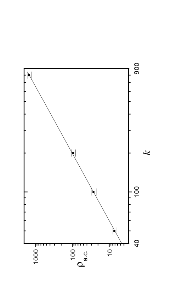
FIG. 6.: Log-Log plot of density of avoided crossings $\rho_{a.c}$ as a function of $k$ for gap sizes less than one quarter of the mean level spacing. $\rho_{a.c}$ scales as $k^{d}$ with $d=1.92\pm 0.1$.

FIG. 7.: Energy levels $E_{+}$, $E_{-}$ and $E_{0}$ as a function of $\ell/\ell_{int}$ for the $3-$levels hamiltonian analized in section III. The dotted lines indicates the asymptotes to $E_{-}$ and $E_{+}$. The distance $(E_{+}-E_{0})(0)={\sqrt{2}}\epsilon$ is also drawn.

REFERENCES

- [1] E. Vergini and M. Saraceno, Phys. Rev. E 52, 2204 (1995).
- [2] J. R. Nix and J. Sierk, Proc. Int. Conf. on Nuclear Physics, Bombay 1984 (World Scientific, Singapore, 1985), p. 365.
- [3] J. Blocki, Y. Boneh, J. R. Nix, J. Randrup, M. Robel, A. J. Sierk and W. J. Swiatecki, Ann. of Phys. 113, 330 (1978).
- [4] H. Hofmann, P. J. Siemens, Nuc. Phys. A 257, 1655 (1976); S. E. Koonin, R. L. Hatch and J. Randrup, Nuc. Phys. A 283, 87 (1977); S. E. Koonin and J. Randrup, Nuc. Phys. A 289, 475 (1977).
- [5] C. Yannouleas, M. Dworzecka and J. J. Griffin, Nuc. Phys. A 339, 219 (1980); C. Yannouleas, Nuc. Phys. A 439, 336 (1985).
- [6] W. Nörenberg, New Vistas in Nuclear Dynamics, ed. P. J. Brusserd and J. H. Kock (Plenumn Press, New York, 1986).
- [7] W. J. Swiatecki, Nuc. Phys. A 488, 375c (1988); J.Blocki, J. -J. Shi and W. J. Swiatecki, Nuc. Phys. A 554, 387 (1993).
- [8] C. Jarzynski, Phys. Rev. E 48, 4340 (1993).
- [9] Proceedings of the Les Houches Summer School of Theoretical Physics, Les Houches, 1981, edited by R. H. G. Helleman, G. Iooss and R. Stora (North-Holland, Amsterdam, 1983).
- [10] O. Bohigas, R. U. Haq and A. Pandey, in:Nuclear Data for Science and Technology, ed., K. H. Böckhff (Reidel, Dordrecht 1983) p. 809.
- [11] D. Hill and J. Wheeler, Phys. Rev. 89, 1102 (1952).
- [12] M. Wilkinson, J. Phys. A 21, 4021 (1988); M. Wilkinson, J. Phys. A 22, 2795 (1989).
- [13] A. Bulgac, G. Do Dang and D. Kusnezov, Ann. Phys. 242, 1 (1995); Phys. Rep. 264, 67 (1996).
- [14] L. D. Landau and E. M. Lifshitz, Quantum Mechanics, Vol.3 (Pergamon Press Ltd. Paris, 1958).
- [15] Mesoscopic Phenomena in Solids, edited by B. L. Altshuler, P. A. Lee and R. A. Webb (North-Holland, Amsterdam, 1991).
- [16] C. E. Zener, Proc. R. Soc. A 137, 696 (1932).
- [17] Diabatic basis have been used also in quantum chemistry to obtain a basis for which the coupling terms vanish (see for example F.T. Smith, Phys. Rev. 179, 111 (1969)).
- [18] D. Bohm, Quantum Theory, (Prentice-Hall, New York, 1951).
- [19] R. Balian and M. Veneroni, Ann. Phys. 135, 270 (1981).
- [20] L. A. Bunimovich, Commun. Math. Phys. 65, 295 (1979).
- [21] M. Wilkinson, Phys. Rev. A 41, 4645 (1990).
- [22] M. V. Berry, Ann. Phys. 131, 163 (1981).
- [23] E. J. Heller, in Wavepacket dynamics and Quantum Chaology, Proceedings of the Les Houches Summer School of Theoretical Physics, Les Houches, 1989, edited by M. J. Giannoni, A. Voros, and J. Zinn-Justin (North-Holland, Amsterdam, 1989).
- [24] H. P. Baltes and E. R. Hilf, Spectra of Finite Systems, (Bibliographisches Institut, Mannheim, 1976).
- [25] M. V. Berry and M. Tabor, J. Phys. A 10, 371 (1977).