Why air bubbles in water glow so easily

Abstract.

Sound driven gas bubbles in water can emit light pulses (sonoluminescence). Experiments show a strong dependence on the type of gas dissolved in water. Air is found to be one of the most friendly gases towards this phenomenon. Recently, ? have suggested a chemical mechanism to account for the strong dependence on the gas mixture: the dissociation of nitrogen at high temperatures and its subsequent chemical reactions to highly water soluble gases such as NO, NO₂, and/or NH₃. Here, we analyze the consequences of the theory and offer detailed comparison with the experimental data of Putterman’s UCLA group. We can quantitatively account for heretofore unexplained results. In particular, we understand why the argon percentage in air is so essential for the observation of stable SL.

1 Introduction

? discovered that a gas bubble levitated in water by a strong periodically modulated acoustic field can emit bursts of visible light so intense as to be observable to the naked eye, a phenomenon called single bubble sonoluminescence (SL). Previous workers had observed sonoluminescence in multibubble cavitation clouds: when a liquid is subjected to large negative pressures, the liquid rips apart into a cloud of bubbles, which then collapse violently. ? placed a photographic plate in the vicinity of a cavitating bubble cloud, and discovered that it was exposed to a low level of radiation. Single bubble SL is distinguished from multibubble sonoluminescene not only by the much higher light intensity, but also by the fact that the bubble remains in the oscillating state for billions of oscillation periods (days) without dissolving or changing its average size.

Soon after Gaitan’s initial discovery, Putterman’s research group at UCLA began to uncover a myriad of interesting dynamical properties of single bubble SL (?, ?, ?, ?, ?, ?, ?, ?, ?). The width of the light pulse is less than $50$ picoseconds. The accuracy of the flashes differs by less than $50$ picoseconds from cycle to cycle. The phenomenon shows strong dependence on the experimental parameters as the forcing pressure amplitude $P_{\rm a}$, the mass concentration $c_{\infty}$ of dissolved gas in the liquid far away from the bubble, and the temperature of the liquid. SL is only observed for $P_{\rm a}\sim 1.1$ atm – $1.5$ atm (for an ambient pressure of $P_{0}=1$ atm) for all gases. The dependence on $c_{\infty}$ is more subtle. For pure argon gas stable SL is observed only in a small window of extremely low concentration around $c^{\rm Ar}_{\infty}/c_{0}\sim 0.4\%$, whereas for air the water has to be degassed only down to $c^{\rm air}_{\infty}/c_{0}\sim 10-20\%$ to obtain stable SL. Here, $c_{0}$ is the saturation concentration of the gas in the liquid. Unstable SL, characterized by a “dancing bubble” and by oscillations in the phase and intensity of the light pulse, is observed in both cases (air and argon) for larger $c_{\infty}/c_{0}$. For pure nitrogen bubbles no stable SL is observed at all, only very weak unstable SL. Recently, ? also observed single bubble SL in nonaqueous fluids (alcohols) where the phenomenon shows a strong dependence on the type of liquid.

The major challenge in understanding the SL experiments is to determine how much of the phenomenology is hydrodynamic, how much is connected with the atomic properties of the gases, and how much stems from chemistry. To allow for detailed comparison between experiment and theory, ? calculated phase diagrams which depict domains of different bubble behaviors. They must depend on parameters which are easily experimentally adjustable. These are the forcing pressure $P_{\rm a}$ and the gas concentration $c_{\infty}$. As emphasized first by ? the ambient radius $R_{0}$ (i.e., the radius of the bubble under standard ambient conditions; $R_{0}\sim 5\mu{\rm m}$ in the SL experiments) is not an experimentally controllable parameter but adjusts itself dynamically.

We will see that much of above phenomenology can already be understood from the hydrodynamics and the stability of the bubble. Three types of instabilities will turn out to be important: (i) Shape instabilities of the bubble (?, ?, ?, ?, ?, ?), (ii) diffusional instabilities (?, ?, ?, ?), and (iii) chemical instabilities (?). ? consider only the instabilities (i) and (ii). They could quantitatively understand the experimental results (?, ?, ?) for pure argon bubbles, but not for gas mixtures with molecular constituents as e.g. air. For air the theoretical phase diagrams look very similar to those of argon, but experimentally (?, ?, ?) stable SL is found for about 100 times larger gas concentration, as already mentioned above. In this paper we elaborate our idea (?) that considering also chemical instabilities resolves this mystery.

2 Phase Diagrams for Sonoluminescence

To obtain phase diagrams of the bubble dynamics, one would have to solve the full three dimensional gas dynamical PDEs inside the bubble, coupled to the gas and fluid dynamics outside. This is numerically intractable; first, because the parameter space to be examined is huge, second, because a solution has to be computed for many millions of forcing cycles to cover the slow time scales of diffusional processes.

Consequently, we do need approximations to continue. The most successful approximation of bubble dynamics is the Rayleigh-Plesset (RP) equation for the radius $R(t)$ of the bubble as a function of time. This ODE was first written down by ?, while employed by the Royal Navy to investigate cavitation. Modern improvements have been made by ?, ?, ?, ?, and others. Recently, ? and ? were able to incorporate mass diffusion in the RP approach. This progress allowed us to study diffusional stability (?, ?).

The RP equation reads

$$R\ddot{R}+{3\over 2}\dot{R}^{2} = {1\over\rho_{\rm w}}\left(p(R,t)-P(t)-P_{0}\right)$$ (1)

$$+ {R\over\rho_{\rm w}c_{\rm w}}{{\rm d}\over{\rm d}t}\left(p(R,t)-P(t)\right)-4\nu{\dot{R}\over R}-{2\sigma\over\rho_{\rm w}R}$$

with the forcing pressure field

$$P(t)=P_{\rm a}\cos\omega t\enspace.$$ (2)

Parameter values for an argon bubble in water are the surface tension $\sigma=0.073{\rm kg}/{\rm s}^{2}$, water viscosity $\nu=10^{-6}{\rm m}^{2}/{\rm s}$, density $\rho_{\rm w}=1000{\rm kg}/{\rm m}^{3}$, and speed of sound $c_{\rm w}=1481{\rm m}/{\rm s}$. The driving frequency of the acoustic field is $\omega/2\pi=26.5{\rm kHz}$ and the external pressure $P_{0}=1$ atm. We assume that the pressure inside the bubble varies according to the van der Waals law

$$p(R(t))=\left({R_{0}^{3}-h^{3}\over R^{3}(t)-h^{3}}\right)^{\kappa}\enspace,$$ (3)

where $h=R_{0}/8.86$ is the hard core van der Waals radius. The effective polytropic exponent is taken to be $\kappa=1$ (?) for the small bubbles employed here.

Fig. 1.: (a) Forcing pressure $P(t)=P_{\rm a}\cos\omega t$, $P_{\rm a}=1.3$ atm for two cycles and the corresponding (b) bubble radius $R(t)$ and (c) bubble ambient radius $R_{0}(t)$. The bubble is near an equilibrium state. The gas concentration is $c^{\rm Ar}_{\infty}/c_{0}=0.004$. The ambient radius shown here results from the numerical solution of the convection-diffusion PDEs, for details we refer to ?.

In figure 1 we plot $R(t)$ resulting from (1), together with the forcing pressure $P(t)$. The radius shows a characteristic collapse which can be very violent for large forcing $P_{\rm a}$. It is right at this collapse when the light pulse is emitted. ? and ? have shown that the experimental curves of the radius look very similar to that of figure 1 and that (1) can be used to fit the dynamics of the radius. There may be small quantitative discrepancies with the real dynamics, but they are clearly in the range of the experimental error.

First, we address the question of shape instabilities , i.e., non-spherical deformations of the gas-water interface. There are basically two different types of shape instabilities, distinguished by the time scale over which they act. Parametric instabilities act over many bubble oscillation periods, and are the result of accumulation of small perturbations. Rayleigh-Taylor instabilities occur when a light fluid is accelerated into a heavy fluid. Here, they happen during a short time directly after the bubble collapse. Although the process is very rapid ($\sim 10^{-9}$ s), detailed calculations (?, ?) show that at high forcing, a perturbation of a few Å can grow to be as large as the bubble during this time. The differing time scales over which these instabilities act have consequences for the final state of the bubble: after a Rayleigh-Taylor instability, bubbles are typically destroyed, whereas after a parametric instability, the bubble can remain trapped in the acoustic field. Figure 2 shows the borderline between stability and instability in the ambient radius $R_{0}$ vs forcing amplitude $P_{\rm a}$ parameter space. The diagram is calculated for an argon bubble in water (?). Also depicted in figure 2 is the threshold curve beyond which the bubble wall speed exceeds the speed of sound. We take this as a condition for the development of shock waves in the bubble. Following the common assumption that shocks are necessary for sonoluminescence to occur (?, ?, ?), we thus get a further restriction for the parameter range of sonoluminescing bubbles.

Fig. 2.: Parametric instability (solid), Rayleigh-Taylor instability (dashed), and shock condition (Mach=1, long dashed). SL is only possible in a small regime of large $P_{\rm a}\sim 1.3$ atm and small $R_{0}\sim 3\mu{\rm m}$ where the bubble is spherically stable and the shock condition is fulfilled. Also shown are the diffusive equilibria for $c^{\rm Ar}_{\infty}/c_{0}=0.5$, $0.02$, and $0.002$. Whenever the slope is positive, the diffusive equilibrium is stable. At $P_{a}=1.3$atm diffusively stable SL bubbles are only possible for very low concentration $c^{\rm Ar}_{\infty}/c_{0}\sim 0.002-0.004$. For larger $P_{a}$ even lower concentrations are required.

Let us now turn to diffusive stability. Measurements of the time between successive light flashes show that the total mass of the bubble can remain constant to high accuracy (?, ?, ?, ?) for days, if the gas concentration is in an appropriate regime. This result contradicts classical notions about the dynamics of periodically forced bubbles: An unforced bubble of ambient radius $R_{0}$ dissolves over a diffusive time scale, $\tau\sim\frac{\rho_{0}R_{0}^{2}}{D(c_{0}-c_{\infty})}$ (?), where $\rho_{0}$ is the ambient gas mass density in the bubble and $D$ is the diffusion constant of the gas in the liquid. On the other hand, a strongly forced bubble grows by rectified diffusion, as first discovered by ? and later explored by ?, ?, ?. This is because at large bubble radius the gas pressure in the bubble is small, resulting in a mass flux into the bubble; conversely, when the bubble radius is small there is a strong mass outflux. Both processes can be observed in figure 1c which shows the ambient radius $R_{0}(t)$ corresponding to the actual bubble radius $R(t)$ of figure 1b. Since the diffusive time scale is much larger than the short time the bubble spends at small radii, gas cannot escape from the bubble during compression; the net effect is bubble growth. At a special value $R_{0}^{\rm e}$ of the ambient radius rectified diffusion and normal diffusion balance. The main result of ? was that contrary to above intuition the equilibrium points $R_{0}^{\rm e}$ can be stable. ? showed that for argon bubbles the window of stability in $c^{\rm Ar}_{\infty}/c_{0}$ is in quantitative agreement with experiment.

Fig. 3.: Phase diagram in the $c^{\rm Ar}_{\infty}/c_{0}$ vs $P_{\rm a}/P_{0}$ parameter space. For the SL phase we assumed that the light production mechanism works beyond the Mach=1 curve. Bubbles at very large $P_{\rm a}$ may be Rayleigh-Taylor unstable.

Fig. 4.: (a) The phase of light emission $\phi_{\rm s}(t)$ (upper) and the corresponding ambient radius $R_{0}(t)$ (lower) for $P_{\rm a}=1.3$ atm for three different gas concentrations $c^{\rm Ar}_{\infty}/c_{0}=0.004$, $c^{\rm Ar}_{\infty}/c_{0}=0.066$, and $c^{\rm Ar}_{\infty}/c_{0}=0.26$, corresponding to a gas pressure of $3$ mmHg, $50$ mmHg, and $200$ mmHg, respectively. The strength of the micro-bubble pinch-off at $R_{0}=5\mu m$, i.e. the decrease of the ambient radius, is picked randomly. The concentration values are chosen as in the experiment of ? which is shown in (b), copied from Fig. 4 of that reference. That figure also shows the relative phase of light emission for air bubbles: Stable SL is achieved at much higher concentration $c^{\rm air}_{\infty}/c_{0}=0.2$, corresponding to a gas pressure of 150 mmHg. It is this discrepancy between argon (or other inert gases) and air which we resolve in this paper.

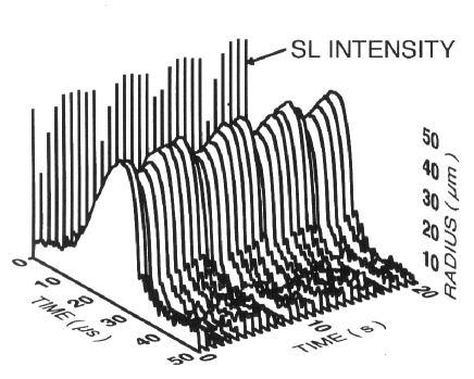
Fig. 5.: This figure is reproduced from figure 6 of ?. It shows the SL intensity and bubble radius as a function of time for a nitrogen bubble with $5\%$ argon. The drive level $P_{\rm a}$ is near the upper threshold of SL. The gas is dissolved at $150$ mmHg, i.e. $c^{\rm mix}_{\infty}/c_{0}\approx 20\%$. The bubble radius exhibits the characteristic pattern of growth and microbubble pinch-off of unstable SL.

Figure 3 shows the total phase diagram as a function of $c^{\rm Ar}_{\infty}/c_{0}$ and $P_{\rm a}/P_{0}$. Three different states are possible: The label stable SL denotes the region of parameter space where the bubble can be diffusively stable and also stable to shape oscillations. In the region no SL the bubble dissolves, while in the unstable SL domain the bubble is not in diffusive equilibrium but can nonetheless survive. That this is possible is quite nontrivial, and was first shown by experiments of ? and ?.

In the unstable SL phase the bubble is growing by rectified diffusion until it hits the parametric instability. The bubble becomes shape unstable and microbubbles pinch off. If the remaining bubble is still large enough, the process begins again. Figure 4a shows the ambient radius $R_{0}$ and the corresponding phase $\phi_{\rm s}$ of the light emission relative to the forcing field as a function of time as calculated from our theoretical Rayleigh-Plesset approach (?). We chose the same three gas concentrations as in the experiment of ? which we present in Fig. 4b for comparison. Both in our calculations and in experiment we are in the unstable SL regime for the two larger argon partial pressures (200 mmHg and 50 mmHg), whereas the lowest value of 3 mmHg is in the stable SL regime, again both in theory and experiment. Argon bubbles thus seem to be well understood.

Another experimental result (now for a gas mixture) in the unstable SL regime is shown in Fig. 5. We observe the maximal radius $R_{\rm max}$ and the light intensity growing on the diffusional time scale $\sim 1{\rm s}$ until the bubble hits the parametric instability and the process starts over. Note that our interpretation of the unstable SL regime also accounts for the observed “dancing” of the bubble: the pinch-off of the microbubbles leads to recoils of the bubble. The dancing frequency should be the higher the larger $c^{\rm Ar}_{\infty}$ is.

Although the above results for pure argon bubbles are in excellent agreement with experiments, we still have above mentioned severe discrepancy for air bubbles and other gas mixtures that stable SL is observed for much larger concentrations than expected from our phase diagram Fig. 3. E.g., in air we have stable SL for $c^{\rm air}_{\infty}/c_{0}\approx 0.1-0.2$, depending on the forcing pressure. This discrepancy was first pointed out in the qualitative arguments of ? who found that air bubbles in the range where stability is observed should be unstable from a theoretical point of view, based on RP dynamics. The reason for this can be seen in the phase diagram above: if the diagram is repeated for air instead of argon, the stable equilibria still occur at very low concentrations, namely $c^{\rm air}_{\infty}/c_{0}\approx 0.004.$ Based on this discrepancy, Löfstedt et al. hypothesize an “as yet unidentified mass ejection mechanism.”

3 A Chemical Resolution of the Paradox

In joint work with Todd F. Dupont and Blaine Johnston of the University of Chicago (?), we have pointed out that this paradox can be resolved by considering chemical instabilities. Namely, it is well known that the temperature in the bubble becomes very high after the collapse. Fits of the spectra of emitted radiation to a black body law give effective temperatures of up to $25000{\rm K}$ (?). This temperature exceeds the dissociation temperature for nitrogen gas ($\sim 9000{\rm K}$) as well as for all other molecular constituents of air. The nitrogen, oxygen, and hydrogen radicals will recombine to finally form NO, NO₂, and/or NH₃. All of these gases are highly soluble in water, forming nitric and nitrous acid and NH₄OH. The consequence is that the bubble is finally depleted from the molecular constituents of air.

Even beyond “burning” of all initial nitrogen in the bubble we expect that whenever the bubble is large it will still suck gas from the water into the bubble which will also be “burnt” during the next compression cycle. The bubble thus constitutes a reaction chamber for the dissolved molecular gas. The reaction products should be detectable. ? estimated a production rate of $\sim 10^{11}{\rm mol}/{\rm s}$ per container volume ($\sim 1{\rm l}$). Let us assume that the main product is NH₄OH. Starting with the optimal pH=7 we should thus get a doubling of OH^- ions within about three hours and a pH change up to pH=8 (i.e., $c_{\rm{OH}^{-}}=10^{-6}{\rm mol}/{\rm l}$) in about a day of running the experiment. Many other ways of detection rather than simply measuring the pH seem possible. An ion chromatographer will give a detailed answer on what ions are produced.

For the present paper we only need the assumption that even when air was initially dissolved in water, a sonoluminescing bubble essentially consists of inert gases as these are the only gases which do not react with water at the high temperatures achieved in single bubble SL; they are simply recollected by the expanding bubble as seen in Fig. 1c.

The dissociation hypothesis suggests that for gas mixtures the relevant concentration quantity is still the argon concentration $c_{\infty}^{\rm Ar}/c_{0}$ which now is

$${c_{\infty}^{\rm Ar}\over c_{0}}=q\cdot\frac{c_{\infty}^{\rm mix}}{c_{0}}\enspace,$$ (4)

where $q$ is the percentage of argon in the mixture. For air we have $q=0.01=1\%$. Here we have neglected the differences in solubility $c_{0}$ of the different gases. This difference enters in two counteracting ways: first, (4) must be corrected by the ratio $c_{0}^{\rm Ar}/c_{0}^{{\rm N}_{2}}$ of the solubilities between argon and nitrogen, which is about three. But second, because of the different solubilities the percentage of argon in dissolved air will not be the usual $1\%$, but will be larger. Possibly, this percentage even depends on the degree of degassing of the water. These two effects will probably roughly compensate each other and we decided to disregard them for the time being.

In the following section we discuss how the dissociation hypothesis can explain the experimental UCLA results on gas mixtures (?, ?, ?, ?). We point out that our detailed unpublished investigations of mixtures of gases demonstrate that it is impossible to understand these discrepancies within diffusive theories alone, i.e., by disregarding chemical reactions.

Fig. 6.: Transition towards the SL regime for argon bubbles (a) and for air bubbles (b). Only for air bubbles a breakdown in the radius is seen near the onset of SL, signaling the threshold for nitrogen dissociation. Figure (a) is a reproduction from figure 4 from ?, the total gas concentration is about 150 mmHg. This means $c^{\rm air}_{\infty}/c_{0}=0.2$ in the unstable SL regime in agreement with the observations. Figure (b) is a reproduction from figure 2 of ?. The gas saturation is about $10\%$, corresponding to $c^{\rm Ar}_{\infty}/c_{0}=0.01\cdot 0.1=0.001$. According to Fig. 3 we have stable SL around $P_{\rm a}\sim 1.4$ atm which again is in rough agreement with experiment.

4 Comparison with the UCLA Experiments

Where to expect stable SL in air bubbles? From our phase diagram Fig. 3 we know that for $P_{\rm a}=1.3$ atm stable SL is found in a small window of $c^{\rm Ar}_{\infty}/c_{0}\sim 0.3-0.4\%$ for pure argon gas. Equation (4) thus gives $c^{\rm air}_{\infty}/c_{0}\sim 30-40\%$ for air dissolved in water. The experimental values seem to be slightly smaller, but clearly within the error range of both our assumptions and the measurements.

The transition towards SL with increasing forcing pressure $P_{\rm a}$ is shown in Fig. 6 for both argon and air bubbles. For pure argon bubbles the transition to SL is very smooth. For air, however, one can observe a breakdown of the bubble radius at about $1.1$ atm, signaling that the dissociation threshold of N₂ is achieved. Before the transition the bubble is filled with a mixture of nitrogen, oxygen, and argon, and the ambient radius is determined by the combination of all three gases. After the dissociation threshold, only argon is left in the bubble.

We now also see why stable SL is so easily obtained in air bubbles: The window of stability is larger compared to argon bubbles and the water has to be degassed much less. But even more friendly conditions are possible: Our theory suggests that it should be possible to obtain stable SL without degassing, namely by choosing the percentage $q$ of argon so that the window of stable SL is around $c^{\rm mix}_{\infty}/c_{0}\sim 100\%$. With $q\sim 0.35\%$ we obtain as window of stable SL $c^{\rm mix}_{\infty}/c_{0}\sim 85-115\%$.

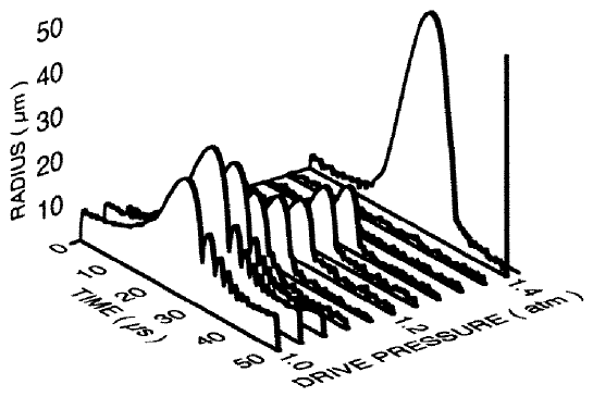
Fig. 7.: This figure is reproduced from figure 11 of ?. It shows the transition to SL for a bubble filled with an initial $0.1\%$ xenon in nitrogen gas mixture at a partial pressure of 150 mmHg. According to our dissociation hypothesis this corresponds to $c^{\rm Xe}_{\infty}/c_{0}=0.0002$ for a pure sonoluminescing xenon bubble. From our phase diagram Fig. 3 which is (with tiny corrections) also valid for xenon we conclude that bubbles driven at $P_{\rm a}=1.3$ atm dissolve for these low concentrations, whereas bubbles at $P_{\rm a}=1.4$ atm show stable SL, just as seen in this experimental figure.

For even lower concentration $q<0.3\%$ (at $P_{\rm a}=1.3$ atm) no stable SL regime is left for $c_{\infty}^{\rm mix}/c_{0}<100\%$. The experiment of ? with $q=0.1\%$ xenon in nitrogen at $c_{\infty}^{\rm mix}/c_{0}=0.2$ shown in Fig. 7 relates to exactly that situation. ? find a range of forcing pressures $P_{\rm a}\approx 1.3-1.4$ atm where stable bubbles cannot be seeded. Above $1.4$ atm, stable SL exists, and below $1.3$ atm there are non–sonoluminescing bubbles. The reason for this “gap” is that at these high forcing pressures all nitrogen is dissociated and the bubble only contains the inert gas xenon. Then, according to our phase diagram Fig. 3 (which also holds for xenon), at $P_{\rm a}=1.3$ atm the xenon concentration $c_{\infty}^{\rm Xe}=q\cdot c^{\rm mix}_{\infty}/c_{0}=0.001\cdot 0.2=0.0002$ is in the no SL regime and bubbles dissolve. But at higher forcing pressure $P_{\rm a}\sim 1.4$ atm we can again enter the stable SL regime for that concentration, see Fig. 3: a pure xenon bubble can emit light and acts as a chemical reaction chamber, transferring the dissolved nitrogen to its high temperature reaction products.

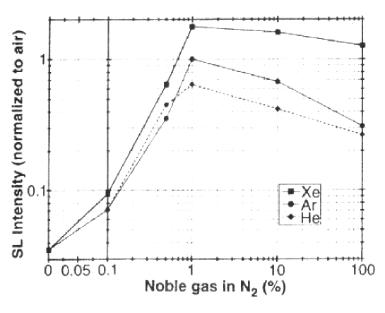
Fig. 8.: This figure is reproduced from figure 1 of ?. It shows the SL intensity from a SL bubble in water as a function of the percentage (mole fraction) of noble gas mixed with nitrogen. The gas mixture was dissolved in water at a pressure head of 150 mmHg, i.e., $c_{\infty}^{\rm mix}/c_{0}\sim 0.2$.

The transition from the no SL regime in Fig. 3 to the SL regime can also be seen in Fig. 8, where the SL light intensity is plotted as a function of $q$ for fixed $P_{\rm a}$ (we assume $P_{\rm a}=1.3$ atm) and fixed $c^{\rm mix}_{\infty}/c_{0}\sim 0.20$. According to our theory the transition for $c_{\infty}^{\rm Ar}/c_{0}=0.003$ should occur at $q=(c_{\infty}^{\rm Ar}/c_{0})/(c^{\rm mix}_{\infty}/c_{0})=1.5\%$ in pretty good agreement with Fig. 8 where we indeed observe that strong SL is “switched on” at about that concentration. Our theory also predicts that near the switch on we always have stable SL, whereas for larger $q$ unstable SL develops. Here we expect unstable SL for $q>2\%$, a prediction which should be verified.

An example for unstable SL was already shown in Fig. 5. Indeed, for that figure we have $q=5\%$. Thus, from (4) we have $c_{\infty}^{\rm Ar}/c_{0}=0.05\cdot 0.2=0.01$ and according to our phase diagram Fig. 3 and equation (4) we are well in the unstable SL regime, just in agreement with the observations.

Next, we consider the case of a pure nitrogen bubble. Below the dissociation threshold it is “jiggling”, i.e. growing by rectified diffusion and shedding microbubbles. Above the threshold, the nitrogen is taken away, so the bubble will necessarily dissolve. Indeed, ? show that pure nitrogen bubbles dissolve in a matter of seconds. In figure 5 of their work it is demonstrated that pure nitrogen bubbles show “periodic” oscillations in their light intensity. We do not understand what sets the oscillation period, though we speculate that it is connected to the dissociation of nitrogen in the bubble, as well as the unstable “jiggling” of the bubble. Perhaps by understanding the origin of these oscillations one could deduce the temperature inside the bubble.

Another experiment supports our dissociation hypothesis. ? analyze SL in $\rm{H}_{2}$ and $\rm{D}_{2}$ gas bubbles, both in normal and in heavy water. One would expect that the SL intensity curves would group according to the gas content as it is the gas dynamics inside the bubble which determines the strength of the light emission. However the four (H₂ in H₂O, H₂ in D₂O, D₂ in H₂O, and D₂ in D₂O) experiments group according to the surrounding liquids. This suggests the following scenario: Both the gas and the liquid vapor in the bubble dissociate during the (hot) compression phase and recombine later on during expansion. As much more liquid than gas is around, recombination will yield gases primarily composed of the constituents of the liquid vapor. E.g., in the experiment using $\rm{H}_{2}$ in $\rm{D}_{2}\rm{O}$, the $\rm{H}_{2}$ will shortly be replaced by $\rm{D}_{2}$ formed from the heavy water, whereas the amount of $\rm{H}_{2}\rm{O}$ formed from $\rm{H}_{2}$ will be negligible. Thus the density of the bubbles in D₂O will eventually be larger by a factor of two compared to the density of bubbles in H₂O. Following our recently proposed laser theory of SL (with R. Rosales, (?)), it is this density difference which may be the origin of the considerably different SL intensities observed in normal and heavy water by ?.

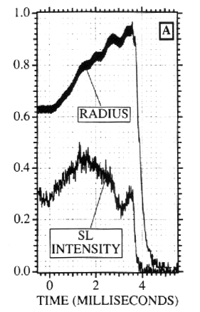
Fig. 9.: This figure is reproduced from figure 4 of ?. It shows the dynamic response of the radius and the intensity of SL to a sudden change in the drive level $P_{\rm a}$. The bubble is boosted into the unstable SL regime where it finally becomes shape unstable and bursts.

There is one final experimental figure which we want to discuss here. It is Fig. 9, showing the maximal radius $R_{\rm max}(t)={\rm max}\{R(t^{\prime})|t\leq t^{\prime}\leq t+T\}$ and the intensity as a function of time when the forcing pressure $P_{\rm a}$ is suddenly strongly increased. On this increase, the bubble is pushed in the unstable SL domain and starts to grow rapidly thanks to rectified diffusion. But why is the growth rate of $R_{\rm max}$ so wiggly whereas the growth rate of the ambient radius does not show these wiggles, as seen from Fig. 4?

Fig. 10.: The maximal bubble radius $R_{\rm max}$ as a function of the ambient radius $R_{0}$ for two forcing pressures $P_{\rm a}=1.1$ atm and 1.2atm. It shows characteristic wiggles. The dashed lines depict the $R_{\rm max}\propto R_{0}^{3/5}$ scaling law.

The answer is that $R_{\rm max}$ itself shows wiggles as a function of the ambient radius, as observed in ? and analyzed in detail by ?. In figure 10 we present $R_{\rm max}(R_{0})$, whose wiggles are probed in figure 9 by the growing $R_{0}$. The averaged scaling law is given by $R_{\rm max}\propto R_{0}^{3/5}$ (?).

In diffusionally stable regimes these wiggles may lead to multiple stable equilibria, as suggested in ? and possibly observed by ?. ? pointed out that the origin of the wiggles and the resulting multiple equilibria are resonances in the RP dynamics.

5 Conclusions

This paper has summarized our current understanding of the bubble dynamics leading to single bubble sonoluminescence. Our central theoretical result is the phase diagram of SL figure 3 from ?. It can only be calculated in the Rayleigh-Plesset SL bubble approach including both shape oscillations and diffusion. The phase diagram allows to quantify the differences between argon and air bubbles found by ?, guiding them to suggest a “yet unidentified mass ejection mechanism” for air bubbles. We now believe that this mechanism is chemical, namely the dissociation of gas molecules in highly forced gas bubbles and their subsequent reactions. As pointed out in this paper, with this “nitrogen–dissociation hypothesis” many experimental results can be explained. To further verify this hypothesis, experiments should search for the various reaction products.

One issue that we have barely touched in this paper is the mechanism for the light emission. The traditional theory is that shocks are emitted from the bubble wall, and heat up the gas in the bubble to such an extent that light emission is induced. Experimentally there are strong dependences of the light intensity on liquid, gas and forcing pressure. These cannot be explained within the context of simple bubble dynamics presented here, and also do not seem to be understandable within the shock theory. The shock theory relies on a singular solution to the hydrodynamic equations; singularities are typically of universal character and very insensitive to external conditions. However, the fact that experiments on single bubble SL demonstrate such sensitivity to parameters contradicts this principle. The most dramatic example of this is the initial observation of single bubble SL by ?: it caused great excitement because the light intensity is so much higher than in multibubble SL. However, the shock theory should apply equally well to both cases. These ideas suggest that the shock theory has intrinsic shortcomings. To overcome these problems ? recently proposed a “hydrodynamic laser” theory for SL bubbles. It stipulates that the bubble can accumulate acoustic energy inside the bubble which acts as a kind of acoustic resonator.

We hope that our present and ongoing work will help to answer one of the essential remaining questions on SL: How hot does the gas become in the center of the bubble? Our hope is that the presence of intermediate or final chemical reaction products can be thought of as a thermometer. – The perspectives are appealing: A tiny air bubble in water is used as a chemical reaction chamber and a micro-laboratory for high temperature chemistry!

Acknowledgements:
We thank our colleagues and collaborators B. Barber, L. Crum, K. Drese, T. F. Dupont, B. Gompf, S. Grossmann, B. Johnston, L. Kadanoff, W. Kang, D. Oxtoby, Th. Peter, S. Putterman, R. Rosales and J. Young for many useful and thought provoking discussions and suggestions. This research was supported by the DFG through its SFB185. MB acknowledges an NSF postdoctoral fellowship.

References

- 1 bar91Barber and Putterman (1991) Barber, B.P., and Putterman, S.J., “Observation of synchronous picosecond sonoluminescence”, Nature (London) 352, 318-320 (1991); “Ligth scattering measurements of the repetitive supersonic implosion of a sonoluminescing bubble”, Phys. Rev. Lett. 69, 3839-3842 (1992).
- 2 bar94Barber et al. (1994) Barber, B.P., Wu, C. C., Löfstedt, R., Roberts, P. H., and Putterman, S. J., “Sensitivity of sonoluminescence to experimental parameters” Phys. Rev. Lett. 72, 1380-1383 (1994).
- 3 bar95Barber et al. (1995) Barber, B.P., Weninger, K., Löfstedt, R., and Putterman, S.J., “Observation of a new phase of sonoluminescence at low partial pressures”, Phys. Rev. Lett. 74, 5276-5279 (1995).
- 4 bla49Blake (1949) Blake, F.G., Harvard University Acoustic Research Laboratory Technical Memorandum 12, 1 (1949).
- 5 bre95Brenner, Lohse, and Dupont (1995) Brenner, M. P., Lohse, D., and Dupont, T. F., “Bubble shape oscillations and the onset of sonoluminescence”, Phys. Rev. Lett. 75, 954-957 (1995).
- 6 bre96Brenner et al. (1996a) Brenner, M.P., Lohse, D., Oxtoby, D., and Dupont, T.F., “Mechanisms for stable single bubble sonoluminescence”, Phys. Rev. Lett. 76, 1158-1161 (1996).
- 7 bre96dBrenner et al. (1996b) Brenner, M.P., Rosales, R. R., Hilgenfeldt, S., and Lohse, D., “Acoustic energy storage in single bubble sonoluminescence”, preprint, submitted to Phys. Rev. Lett., April 1996.
- 8 cru80Crum (1980) Crum, L.A., “Measurements of growth of air bubbles by rectified diffusion”, J. Acoust. Soc. Am. 68, 203-211 (1980).
- 9 cru94bCrum and Cordry (1994) Crum, L.A., and Cordry, S., “Single bubble sonoluminescence”, in Bubble dynamics and interface phenomena, edited by J.Blake etal (Kluwer Academic Publishers, Dordrecht, 1994), p. 287-297.
- 10 ell69Eller (1969) Eller, A., “Growth of bubbles by rectified diffusion”, J. Acoust. Soc. Am. 46, 1246-1250 (1969).
- 11 ell70Eller and Crum (1970) Eller, A., and Crum, L.A., “Instability of the motion of a pulsating bubble in a sound field”, J. Acoust. Soc. Am. Suppl. 47, 762-767 (1970).
- 12 eps50Epstein and Plesset (1950) Epstein, P.S., and Plesset, M.S., “On the stability of gas bubbles in liquid-gas solutions”, J. Chem. Phys. 18, 1505-1509 (1950).
- 13 fre34Frenzel and Schultes (1934) Frenzel, H., and Schultes, H., Z. Phys. Chem. 27B, 421 (1934).
- 14 fyr94Fyrillas and Szeri (1994) Fyrillas, M.M., and Szeri, A.J., “Dissolution or growth of soluble spherical oscillating bubbles”, J. Fluid Mech. 277, 381-407 (1994).
- 15 gai90Gaitan et al. (1990) Gaitan, D.F., “An experimental investigation of acoustic cacitation in gaseous liquids”, Ph.D. thesis, The University of Mississippi, 1990; Gaitan, D.F., Crum, L.A., Roy, R.A., and Church, C.C., Sonoluminescence and bubble dynamics for a single bubble, stable cavitation bubble”, J. Acoust. Soc. Am. 91, 3166-3183 (1992).
- 16 gre93Greenspan and Nadim (1993) Greenspan, H.P., and Nadim, A., “On sonoluminescence of an oscillating gas bubble”, Phys. Fluids A 5, 1065-1067 (1993).
- 17 bre96cGrossmann et al. (1996) Grossmann, S., Hilgenfeldt, S., Lohse, D., and Brenner, M.P., “Analysis of the Rayleigh-Plesset bubble dynamics for large forcing pressure”, in preparation, May 1996.
- 18 hil96Hilgenfeldt, Lohse, and Brenner (1996) Hilgenfeldt, S., Lohse, D., and Brenner, M.P., “Phase diagrams for sonoluminescing bubbles”, preprint, Phys. Fluids, November 1996.
- 19 hil92Hiller, Putterman, and Barber (1992) Hiller, R., Putterman, S.J., and Barber, B.P., “Spectrum of synchronous picosecond sonoluminescence”, Phys. Rev. Lett. 69, 1182-1185 (1992).
- 20 hil94Hiller et al. (1994) Hiller, R., Weninger, K., Putterman, S.J., and Barber, B.P., “Effect of noble gas doping in single bubble sonoluminescence”, Science 266, 248-234 (1994).
- 21 hil95Hiller and Putterman (1995) Hiller, R., and Putterman, S.J., “Observation of isotope effects in sonoluminescence” Phys. Rev. Lett. 75, 3549-3551 (1995).
- 22 lau76Lauterborn (1976) Lauterborn, W., “Numerical investigation of nonlinear oscillations of gas bubbles in liquid”, J. Acoust. Soc. Am. 59, 283-293 (1976).
- 23 loh96Lohse et al. (1996) Lohse, D., Brenner, M.P., Dupont, T., Hilgenfeldt, S., and Johnston, B., “Sonoluminescence: Air bubbles as chemical reaction chambers”, preprint, April 1996.
- 24 loe93Löfstedt, Barber, and Putterman (1993) Löfstedt, R., Barber, B.P., and Putterman, S.J., “Toward a hydrodynamic theory of sonoluminescence”, Phys. Fluids A 5, 2911-2928 (1993).
- 25 loe95Löfstedt et al. (1995) Löfstedt, R., Weninger, K., Putterman, S.J., and Barber, “Sonoluminescing bubbles and mass diffusion” B.P., Phys. Rev. E 51, 4400-4410 (1995).
- 26 mos94Moss et al. (1994) Moss, W., Clarke, D., White, J., and Young, D., “Hydrodynamic simulations of bubble collapse and picosecond sonoluminescence”, Phys. Fluids 6, 2979-2985 (1994).
- 27 ple49Plesset (1949) Plesset, M., “The dynamics of cavitation bubbles”, J. Appl. Mech. 16, 277 (1949).
- 28 ple54Plesset (1954) Plesset, M., “On the stability of fluid flows with spherical symmetry”, J. Appl. Phys. 25, 96-98 (1954).
- 29 ple77Plesset and Prosperetti (1977) Plesset, M. and Prosperetti, A., “Bubble dynamics and cavitation” Ann. Rev. Fluid Mech. 9, 145-185 (1977).
- 30 pro77Prosperetti (1977) Prosperetti, A., “Viscous effects on perturbed spherical flows”, Quart. Appl. Math. 34, 339-352 (1977).
- 31 ray17Lord Rayleigh (1917) Rayleigh, Lord, “On the pressure developed in a liquid on the collapse of a spherical bubble”, Philos. Mag. 34, 94 (1917).
- 32 str71Strube (1971) Strube, H.W., “Numerische Untersuchungen zur Stabilität nichtsphärisch schwingender Blasen”, Acustica 25, 289-303 (1971).
- 33 wen95Weninger et al. (1995) Weninger, K., Hiller, R. Barber, B., Lacoste, D., and Putterman, S., “Sonoluminescence from single bubbles in non-aqueous liquids: new parameter space for sonochemistry”, J. Phys. Chem. 99, 14195 (1995).
- 34 wu93Wu and Roberts (1993) Wu, C.C., and Roberts, P.H., “Shock-wave propagation in a sonoluminescing gas bubble”, Phys. Rev. Lett. 70, 3424-3427 (1993); “A model of sonoluminescence”, Proc. R. Soc. London A 445, 323-349 (1994).