Three-dimensional spontaneous magnetic reconnection in neutral current sheets

Abstract

Magnetic reconnection in an antiparallel uniform Harris current sheet equilibrium, which is initially perturbed by a region of enhanced resistivity limited in all three dimensions, is investigated through compressible magnetohydrodynamic simulations. Variable resistivity, coupled to the dynamics of the plasma by an electron-ion drift velocity criterion, is used during the evolution. A phase of magnetic reconnection amplifying with time and leading to eruptive energy release is triggered only if the initial perturbation is strongly elongated in the direction of current flow or if the threshold for the onset of anomalous resistivity is significantly lower than in the corresponding two-dimensional case. A Petschek-like configuration is then built up for $\sim 10^{2}$ Alfvén times, but remains localized in the third dimension. Subsequently, a change of topology to an O-line at the center of the system (“secondary tearing”) occurs. This leads to enhanced and time-variable reconnection, to a second pair of outflow jets directed along the O-line, and to expansion of the reconnection process into the third dimension. High parallel current density components are created mainly near the region of enhanced resistivity.

Phys. Plasmas, Vol. 7, No. 1, January 2000 issue

I INTRODUCTION

The reconnection of magnetic field lines is one of the fundamental processes that lead to the eruptive release of stored magnetic energy in plasmas. A large number of observations and experiments, e.g., solar flares,[1, 2] geomagnetic substorms,[3] the sawtooth instability in fusion experiments,[4] and laboratory reconnection experiments,[5, 6] support this hypothesis. Magnetic reconnection is important for the evolution of magnetohydrodynamic (MHD) instabilities (e.g., the tearing mode[7] and magnetic island coalescence[8, 9, 10]) in current sheets which are generally involved in the energy release process. It is also important at the dissipative scales in MHD turbulence.[11, 12] To explain the short time scales of the energy release processes in spite of large values of the Lundquist number $S=\mu_{0}LV_{A}/\eta_{0}$, fast reconnection models have been proposed but are generally restricted to two-dimensional geometry, including the stationary Petschek model[13] and the spontaneous fast reconnection model.[14] Both these models are one-fluid descriptions in which resistivity provides the nonideal effect required for reconnection and in both models the resistivity is localized at the central magnetic X-point.

Models distinguishing between electron and ion effects, such as Hall MHD,[15, 16] two-fluid MHD,[17] or kinetic treatments,[18, 19] permit still higher reconnection rates, even in the absence of resistivity. However, all these models require significant computational effort, which still prevents following the evolution of microscopic perturbations to large spatial and temporal scales in three dimensions.

In the spontaneous fast reconnection model, a current sheet equilibrium is initially perturbed by a localized region of enhanced (anomalous) resistivity in the sheet center, which leads to the development of a simple X-point structure. Anomalous resistivity is permitted to occur in this model also at later times of the evolution if a threshold of the local current density ${\bf j}$ or of the local electron-ion drift velocity ${\bf v}_{D}=(m_{i}/e)\,{\bf j}/\rho$ is exceeded ($m_{i}$ – ion mass, $e$ – elementary charge, $\rho$ – mass density). This couples the reconnection-driven flow to the evolution of the resistivity and enables a positive feedback that amplifies the dynamics in the reconnection region. This mechanism is of particular interest for eruptive energy release events since it involves a threshold for onset, is initially self-amplifying, and is fast, i.e., it leads to rates of magnetic flux change at the magnetic null point (reconnection rates) higher than the Sweet-Parker rate[20, 21] and to Alfvénic outflows.

Several basic 3D effects of magnetic reconnection have already been analyzed in simulations using temporarily or spatially constant resistivity such as the diversion of current flow by the reconnection-driven outflow,[22, 23, 24, 25] the creation of interlinked magnetic flux tubes by multiple areas of enhanced resistivity,[26] and the tunneling of magnetic flux tubes.[27] The very question of the formation and maintenance of the spontaneous fast reconnection process in a three-dimensional system with dynamically coupled resistivity has only recently been investigated by Ugai and Shimizu.[28] The latter authors generalized the 2D model by introducing a three-dimensional initial perturbation by anomalous resistivity $\eta_{an}(x,y,z,t)$ in a triple current sheet geometry with antiparallel magnetic field, ${\bf{B}}=B(y)\,{\bf{e}}_{x}$. By varying the $z$ extension of the initial perturbation, they found that the spontaneous fast reconnection process occurs also in 3D but only if the region of perturbation is strongly anisotropic, extending in the $z$ direction by at least 4 current sheet widths.

Such an anisotropy with preferred elongation across the magnetic field cannot be expected to occur spontaneously without additional assumptions. In magnetized hot plasmas where the mean free path exceeds the ion cyclotron radius, $\lambda_{mfp}\gg r_{ci}$, spatial scales along the field are generally much larger than the scales across the field. The results of Ugai and Shimizu therefore cast doubt on the usefulness of the spontaneous reconnection model to explain large-scale energy release events, such as solar flares or magnetospheric substorms. In this paper we extend their study and find parameter settings that permit us to relax the requirement on the anisotropy of the initial perturbation.

Ugai and Shimizu further suggested that a quasi-stationary regime of fast reconnection, similar in structure to Petschek’s model, is reached after several $10^{1}$ Alfvén times ($\tau_{A}$) if the initial perturbation is chosen to be sufficiently anisotropic (so that the 3D reconnection process evolves in a manner similar to the well-known 2D behavior). This aspect is also important with regard to astrophysical applications because the energy release events typically last several orders of magnitude longer than the period of time that can be followed in a numerical experiment. Whether stationary Petschek-like reconnection is possible is still a matter of debate.[29] The observations of solar flares, for example, suggest that the energy release is typically highly variable in time.[30] Two-dimensional numerical experiments on reconnection have shown that the process of “secondary tearing,” which changes the topology to form a central O-point and possibly a sequence of new X-points, accompanied by highly variable reconnection rates, can be important at $\gtrsim 10^{2}\,\tau_{A}$.[31] We have therefore integrated the equations for several $10^{2}\,\tau_{A}$ to study at least the beginning of the long-term evolution of the three-dimensional system and to see whether a (quasi-) stationary state is approached.

Furthermore, the “standard” equilibrium, the Harris current sheet, is used in this paper without additional current sheets at the upper and lower boundaries of the box (which slows down the initial evolution of the system somewhat in comparison to the equilibrium employed by Ugai and Shimizu). The investigation is also restricted to an initially antiparallel magnetic field configuration (a neutral current sheet), for which the comparison to the two-dimensional case is most direct. The presence of a magnetic guide field component, $B_{z}\neq 0$, leads in a three-dimensional system to a fundamentally different topology by breaking the symmetry with respect to the midplanes of the system and will be considered in a separate paper.

The outline of the paper is as follows. In Sec. II we present the equations and the numerical method. In the next section we describe the qualitatively new properties of the three-dimensional dynamics and compare them with the two-dimensional case. The influence of several parameters, such as the anisotropy of the initial perturbation, the threshold for the onset of anomalous resistivity, and the plasma beta on the build-up of fast reconnection is considered. A study of the long-term evolution ($>10^{2}\,\tau_{A}$) of the reconnection rate under the influence of secondary tearing in 3D is performed for the first time. We discuss the occurrence of parallel currents and relate it to the current helicity density to explain new findings that extend previous results.[22, 23, 24, 25] In Sec. IV we give the conclusions and a discussion of the applicability to astrophysical phenomena, such as solar flares.

II SIMULATION MODEL

The compressible MHD equations are employed in the following form:

$$\partial_{t}\rho = -\nabla\cdot(\rho\,{\bf u}),$$ (1)

$$\rho\,\partial_{t}{\bf u} = -\rho\,(\,{\bf u}\cdot\nabla\,)\,{\bf u}-\nabla\,p+{\bf j}\mbox{\boldmath$\times$}{\bf B},\,\,\,\,$$ (2)

$$\partial_{t}{\bf B} = \nabla\mbox{\boldmath$\times$}(\,{\bf u\mbox{\boldmath$\times$}B}\,)-\nabla\mbox{\boldmath$\times$}(\,\eta\,{\bf j}\,),$$ (3)

$$\partial_{t}U = -\nabla\cdot{\bf S},$$ (4)

where the current density j, the total energy density $U$, and the flux vector ${\bf S}$ are given by

$${\bf j} = \frac{1}{\mu_{0}}\,\nabla\mbox{\boldmath$\times$}{\bf B},$$

$$U = \rho\,w+\frac{\rho}{2}\,u^{2}+\frac{B^{2}}{2\,\mu_{0}},$$

$${\bf S} = (\,U+p+\frac{B^{2}}{2\,\mu_{0}}\,){\bf u}-({\bf u}\cdot{\bf B})\frac{{\bf B}}{\mu_{0}}+\eta{\bf j}\mbox{\boldmath$\times$}\frac{{\bf B}}{\mu_{0}},$$

and $w$ is the internal energy per unit mass, which is related to the pressure through the equation of state, $p=(\,\gamma-1\,)\,\rho\,w$. The ratio of specific heats is $\gamma=\frac{5}{3}$. The electric field is given by

$${\bf E}=-{\bf u}\mbox{\boldmath$\times$}{\bf B}+\eta\,{\bf j}.$$ (5)

An antiparallel Harris equilibrium (a neutral current sheet) with uniform density is chosen as the initial condition:

$$B_{x} = -\,B_{0}\,\tanh(y/l_{CS}),$$ (6)

$$B_{y} = B_{z}=0,$$ (7)

$$u_{x} = u_{y}=u_{z}=0,$$ (8)

$$\rho = \rho_{0},$$ (9)

$$p = (1+\beta)B_{0}^{2}/(2\mu_{0})-B_{x}^{2}/(2\mu_{0}),$$ (10)

where the plasma beta is defined as $\beta=2\mu_{0}\,p(|y|\to\infty)/B_{0}^{2}$.

The variables are normalized by quantities derived from the current sheet half width $l_{CS}$ and the asymptotic ($|y|\to\infty$) Alfvén velocity $V_{A}=B_{0}/(\mu_{0}\rho_{0})^{1/2}$ of the configuration at $t=0$. Time is measured in units of the Alfvén time $\tau_{A}=l_{CS}/V_{A}$, and $p$, E, j, and $\eta$ are normalized by $B_{0}^{2}/(2\mu_{0})$, $V_{A}B_{0}$, $B_{0}/(\mu_{0}l_{CS})$, and $\mu_{0}l_{CS}V_{A}$, respectively. The normalized variables are used henceforth.

The magnetostatic equilibrium is initially perturbed by a three-dimensional anomalous resistivity profile. An ellipsoid of enhanced resistivity is put into the simulation domain at the origin for $0\leq t\leq t_{0}$, similar to the model used by Ugai and Shimizu[28]:

$$\eta({\bf x})\!=\!C_{1}\exp[-(x/l_{x})^{2}-(y/l_{y})^{2}-(z/l_{z})^{2}]\,.$$ (11)

In all simulations $t_{0}\!=\!10$, $C_{1}\!=\!0.02$, and $l_{y}=0.8$. The elongation of the initial perturbation in the $z$ direction is varied in the range $l_{z}\in[0.8,8]$. Also the elongation $l_{x}$ is varied in a few runs from the standard value $l_{x}=0.8$. For $t>t_{0}$ the resistivity is determined self-consistently from the local value of the relative electron-ion drift velocity ${\bf v}_{D}=(m_{i}/eB_{0}\tau_{A})\,{\bf j}/\rho$ for every time step: an “anomalous” value, $\eta_{an}$, is set if a threshold, $v_{cr}$, is exceeded. The resistivity model for $t>t_{0}$ is given by

$$\eta({\bf x},t)=\left\{\begin{array}[]{l@{\quad:\quad}l}0&|{\bf v}_{D}|\leq v_{cr}\\ \displaystyle C_{2}\,\frac{(|{\bf v}_{D}({\bf x},t)|-v_{cr})}{v_{0}}&|{\bf v}_{D}|>v_{cr}.\end{array}\right.$$ (12)

Here $C_{2}\!=\!0.003$, and the threshold value $v_{cr}$ is varied in the range $v_{cr}=(1.1\mbox{--}3)\,v_{0}$, where $v_{0}=|{\bf v}_{D}(0)|$.

The choice of $v_{cr}$ implies an assumption on the initial current sheet half width: $l_{CS}(t\!=\!0)=(v_{cr}/v_{0})\,l_{cr}$, where $l_{cr}$ is the critical current sheet half width. Using the ion thermal velocity as an order-of-magnitude estimate of the critical electron-ion drift velocity for the onset of kinetic current-driven instabilities and the excitation of anomalous resistivity, $v_{cr}\sim(T_{i}/m_{i})^{1/2}$, Ampere’s law yields $l_{cr}\sim 4\beta^{-1}r_{ci}$, where $r_{ci}$ is the ion cyclotron radius. The critical current sheet half width can be much larger than the scale lengths at which the Hall and the pressure gradient terms in the generalized Ohm’s law become important. These are, respectively, the ion inertial length, $d_{i}=c/\omega_{pi}$, and $d_{i}\beta/4$. The above estimate yields $l_{cr}\sim 2\beta^{-1/2}d_{i}$. Thus, in the range of beta values where magnetic reconnection is energetically important, $\beta\lesssim 1$, one can expect that the excitation of anomalous resistivity plays a role during the formation of thin current sheets ($l_{CS}\sim d_{i}$) at the same time as, or even before, the Hall and pressure gradient terms become significant.

Equations (1)-(4) are integrated on a non-equidistant Cartesian grid with uniform resolution in a range around the origin and slowly degrading resolution toward the outer boundaries (see Table I). A two-step Lax-Wendroff scheme[14, 32] is used. To ensure numerical stability, artificial smoothing is applied to all variables integrated by the scheme after each full time step in the following manner:

$${\bf\Psi}_{ijk}^{n} \longrightarrow \sigma{\bf\Psi}_{ijk}^{n}+\frac{1-\sigma}{6}\,\times$$

$$({\bf\Psi}_{(i+1)jk}^{n}+{\bf\Psi}_{(i-1)jk}^{n}$$

$$+ {\bf\Psi}_{i(j+1)k}^{n}+{\bf\Psi}_{i(j-1)k}^{n}$$

$$+ {\bf\Psi}_{ij(k-1)}^{n}+{\bf\Psi}_{ij(k+1)}^{n}).$$

The smoothing parameter $\sigma$ is set in the range [0.97,0.99], as required by the different runs. A variable time step is chosen to limit the numerical diffusion[32] and to satisfy the Courant criterion.

Since both the equilibrium and the initial perturbation possess spatial symmetry and $B_{z}(t\!=\!0)=0$, all variables remain even or odd with respect to the midplanes throughout the evolution, and the simulation domain can be restricted to one octant of the cube $[-L_{x},L_{x}]\!\times\![-L_{y},L_{y}]\!\times\![-L_{z},L_{z}]$. The boundary conditions are thus symmetric at the planes $x=0$ (where $B_{y}$, $B_{z}$, $u_{x}$ are odd), $y=0$ (where $B_{x}$, $B_{z}$, $u_{y}$ are odd), and $z=0$ (where $B_{z}$, $u_{z}$ are odd), with even mirroring of the other integration variables. Open boundary conditions are realized at the other three boundary planes by the requirement that the normal derivatives of all variables vanish, except for the normal component of ${\bf B}$, which is determined from the solenoidal condition.

III RESULTS

III.1 Initial evolution

The first two phases in the evolution of the perturbed current sheet are largely similar to the two-dimensional case. The Ohmic dissipation by the localized initial resistivity causes a short ($0<t\lesssim 2\tau_{A}$), transitory phase of expansion of the heated plasma into all directions. This is soon terminated because the main effect of the perturbation is the reconnection of magnetic field lines and the resulting $B_{y}$ component leads to predominant acceleration of plasma out of the perturbed region by the Lorentz force $f_{x}\approx-j_{z}B_{y}$. The pressure then starts to decrease locally (already at $t\approx 1\tau_{A}$), which reverses the initial expansion in $y$ and $z$ and causes acceleration of plasma in this second phase into the area of the perturbation. In a 2D system the inflow is in the $y$ direction only, carrying new magnetic flux into the region. This enables continuation of the reconnection process and, in later phases, its amplification by re-creating high current densities and the corresponding anomalous resistivity.[14] In the 3D system, however, the inflow is driven by forces in the $y$ and $z$ directions [$F_{y,z}=(-{\nabla}p/2+{\bf{j}}\mbox{\boldmath$\times$}{\bf{B}})_{y,z}$]. The inflow in the $z$ direction generally acts to reduce the inflow in the $y$ direction necessary for ongoing reconnection. For small $|F_{z}/F_{y}|$, the fast reconnection regime is set up, similar to the 2D case, in a slab around the plane $z=0$. Otherwise the dominant inflow $u_{z}$ strongly reduces the inflow $u_{y}$ and, correspondingly, the reconnection during the second phase. This leads to a weakening of the driving outflow $u_{x}$. Subsequently the inertia of the $u_{z}$ flow causes a pressure increase in the center of the perturbed region and a second reversal of $u_{y}$, and the reconnection ceases. The magnetic X-line configuration then either diffuses away or undergoes a transition to an O-line in place of the former X-line as a result of the reversed $u_{y}$ flow. Clearly, $l_{z}$ is the parameter that controls the ratio of forces, with $|F_{z}/F_{y}|\to 0$ for $l_{z}\to\infty$. Since the development of fast reconnection does not require a vanishing $F_{z}$, there is a finite value $l_{z}^{*}$ above which fast reconnection occurs in a 3D system.

It might be expected that $l_{z}^{*}$ is rather large, since the acceleration of the fluid in the $z$ direction is qualitatively different from the acceleration in the $y$ direction. Along the $z$ axis, the Lorentz force vanishes due to the symmetry of the considered system, and only the pressure gradient $-\partial_{z}p/2$ can accelerate the fluid. In the $y$ direction, the acceleration is determined by the balance between the pressure gradient $-\partial_{y}p/2$, which remains directed outward as in the initial equilibrium, and the inward-directed Lorentz force $f_{y}\approx j_{z}B_{x}$. Both quantities are tightly coupled during the whole evolution with their sum being much smaller than each individual component. Therefore, dominance of the inflow $u_{z}$ might be expected for $|\partial_{z}p/2|\gtrsim|j_{z}B_{x}-\partial_{y}p/2|$, i.e., values of $l_{z}$ of the same order as $l_{x}$ and $l_{y}$. This is in line with the conclusions by Ugai and Shimizu.[28] However, it will be seen below that $l_{z}^{*}$ depends strongly on other parameters in the system and is not necessarily large.

III.2 Build-up of fast reconnection

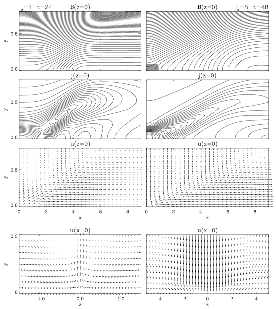
Figure 1: Magnetic field, current density, and velocity in the plane $z=0$, and velocity in the plane $x=0$ for run 1 ($l_{z}=1$) at $t=24$ (left panels) and for run 2 ($l_{z}=8$) at $t=48$ (right panels). The maximum outflow velocities are $\max(u_{x})=0.23$ for both runs. The gray shaded area is the region where anomalous resistivity is excited. The peak values of the velocity components in the bottom panels are $|u_{y}|\approx 0.02$ and $u_{z}\approx 0.1$ for both runs. (Peak velocities for run 2 at $t=24$ are about half the values given here.) Peak current densities are $\max(j)=1.7$ (run 1) and $\max(j)=3.0$ (run 2).

Figure 1 shows the evolution of the Harris sheet at characteristic times for $l_{z}=1$ and $l_{z}=8$, using $\beta=0.15$ and $v_{cr}=3$. In the system with $l_{z}=1$ (run 1 in Table I) the flow $u_{y}$ is already reversed (directed away from the reconnection region) by the inertia of the $u_{z}$ inflow and reconnection has already stopped by $t=24$. Also the field lines in the plane $z=0$ no longer possess the pure X-type topology, characteristic of reconnection, which was enforced during the initial perturbation ($t<t_{0}=10$). No anomalous resistivity occurs in this run after $t=t_{0}$, and characteristic quantities, such as the outflow velocity and the current density, decrease subsequently. In contrast, for $l_{z}=8$ (run 2 shown at $t=48$) the field lines and the flow in the plane $z=0$ are identical to the picture known from 2D systems after those have evolved into the fast reconnection regime, where anomalous resistivity is again excited. Also the current density ridges near the separatrices of the magnetic field are clearly developed, with the maxima of $j=|{\bf{j}}|$ and $\eta_{an}$ lying at ${\bf{x}}=0$. The maximum outflow velocity $\max(u_{x})$ rises continuously until it becomes Alfvénic at $t\!\approx\!160$ — before the boundary at $|x|=90$ is reached.

Runs 1 and 2 are in general agreement with the results of Ugai and Shimizu.[28] The removal of the pair of oppositely directed current sheets at the upper and lower boundary of the numerical box and the more gentle profile of the current density in the Harris equilibrium used here raise the minimum elongation of the initial resistivity, for the development of fast reconnection, somewhat to a value $l_{z}^{*}\sim 8$. The need to search for parameter settings that render such a strong requirement unnecessary is thus even strengthened.

Simply enlarging the $x$ extent of the perturbation ($l_{x}$) does not support the development of fast reconnection since the initial configuration is then closer to the Sweet-Parker configuration. This possesses smaller reconnection rates than a configuration with more localized resistivity (runs 4 and 5 in Table I; see also Sec. III.4). Applying the initial perturbation for a longer time appears to be reasonable because the collisional time scale, at which spontaneously created anomalous resistivity is expected to decay, can be much longer than the Alfvén transit time $\tau_{A}$ of the thin sheets forming in cosmic plasmas. However, this does not change the result for $l_{z}=1$: if the initial perturbation is applied for a longer time (e.g., $t_{0}=30$), the reversal of the flow $u_{y}$ and a transition from X-type to O-type magnetic topology occur before the perturbation is switched off, and again no anomalous resistivity is excited afterwards.

Another obvious modification consists in lowering the threshold $v_{cr}$ for the onset of anomalous resistivity. This parameter is usually set at an intermediate value for numerical convenience, to both enable recurrence of anomalous resistivity and to avoid its excitation over widespread regions of the box. A typical value in two-dimensional simulations is $v_{cr}=3$. From a physical point of view, a low value of $v_{cr}$ only slightly exceeding unity would be most reasonable for a study of spontaneous reconnection in cosmic plasmas, since it corresponds to a configuration in which the gradient scales in $x$ and $z$ are much larger than the current sheet width and the onset of resistivity enhancement in one place results from small fluctuations or a slight systematic inhomogeneity. We have therefore integrated the system with $l_{z}=l_{x}=l_{y}=0.8$ using $v_{cr}=1.1\mbox{--}1.5$ and obtained similar dynamical behavior in this whole range, including re-excitation of anomalous resistivity. This counteracts the general diffusion that dominated run 1 and enables build-up of a long-lasting spontaneous fast reconnection regime. The structures and dynamics in this case are only partly similar to the 2D system and will be explored further by run 3 in subsequent sections.

Finally, we consider very small values of $\beta$ permitting higher compressibility of the plasma. This should render excitation of anomalous resistivity according to Eq. (12) easier, since a higher pile-up of magnetic flux and current density, and stronger density reductions, are enabled. It turns out, however, that reducing $\beta$ below our standard value of 0.15 leads to only a minor increase (less than one per cent) of the maximum electron-ion drift velocity that is attained during the evolution. Generally, the influence of the plasma beta on the evolution of the considered systems has been found to be very weak in the range $\beta=0.0015-1.5$ (runs 6–8 in Table I).

Summarizing this parametric search, we find that appropriate setting of the threshold for the onset of anomalous resistivity enables the build-up of spontaneous reconnection in the case of an isotropic initial perturbation.

III.3 Structure of the reconnection region with a central X-line

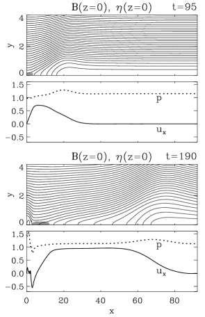
Figure 8: Magnetic field lines in the plane $z\!=\!0$ and the profiles $p(x,0,0)$ and $u_{x}(x,0,0)$ for run 2 at $t\!=\!95$ (top panels) and at $t\!=\!190$ (bottom panels). The region of anomalous resistivity is shown shaded.

First we discuss the case $l_{z}=8$ (run 2). The three-dimensional structure of the current sheet at times of a fully developed fast reconnection regime shows that the dynamics is surprisingly well confined to a slab $|z|\lesssim 2\,l_{z}$ around the $z=0$ plane. This is a consequence of the inflow $u_{z}$, which continues as long as the central X-line exists and inhibits spreading of the reconnection process in $z$, of the absence of a guide field component, and of the neglect of viscosity (which is reasonable for dilute cosmic plasmas). Magnetic field lines outside of this slab do not show the X-type topology, as can be seen in Fig. 2 at $t=95$. The bending of the field lines within the current sheet ($y<1$) reflects the inflow $u_{z}$ along the $z$ axis and the diversion of the outflow around the pressure maximum (“plasmoid” structure) which is pushed outward by the main reconnection outflow $u_{x}$. The outflow becomes Alfvénic at the rear side of the outgoing plasmoid (see below, Fig. 8).

The isosurfaces of the current density displayed in Fig. 3 for run 2 show the slab-like character of the system perhaps most clearly: the sheet remains practically undisturbed at $|z|\gtrsim 2\,l_{z}$ [Figs. 3(a) and 3(b)]. Within $|z|\lesssim l_{z}/2$ and between the pair of plasmoids ($|x|\lesssim 15$ at $t=95$) the structure is nearly two-dimensional. The cut at $z=0$ reveals the current density ridges (slow mode shocks) known from 2D reconnection. The occurrence of enhanced resistivity is much more localized at the origin than the regions of high current density and does not extend along the current density ridges (see Figs. 1, 7, and 8). This is due to the rarefaction of the plasma at the origin, which enters into the velocity-based criterion for resistivity enhancement. Thus, the essential features of Petschek’s reconnection model (Alfvénic outflows, localized resistivity enhancement at a central X-line, and slow mode shocks) are set up for $l_{z}>l_{z}^{*}$ within the nearly two-dimensional slab.

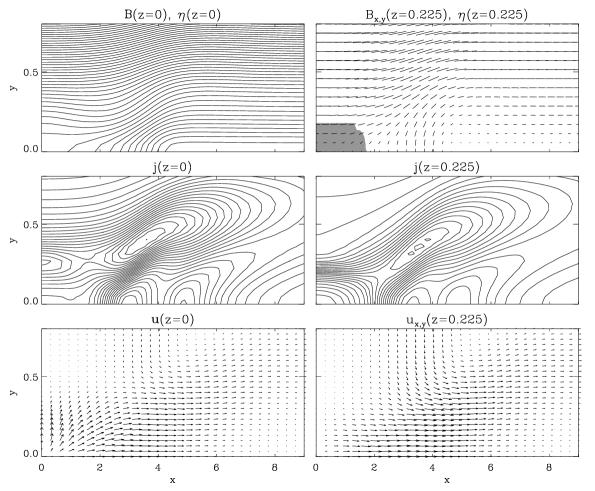
Figure 4: Magnetic field, current density, and velocity for run 3 ($l_{z}=0.8$) at $t=24$ in the plane $z=0$ (left panels) and in the plane $z=z_{1}=0.225$, which contains the maximum of $\eta_{an}$ at this time (right panels). Anomalous resistivity (gray shaded) is excited only for $z\neq 0$ at this time. Peak velocities are $u_{x}(z\!=\!0)=0.25$, $u_{y}(z\!=\!0)=0.034$, $u_{x}(z\!=\!z_{1})=0.22$, $u_{y}(z\!=\!z_{1})=-0.01$. Peak current densities are $\max[j(z\!=\!0)]=1.3$ and $\max[j(z\!=\!z_{1})]=1.8$.

The configuration formed from an isotropic initial perturbation is more complicated and only partly similar to the Petschek configuration. In run 3 ($l_{z}=0.8$, $v_{cr}=1.5$) anomalous resistivity is never excited at ${\bf x}=0$. Instead, oblique flows and flux pile-up by the inflow $u_{z}$ lead to a symmetric double structure with maxima of $\eta$ initially lying at the $z$ axis slightly inward of the point of maximum slope of the initial resistivity perturbation profile; the point $z_{1}$ of maximum $\eta$ lies in the range $|z|\approx 0.2$–0.4 for $14<t<72$. An inflow $u_{y}(y>0)<0$ is built up at the maxima of $\eta$, leading to a Petschek-like structure of reconnection in a neighborhood of the planes $|z|=z_{1}$. A magnetic X-configuration with the corresponding $x$-$y$ flow and the classical current density ridges exists there temporarily. These two slabs form a sandwich-like structure about the midplane $z=0$, in which the flow along the $y$ axis is reversed, $u_{y}(y>0)>0$, and reconnection is inhibited (Fig. 4). The outflow $u_{x}$ that results from the initial perturbation and the current density ridges extend between the slabs through the plane $z=0$. The available numerical resolution does not permit a clear distinction between whether the X-line continues through $z=0$ or an O-line is formed at $|z|\ll z_{1}$ already in this early phase.

The profiles along the $z$ axis of pressure, density, and velocity in Fig. 5 show the flow, driven by the pressure gradient $-\partial_{z}p/2$, at characteristic times for runs 2 and 3. The structures are similar in both runs with spatial scales being of the order $l_{z}$ during the Petschek-like phase.

III.4 Secondary tearing and long-term evolution

The plot of the electric field at the X-lines in Fig. 6 shows the temporal evolution of the reconnection process. We refer to $R={\eta}j$ as the reconnection rate in our system with $B_{z}(t\!=\!0)=0$, where the X-lines are magnetic nulls. Runs 2 and 3 and a two-dimensional comparison run are shown. The latter has physical and numerical parameters identical to run 2, except for the use of a uniform grid with resolutions $\Delta x_{0}$ and $\Delta y_{0}$ as given in Table I for run 2. Again we begin with a discussion of run 2. The reconnection rate at the X-line formed at ${\bf x}=0$ develops a single, well-defined peak (thick continuous lines in Fig. 6) which is of similar magnitude and shape for $l_{z}=8$ and $l_{z}=\infty$. Most importantly, $R$ does not stabilize after a Petschek-like configuration is established, but shows a monotonic decay with a decay time comparable to the rise time. This is in contradiction to the conclusions of Ugai and Shimizu[28] who had found some indications in favor of build-up of a quasi-steady reconnection regime (the rate of change of the flows and of the peak anomalous resistivity began to decrease over a period of $\sim 10\tau_{A}$ at the end of their run). Our calculation in a larger box over a longer period shows that, in fact, a quasi-steady state is not reached. Ugai and Shimizu have argued that a balance between convection of field lines by the inflow $u_{y}$ and magnetic diffusion is reached at the central X-line because $\eta=\eta(j/\rho)$ is permitted to rise freely, which enables a (quasi-) steady state of reconnection in 3D as well as in 2D. Their argument implicitly relies on the reconnection geometry in the $x$-$y$-plane being stationary. However, the structure of the current sheet in the neighborhood of the X-line evolves during the build-up of the reconnection regime. It is the evolution of the volume where anomalous resistivity is excited which leads to a decrease of the reconnection rate at ${\bf x}=0$ in the long-term evolution.

Figure 7 shows profiles along the $x$ axis of $j$, $\rho$, and the resulting anomalous resistivity $\eta_{an}$, for run 2. The regions of enhanced $j(x)$ and $\eta_{an}(x)$ at the origin broaden with time considerably. At the same time, the width of the corresponding profiles along the $y$ axis stays roughly constant, due to the inflow $u_{y}$. With anomalous resistivity extending to $|y|\approx 0.2$, the aspect ratio of the $\eta_{an}$ area has reached a value $\delta x_{\eta}/\delta y_{\eta}=33$ by $t=127$. Essentially, the inner section of the current sheet has undergone a transition from a Petschek configuration to a Sweet-Parker configuration. Consequently, the reconnection of field lines and the level of anomalous resistivity drop, primarily at the origin (where the pull by the outflow $u_{x}$ becomes weaker than at the ends of the extended $\eta_{an}$ area). Two symmetric maxima of the $\eta_{an}$ profile remain, which immediately lead to the formation of a pair of new magnetic X-lines at $t\approx 150$. An inflow along the $z$ direction is created also at the new X-lines, but it has only a weak effect because the reconnection inflow $u_{y}$ is already present at a larger scale. The outflow from the new X-lines drives a transition of topology at the origin, where an O-line is created. This change of topology is enabled by the still existing (although rapidly decaying) anomalous resistivity at ${\bf x}=0$. The reconnection rate in run 2 drops from $R=1.6\times 10^{-2}$ at $t=95$ to $R=8.4\times 10^{-3}$ at $t=152$. The Sweet-Parker reconnection rate, based on $\delta x_{\eta}$ and the average value $\langle\eta_{an}\rangle_{\delta x_{\eta}}$, is found to drop similarly, $R_{SP}(t\!=\!95)=2.9\times 10^{-2}$ and $R_{SP}(t\!=\!152)=1.6\times 10^{-2}$, thus supporting our interpretation. In comparison, the Petschek reconnection rate, based on the $x$ extent of the Petschek-like configuration (i.e., the $x$ extent of the current density ridges behind the outgoing plasmoid) and $\langle\eta_{an}\rangle_{\delta x_{\eta}}$, stays approximately constant, $R_{P}(t\!=\!95)=4.4\times 10^{-2}$ and $R_{P}(t\!=\!152)=4.1\times 10^{-2}$.

The creation of the pair of new X-lines has been found in 2D simulations of spontaneous reconnection and termed secondary tearing.[31] The evolution of the 3D system investigated here is similar to the 2D results. We remark that the inflow $u_{z}$, which peaks at the $z$ axis, supports the topology change at the origin by its tendency to revert the flow $u_{y}$. This is particularly true for small values of $l_{z}$ (see below). It has been argued[33] that secondary tearing only occurs if the model for $\eta_{an}$ is based on the current density and does not occur if the model is based on the electron-ion drift velocity. In the latter case, the density minimum at the origin was supposed to lead to a permanent localization of the anomalous resistivity. However, with the increasing extent of the anomalous resistivity area, the density minimum becomes progressively flatter, and the evolution is similar, only somewhat delayed, for the drift velocity criterion. Secondary tearing occurred in all runs which exhibited spontaneous re-excitation of anomalous resistivity (for various parameter settings in addition to Table I) at late stages ($t\gtrsim 150$).

The plot of the field lines and of the profiles $u_{x}(x)$ and $p(x)$ for run 2 in Fig. 8 demonstrates that the secondary tearing is not caused by the open boundary in the outflow direction ($|x|=L_{x}$): it occurs at a time when the disturbance created by the initial resistivity perturbation has not yet reached that boundary. It is also not caused by the nonuniformity of the grid, since the new X-line is formed at $x\approx 5$ while the grid is uniform for $|x|<10$ (Table I).

The topology change connected with the secondary tearing does not inhibit fast magnetic reconnection, instead it leads to re-amplification of the process. The reconnection rate remains variable because the plasmoid in the center of the system, which is permanently driven by the outflow from the new X-lines, executes oscillatory motions (it may even tear and merge again, as indicated in Fig. 8 at $t=190$ and by the small peak in the second panel of Fig. 6 at the same time) and because the $\eta_{an}$ area continues to show a slight tendency to elongate outwards in a time-variable manner. Both effects lead to variations of $\eta_{an}$ at the new X-lines. Repeated secondary tearing of this elongated current sheet section, typical of the 2D system (see the third panel of Fig. 6 and Ref. 31), occurs only once ($t=500\mbox{--}540$) and is of minor dynamical importance. Obviously this effect requires even larger $l_{z}$ because the tearing mode is most easily excited as a 2D instability[34] (although its nonlinear development may be three-dimensional[35]). Increasing numerical diffusion in the nonuniform part of the grid ($|x|>10$) may also have an influence.

A plasmoid with continuously rising pressure is formed in the central O-line region by the outflow from the adjacent X-lines. This plasmoid relaxes primarily by setting up a pair of outflow jets along the $z$ axis. These outflow jets, which are strongly confined (roughly to the cross section of the plasmoid), are shown for run 2 in Fig. 9(a). Their velocity reaches $0.7\,V_{A}$ during $t=200\mbox{--}380$ (Fig. 5). In 2D the relaxation is only possible by slowly shifting the new X-lines outward along the $x$ axis.[31] Also the area of anomalous resistivity starts to grow in the $z$ direction, forming a pair of ropes at the surface of the plasmoid (Fig. 10). At the same time, the reconnection rate at the new X-lines decreases at the $x$ axis, since an increasing amount of field line bending is required to convect flux toward the new X-lines, which are staying close to the swelling plasmoid, and since the increasing pressure in the plasmoid resists the reconnection outflow from the new X-lines. This results in a splitting and displacement of the maxima of $\eta_{an}$ and $R$ off the $x$ axis along these ropes toward large values of $|z|$ after $t=450$. The second panel of Fig. 6 displays the decrease of the reconnection rate at $z=0$ as a continuous line and the global maximum of the reconnection rate as a dashed line. The latter is observed to stay almost constant in the short interval during which the maximum is displaced at high apparent velocity to the boundary $L_{z}$. The secondary tearing thus enables spreading of the reconnection process in the $z$ direction. However, the current limitation of grid sizes prevents a systematic investigation of this phase.

The time evolution of the reconnected flux in the first quadrant of the current sheet plane, $\Phi=\int B_{y}(x,0,z,t){\rm d}x{\rm d}z/\delta z_{\eta}(t)$, which is plotted in the bottom panel of Fig. 6, also indicates enhanced reconnection after secondary tearing and the spreading of the reconnection process in the $z$ direction. The “outer” reconnected flux ($\Phi_{o}<0$) between the dominant X-line and the boundary $x=L_{x}$ and the “inner” reconnected flux ($\Phi_{i}>0$), which accumulates between the dominant X-line and the $z$ axis after secondary tearing, are plotted separately. One has to keep in mind, however, that these quantities still carry signatures of several processes, which are difficult to disentangle and quantify. Both parts of the flux are influenced by convection across the boundaries $x=L_{x}$ or $z=L_{z}$. The area of integration, and consequently the proportion between $\Phi_{o}$ and $\Phi_{i}$, depend on the location of the dominant X-line, which is strongly shifted in the 2D run. Coalescence of magnetic islands after secondary tearing annihilates previously reconnected flux. Finally, there is some arbitrariness in the normalization of $\Phi$ for the 3D runs, required for the comparison with the 2D run: it can be done using $l_{z}$, $L_{z}$, or the instantaneous extent of the anomalous resistivity region $\delta z_{\eta}(t)$. Nevertheless, one can see that (1) maxima of ${\rm d}|\Phi|/{\rm d}t$ correspond to enhanced reconnection rates in the upper panels of the figure, (2) run 2 and the 2D run lead to comparable amounts of reconnected flux, (3) the flux $-\Phi_{o}$ peaks roughly at the time at which the rear side of the plasmoid that is created by the initial perturbation has reached the boundary $L_{x}$.

Turning now to the case of isotropic initial perturbation (run 3 with $l_{z}=0.8$), we find that the evolution is largely, but not fully, analogous to the case of anisotropic initial perturbation (run 2). Again, the Petschek-like configuration initially formed in the two symmetric slabs around $|z|=z_{1}$ turns out to be not a stable configuration. Figure 11 shows the evolution of the anomalous resistivity in the current sheet plane $y=0$, where the maximum of $\eta$ remains during the whole run. The initial elongation of the $\eta_{an}$ area in the direction of the outflow and the subsequent decrease of $\eta_{an}(x=0)$ are similar to run 2. The combined effect of the coherent outflow $u_{x}$, which extends over a larger $z$ interval than the anomalous resistivity and includes the plane $z=0$ (cf. Fig. 4), and the continuing inflow $u_{z}$ let the $\eta_{an}$ area then approach the $x$ axis. Secondary tearing in the plane $z=0$ occurs immediately ($t=72$), also being supported by the still reversed flow $u_{y}(0,y>0,0)>0$. A magnetic configuration identical to the one shown in the bottom panels of Fig. 8 is formed. The subsequent evolution is qualitatively similar to the case $l_{z}=8$, although the reconnection rate remains much smaller and is far less variable. This reflects the fact that here the driving reconnection at the new X-line is far less coherent in $z$ and the flows $u_{x,y,z}$ have to be partly reorganized in space. The reconnection rate was found to depend only weakly on the parameter $v_{cr}$ in the range $1.1\leq v_{cr}\leq 1.5$. The outflow jets along the $z$ axis are also formed [Figs. 5 and 9(b)]. The maximum outflow velocities are $u_{x}=0.8$ at $t\sim 400$ and $u_{z}=0.3$ at $t=300\mbox{--}450$. The splitting of the maximum resistivity in the $z$ direction and the subsequent rapid displacement of the maximum along the new X-lines to the boundary $|z|=L_{z}$ occurs at $t>310$. As in the case $l_{z}=8$, there is a strong tendency toward a quasi-2D configuration in the numerical box, based on the formation of $\eta_{an}$ ropes along the new X-lines (Fig. 11). In a larger system, it can be expected that the reconnection rate and the outflow velocities rise further as soon as the quasi-2D configuration extends over a sufficiently large interval $\Delta z\gg 1$ and the overall configuration becomes similar to run 2.

The secondary tearing is essential to reach a significant reconnection rate in the case of an isotropic initial perturbation, because it leads to growth of the area of anomalous resistivity in the $z$ direction.

III.5 Parallel current density and electric field

Field lines of ${\bf{j}}({\bf{x}})$ are displayed for run 2 in Fig. 12. These visualize the current diversion which is caused by the finite $z$-extent of both the resistivity region and the reconnection flows, $u_{x}$ and $u_{y}$. Lines of current flow starting close to the current sheet plane $y=0$ are diverted mainly in the $x$ direction, while lines starting at a certain distance from $y=0$ are diverted mainly in the $y$ direction, to form the current density ridges shown in Fig. 3. The current diversion is related to the generation of current components parallel to the magnetic field, which are of particular significance because the resulting parallel electric field, $E_{||}=\eta_{an}j_{||}$, may dominate the acceleration of particles and because the currents may be directly observable as the “substorm current wedge” in events of magnetospheric activity. Note that $E_{||}=j_{||}=0$ in the 2D evolution of neutral current sheets. The generation of parallel current components is caused by the plasma flow as well as by the existence of nonuniform (anomalous) resistivity. This can be seen by considering the current helicity density [36, 37]

$$h_{c}={\bf j}\cdot{\bf B}\,.$$

Its time derivative is related to a temporal change of the parallel current density. In dimensionless units:

$$\frac{\partial h_{c}}{\partial t} = \partial_{t}{\bf j}\cdot{\bf B}+{\bf j}\cdot\partial_{t}{\bf B}$$ (13)

$$= [{\boldmath\nabla\times}{\boldmath\nabla\times}({\bf u}{\boldmath\times}{\bf B})]\cdot{\bf B}$$

$$-\,[{\boldmath\nabla\times}{\boldmath\nabla\times}(\eta{\bf j})]\cdot{\bf B}$$

$$+\,[{\boldmath\nabla\times}({\bf u}{\boldmath\times}{\bf B})+\eta\,\Delta{\bf B}]\cdot{\bf j}\,.$$

The second term shows that contributions to the growth of $j_{||}$ result not only from the presence of resistivity but also from nonvanishing first and second spatial derivatives. The derivatives of $\eta$ are particularly important at large Lundquist numbers, where the terms proportional to $\eta$ become small. That these contributions are indeed essential can be seen in Fig. 13, where contours of $j_{||}$ and $\eta$ are plotted for run 2 ($l_{z}=8$) during the Petschek-like reconnection phase ($t=95$) and after secondary tearing has occurred ($t=190$). At both times the highest parallel current density components are created close to the surface of the region of nonvanishing resistivity, where the first and second derivatives of $\eta$ are both large. Figure 14(a) displays isosurfaces of $|j_{||}|$ for the same dataset ($t=190$) at two levels. The concentration of the highest parallel current densities close to the surface of the resistivity region is again apparent. The lower-level isosurface shows that the overall structure of the $j_{||}$ region follows the current density ridges seen in Fig. 3 and that there is a second region of enhanced parallel current components at the rear side of the outgoing plasmoid. Significant $j_{||}$ components are thus also created at lines of current flow far away from the resistivity region (cf. Fig. 12). The latter effect is due to the shear of the outflow, which is diverted around the outgoing plasmoid, and has been discussed in detail previously.[23, 24, 25] The highest parallel current densities occur as a result of secondary tearing ($t=180$–420 in run 2 and $t=350$–450 in run 3) at the surface of the central plasmoid close to the area of anomalous resistivity [Fig. 13 and Fig. 14(b)]. The maximum parallel current densities reached in run 2 [$\max(j_{||})=2.4\,j(0)$] and run 3 [$\max(j_{||})=2.1\,j(0)$] are comparable.

The parallel electric field peaks where the volumes of anomalous resistivity and high parallel current density intersect, i.e., at the surface of the central plasmoid close to the new X-lines after secondary tearing (Fig. 13). For both runs 2 and 3, the temporal maximum of $E_{||}$ is related to a strong oscillation of the central plasmoid, which tends to tear in the $x$ direction but merges again, $\max[E_{||}(x=4.0,y=0.09,z=3.5,t=197)]=1.3\times 10^{-3}$ in run 2 and $\max[E_{||}(2.7,0.7,0.6,352)]=1.7\times 10^{-3}$ in run 3.

IV CONCLUSIONS AND DISCUSSION

In this paper we have investigated, within the framework of one-fluid MHD, the three-dimensional dynamics of magnetic reconnection in a compressible Harris current sheet with initially antiparallel magnetic field and dynamically coupled resistivity. The three-dimensional development was initiated by applying a resistivity perturbation bounded in $x$, $y$, and $z$. Particular attention was paid to the question of the development of the so-called spontaneous fast reconnection regime. The results can be summarized as follows.

(1) The dynamical development depends strongly on the elongation $l_{z}$ of the initial perturbation in the $z$ direction relative to its dimensions $l_{x}$ and $l_{y}$. Only for sufficiently anisotropic resistivity profiles with $l_{z}>l_{z}^{*}>l_{x,y}$ will the inflow along the $z$ axis be sufficiently weak so that the reconnection inflow in the $y$ direction and a fast reconnection regime can develop in a manner similar to the two-dimensional case. For the Harris sheet with $l_{x}\!\sim\!l_{y}\!\sim\!1$ and $v_{cr}=3$, the critical elongation $l_{z}^{*}$ lies in the range 4–8. Over a period of $\sim 10^{2}\,\tau_{A}$, a Petschek-like reconnection regime is built up but remains bounded to a slab around the plane $z=0$, the width of which is approximately equal to twice the $z$ extent of the initial perturbation.

(2) The system is not able to sustain the Petschek reconnection regime in a (quasi-) steady manner, instead the region of anomalous resistivity at the X-line becomes increasingly elongated with time in the $x$ direction, thus temporarily resembling a Sweet-Parker configuration. This leads to a decrease of the reconnection rate in the region of the initial perturbation. As a result, the system shows a transition of topology known as secondary tearing, i.e., a symmetrical pair of X-lines is formed and the original X-line is replaced by an O-line. This process is supported in the three-dimensional case by the inflow along the $z$ axis and occurs even with the drift velocity-based criterion for resistivity enhancement. The secondary tearing leads to enhanced and time-variable reconnection, to a second pair of outflow jets directed along the O-line, and to expansion of the reconnection process along the newly formed X-lines in the $z$ direction.

(3) The requirement on the anisotropy of the initial perturbation can be relaxed by lowering the threshold for the excitation of anomalous resistivity substantially below the value commonly used in two-dimensional simulations. The system with an isotropic initial perturbation then evolves through a partly Petschek-like reconnection regime but experiences secondary tearing relatively early. Subsequently, the evolution proceeds in a qualitatively similar manner as in the case of a strongly anisotropic initial perturbation. With the expansion of the reconnection process along the new X-lines, significant reconnection rates are achieved after several $10^{2}$ Alfvén times.

(4) The three-dimensional reconnection process forms substantial current density components along the magnetic field, $\max[j_{||}({\bf x},t)]\approx 2.4\,j(0)$ for $l_{z}=8$ and $\approx 2.1\,j(0)$ for $l_{z}=0.8$. Their maximum lies at the surface of the plasmoid formed by secondary tearing near the boundary of the anomalous resistivity region (i.e., near the new X-lines). Also the maximum parallel electric field occurs near the new X-lines, within the region of anomalous resistivity. It is of order $E_{||}\sim(1\mbox{--}2)\times 10^{-3}$ and is rather insensitive to the elongation $l_{z}$ of the initial perturbation.

The choice of a strongly anisotropic perturbation ($l_{z}\gg l_{x}$ in run 2) has permitted a detailed comparison of the different phases of three-dimensional spontaneous resistive reconnection in initially antiparallel magnetic fields (neutral current sheets) with the two-dimensional case. However, as discussed already in the introduction, this configuration with the anisotropy oriented across the magnetic field is not expected to occur spontaneously (caused, e.g., by fluctuations in a marginally stable equilibrium) in cosmic plasmas. Possibly an ideal MHD instability can be found which enforces such a configuration. Simulations of the reconfiguration of an arcade of magnetic loops in the solar atmosphere[38] are suggestive in this direction and have been taken in the literature to justify two-dimensional models of the subsequent reconnection, but this particular instability requires a large guide field component.

Our study of spontaneous reconnection initiated by an isotropic perturbation ($l_{x}=l_{y}=l_{z}$ in run 3) required that a lower threshold for the onset of anomalous resistivity be chosen than commonly used in 2D simulations, which, however, appears physically reasonable. Although this system did not show all the attributes of “fast Petschek-like reconnection,” substantial reconnection rates were achieved at least over several $10^{2}\,\tau_{A}$ and clear indications have been obtained that the reconnection process also spreads in the $z$ direction to become a large-scale disturbance. This suggests that three-dimensional fast reconnection may occur spontaneously and lead to macroscopic energy release events in neutral current sheets.

As a further possibility to trigger long-lasting, large-scale, and possibly fast magnetic reconnection by a three-dimensionally localized initial perturbation, one has to consider a sheared current sheet with a nonvanishing guide field ($B_{z}(t\!=\!0)\neq 0$). In that case an anisotropy $l_{z}\gg l_{x}$ of the resistivity perturbation would be oriented along the magnetic field in the center of the current sheet ($y=0$) and can therefore be expected to occur spontaneously. Three-dimensional magnetic reconnection in such a sheared field configuration, where the midplane reflection symmetry is broken and the dynamics is strongly modified in comparison to the system considered here, will be investigated in a future paper.

Finally, a long-lasting and possibly steady regime of three-dimensional fast reconnection may be obtained by prescribing an inflow toward the sheet,[39] similar to two-dimensional simulations.[40] The inflow $u_{y}(|y|\to\infty)$ may be relatively weak, since rather low values of $u_{y}$ [$\sim(1\mbox{--}3)\times 10^{-2}$] occurred in our simulations even at times of peak reconnection rates. Such driven reconnection is expected to occur at the dayside of the magnetosphere and possibly at the boundary of newly emerging magnetic flux in coronae.

The long-term evolution of three-dimensional spontaneous reconnection has been investigated here under the constraint of symmetry with respect to the planes $x=0$, $y=0$, and $z=0$, dictated by practical limitations of three-dimensional grid sizes. Strong symmetric outflows $u_{x}$ and $u_{z}$ have been found. It is conceivable that asymmetries with respect to $x=0$ or $z=0$ would lead to predominantly one-sided outflows $u_{x}$ or $u_{z}$, respectively, and to a different long-term evolution. For weak asymmetries the ejection of the plasmoid formed through secondary tearing may occur. This effect has been seen in two-dimensional simulations[41, 32] and will be studied in 3D as well.

The growth of the region of anomalous resistivity into the direction of the reconnection outflow $u_{x}$ turned out to be an essential element of the dynamics that leads to secondary tearing and subsequent growth of the perturbation into the $z$ direction. This effect is related to the inability of the fluid (at least in standard MHD) to carry a sufficient amount of magnetic flux into a strongly localized diffusion region to support the Alfvénic outflow of reconnected flux in steady state.[29] Higher inflow velocities into the diffusion region occur in more general fluid or kinetic treatments of collisionless and resistive reconnection,[17, 19] where separate electron and ion scales form. How these faster flows match to the outer regions, where the electrons and ions are coupled, and thus the question of whether the growth of the diffusion region is enforced by the large-scale flow pattern irrespective of its microscopic physics, requires further investigation.

Table I: Parameters of the three-dimensional simulation runs. The resolutions $\Delta x_{0}$, $\Delta y_{0}$, $\Delta z_{0}$ refer to the inner uniform part of the nonequidistant grid, whose size is given by $L_{x}^{\prime}$, $L_{y}^{\prime}$, and $L_{z}^{\prime}$.

Run	$l_{x}$	$l_{z}$	$v_{cr}$	$\beta$	$L_{x}$	$L_{y}$	$L_{z}$	$\Delta x_{0}$	$\Delta y_{0}$	$\Delta z_{0}$	$L_{x}^{\prime}$	$L_{y}^{\prime}$	$L_{z}^{\prime}$	$\eta_{an}(t\!>\!t_{0})$
1	0.8	1	3	0.15	20	4	25	0.10	0.045	0.075	3	1	2	no
2	0.8	8	3	0.15	90	4	40	0.10	0.045	0.25	10	1	3	yes
3	0.8	0.8	1.5	0.15	90	4	10	0.10	0.045	0.025	10	1	1.3	yes
4	4.0	1	3	0.15	40	4	20	0.10	0.045	0.1	3	2	3	no
5	16.0	1	3	0.15	40	4	20	0.10	0.045	0.1	3	2	3	no
6	0.8	1	3	0.015	20	4	25	0.10	0.045	0.075	3	1	2	no
7	0.8	1	3	0.0015	20	4	25	0.10	0.045	0.075	3	1	2	no
8	0.8	1	3	1.5	20	4	25	0.10	0.045	0.075	3	1	2	no

Figure 2: Magnetic field lines passing through $x=30$ and $z=0,\,l_{z},\,2l_{z}$, respectively, for run 2 ($l_{z}=8$) at $t=95$.

Figure 3: Surfaces of constant current density $j=|{\bf{j}}|$ for run 2 ($l_{z}=8$). (a) The 20 per cent level of $\max(j)=4.0$ (located at the origin) at $t\!=\!95$. (b) The 10 per cent level of $\max(j)=5.8$ (located at the origin) at $t\!=\!190$ (before plasmoid ejection). (c) The 10 per cent level of $\max(j)=4.9$ located at the new X-lines at $t\!=\!354$ (after plasmoid ejection).

Figure 5: Profiles of the pressure (solid lines), density (dotted), and velocity (dashed) for runs 2 (top panel) and 3 (bottom panel) at a time of Petschek-like reconnection (thick lines) and after secondary tearing (thin lines).

Figure 6: Reconnection rates versus time for run 3 (top), run 2 (second panel), and the 2D comparison run (third panel). Rates at different X-lines are shown separately. Solid lines show reconnection rates at the $x$ axis, dashed lines show maximum reconnection rates occurring off the $x$ axis but within the box, dotted lines refer to maximum reconnection rates occurring at the boundary $|z|=L_{z}$. Thick lines refer to reconnection with a central X-line (Petschek-like), an intermediate line width is used for reconnection rates after secondary tearing. The initial perturbation is included as a thin line. The narrow and weak secondary peak in run 2 at $t\approx 190$ results from magnetic island coalescence at ${\bf x}=0$. Bottom panel: reconnected flux $\Phi$ for $l_{z}=\infty$ (solid lines), $l_{z}=8$ (dotted), and $l_{z}=0.8$ (dashed). Thin lines ($\Phi<0$) refer to the reconnected flux outward of the dominant X-line, thick lines ($\Phi>0$) refer to the reconnected flux between the dominant X-line and the $z$ axis after secondary tearing.

Figure 7: Profiles of resistivity $\eta$ (thick line), current density $j$ (thin line), and mass density $\rho$ (dotted) along the $x$ axis for run 2 at different times.

Figure 9: (a) Isosurface $|{\bf u}|\!=\!0.5$ in run 2 at $t=240$ showing pairs of outflow jets along the $x$ and $z$ axes. (b) Isosurface $|{\bf u}|\!=\!0.3$ for run 3 at $t=320$ showing similar jets.

Figure 10: Volume of anomalous resistivity delineating the magnetic X-lines in run 2 at $t=480$, where maximum reconnection occurs at $|z|=2.75$.

Figure 11: Evolution of anomalous resistivity in the current sheet plane for run 3 ($l_{z}=0.8$).

Figure 12: Lines of current flow (thick lines) and their projections onto the $x$-$y$-plane (thin lines) for run 2 ($l_{z}=8$) at $t=95$. The lines start either at $y=0.07$ or at $y=-0.6$ at the bottom of the box.

Figure 13: Contours of $|j_{\parallel}|$ (thin lines) and $\eta_{an}$ (thick lines) for run 2 in the planes containing the maximum $|j_{\parallel}|$ during the Petschek-like phase ($t=95$) and after secondary tearing ($t=190$). Run 3 yields a similar picture (not shown).

Figure 14: (a) Isosurface of $|j_{\parallel}|$ for run 2 at $t=190$. The 14 per cent level is displayed in the left half of the box ($x<0$), and the 7 per cent level is displayed in the right half ($x>0$). The maximum parallel current density is $j_{\parallel}(x=2.4,y=0.13,z=1.75,t=190)=1.4\,j(0)$. (b) The same for run 3 at $t=384$ [4 per cent of $\max(j_{\parallel})=j_{\parallel}(1.7,0.8,0.2,384)=2.1\,j(0)$].