Eclipse Mapping of the Accretion Stream in UZ Fornacis

Abstract

We present a new method to map the surface brightness of the accretion streams in AM Herculis systems from observed light curves. Extensive tests of the algorithm show that it reliably reproduces the intensity distribution of the stream for data with a signal-to-noise ratio $\ga 5$. As a first application, we map the accretion stream emission of C iv $\lambda$ 1550 in the polar UZ Fornacis using HST FOS high state spectra. We find three main emission regions along the accretion stream: (1) On the ballistic part of the accretion stream, (2) on the magnetically funneled stream near the primary accretion spot, and (3) on the magnetically funneled stream at a position above the stagnation region.

1 Introduction

Polars, as AM Hers are commonly named due to their highly polarized emission, consist of a late type main-sequence star (red dwarf, secondary star) and a highly magnetized white dwarf (WD, primary star). The red dwarf, filling its Roche volume, injects matter through the $L_{1}$ point into the Roche volume of the WD. Unlike in non-magnetic systems, this material does not form an accretion disc, but couples onto the magnetic field once the magnetic pressure exceeds the ram pressure. From this stagnation region ($SR$) on, the accretion stream follows a magnetic field line until it impacts onto the white dwarf surface. For a review of polars, see Warner Warner (1995).

In systems with an inclination $i\ga 70\degr$, the secondary star gradually eclipses the accretion stream during the inferior conjunction. Using tomographical methods, it is – in principle – possible to reconstruct the surface brightness distribution on the accretion stream from time resolved observations. This method has been successfully applied to accretion discs in non-magnetic CVs (“eclipse mapping”, Horne Horne (1985)). We present tests and a first application of a new eclipse mapping code, which allows the reconstruction of the intensity distribution on the accretion stream in magnetic CVs.

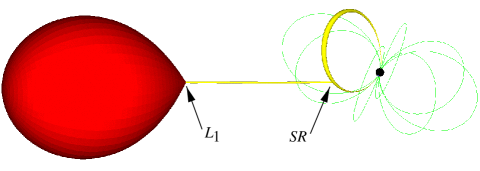
Figure 1: Overview of our 3d-Model of a polar. $L_{1}$ marks the inner lagrangian point, $SR$ the position of the stagnation or coupling region.

Similar attempts to map accretion streams in polars have been investigated by Hakala Hakala (1995) and Vrielmann and Schwope Vrielmann and Schwope (1999) for HU~Aquarii. An improved version of Hakala’s Hakala (1995) method has been presented by Harrop-Allin et al. Harrop-Allin et al. (1999b) with application to real data for the system HU Aquarii Harrop-Allin et al. (1999a). A drawback of all these approaches is that they only consider the eclipse of the accretion stream by the secondary star. In reality, the geometry may be more complicated: the far side of the magnetically coupled stream may eclipse stream elements close to the WD, as well as the hot accretion spot on the WD itself. The latter effect is commonly observed as a dip in the soft X-ray light curves prior to the eclipse (e.g. Sirk and Howell, 1998). The stream-stream eclipse may be detected in data which are dominated by emission from the accretion stream, e.g. in the light curves of high-excitation emission lines where the secondary contributes only little to the line flux.

Here, we describe a new accretion stream eclipse mapping method, using a 3d code which can handle the full complexity of the geometry together with an evolution strategy as fit algorithm. We present extensive tests of the method and map as a first application to real data the accretion stream in UZ For emission of C iv $\lambda$ 1550.

2 The 3d Cataclysmic Variable Model

Our computer code CVMOD generates $N$ small surface elements (convex quadrangles, some of which are degenerated to triangles), which represent the surfaces of the individual components of the CV (WD, secondary, accretion stream) in three-dimensional space (Fig. 1). Using simple rotation algorithms, the position of each surface element $i=1\dots N$ can be computed for a given orbital phase $\Phi$.

The white dwarf is modelled as an approximated sphere, using surface elements of nearly constant area Gänsicke et al. (1998). The secondary star is assumed to fill its Roche volume. Here, the surface elements are choosen in such a way that their boundaries align with longitude and latitude circles of the Roche surface, taking the $L_{1}$-point as the origin.

We generate the surface of the accretion stream in two parts, (a) the ballistic part from $L_{1}$ to $SR$, and (b) the dipole-part from $SR$ to the surface of the white dwarf.

(a) For the ballistic part of the stream, we use single-particle trajectories. The equations of motion in the corotating frame are given by

$$\ddot{x} = +\mu\frac{x-x_{1}}{r_{1}^{3}}-(1-\mu)\frac{x-x_{2}}{r_{2}^{3}}+2\dot{y}+x$$ (1)

$$\ddot{y} = -\mu\frac{y}{r_{1}^{3}}-(1-\mu)\frac{y}{r_{2}^{3}}-2\dot{x}+y$$ (2)

$$\ddot{z} = -\mu\frac{z}{r_{1}^{3}}-(1-\mu)\frac{z}{r_{2}^{3}}$$ (3)

Equation (3) has been added to Flannery’s Flannery (1975) set of two-dimensional equations. $\mu=(M_{1}+M_{2})/M_{1}$ is the mass fraction of the white dwarf, $r_{1}$ and $r_{2}$ are the distances from the point $(x,y,z)$ to the white dwarf and the secondary, respectively, in units of the orbital separation $a$. The coordinate origin is at the centre of gravity, the $x$-axis is along the lines connecting the centres of the stars, the system rotates with the angular frequency $\omega$ around to the $z$-axis. The velocity $\boldsymbol{v}=(\dot{x},\dot{y},\dot{z})$ is given in units of $a\omega$, $\boldsymbol{v_{0}}=(\dot{x}_{0},\dot{y}_{0},\dot{z}_{0})$ is the initial velocity in the $L_{1}$ point.

If $\dot{z}_{0}=0$, the trajectories resulting from the numerical integration of eq. (1) – (3) are restricted to the orbital plane. However, calculating single-particle trajectories with different initial velocity directions (allowing also $\dot{z}_{0}\neq 0$) shows that there is a region approximately one third of the way downstream from $L_{1}$ to $SR$ where all trajectories pass within very small separations, corresponding to a striction of the accretion stream.

We define a 3d version of the stream as a tube with a circular cross section with radius $r_{\mathrm{Tube}}=5\times 10^{8}\,\mathrm{cm}$ centred on the single-particle trajectory for $\dot{x}=10\,\mathrm{km}\,\mathrm{s}^{-1},\dot{y}=\dot{z}=0$.

(b) When the matter reaches $SR$, we switch from a ballistic single-particle trajectory to a magnetically forced dipole geometry. The central trajectory is generated using the dipole formula $r=\boldsymbol{r_{0}}\sin^{2}\alpha$, where $\alpha$ is the angle between the dipole axis and the position of the particle $(r,\varphi,\alpha)$. This can be interpreted as the magnetic field line $F$ passing through the stagnation point $SR$ and the hot spots on the WD. Knowing $F$, we assume a circular cross section with the radius $r_{SR}=r_{\mathrm{Tube}}=5\times 10^{8}\,\mathrm{cm}$ for the region where the dipole intersects the ballistic stream. This cross section is subject to transformation as $\alpha$ changes. Thus, the cross section of the stream is no longer constant in space but bounded everywhere by the same magnetic field lines.

Our accretion stream model involves several assumptions: (1) The cross section of the stream itself is to some extent arbitrary because we consider it to be – for our current data, see below – essentially a line source. (2) The neglect of the magnetic drag King (1993); Wynn and King (1995) on the ballistic part of the stream and the neglect of deformation of the dipole field cause the model stream to deviate in space from the true stream trajectory. While, in fact, the location of $SR$ may fluctuate with accretion rate (as does the location of the Earth’s magnetopause), the evidence for a sharp soft X-ray absorption dip caused by the stream suggest that $SR$ does not wander about on time scales short compared to the orbital period. (3) The abrupt switch-over from the ballistic to the dipole part of the stream may not describe the physics of $SR$ correctly. This discrepancy, however, does not seriously affect our results, because the eclipse tomography is sensitive primarily to displacements in the times of ingress and egress of $SR$ which are constrained by the absorption dip in the UV continuum (and, in principle, in soft X-rays). The $\approx 5\,\mbox{sec}$ time bins of our observed light curves correspond to $\approx 10^{8}\,\mbox{cm}$ in space at $SR$. Hence, our code is insensitive to structure on a smaller scale. In fact, the smallest resolved structures are much larger because of the noise level of our data. While our approach clearly involves several approximations, it is tailored to the desired aim of mapping the accretion stream from the information obtained from an emission line light curve.

In our current code, we restrict the possible brightness distribution so that for each stream segment, which consists of 16 surface elements forming a section of the tube-like stream, the intensity is the same, i.e. there is no intensity variation around the stream. For the current data, this is no serious drawback, since we only use observations covering a small phase interval around the eclipse. Our results refer, therefore, to the stream brightness as seen from the secondary. From the present observations we can not infer how the fraction of the stream illuminated by the X-ray/UV spot on the WD looks like. The required extension of our computer code, allowing for brightness variation around the stream, is straightforward. The present version of the code is, however, adapted to the data set considered here.

3 Light curve fitting

The basic idea of our eclipse mapping algorithm is to reconstruct the intensity distribution on the accretion stream by comparing and fitting a synthetic light curve to an observed one. The comparison between these light curves is done with a $\chi^{2}$-minimization, which is modified by means of a maximum entropy method. Sections 3.1 describes the light curve generation, 3.2 the maximum entropy method, and 3.3 the actual fitting algorithm.

3.1 Light curve generation

In order to generate a light curve from the 3d model, it is neccessary to know which surface elements $i$ are visible at a given phase $\Phi$. We designate the set of visible surfaces $V(\Phi)$.

In general, each of the three components (WD, secondary, accretion stream) may eclipse (parts of) the other two, and the accretion stream may partially eclipse itself. This is a typical hidden surface problem. However, in contrast to the widespread computer graphics algorithms which work in the image space of the selected output device (e.g. a screen or a printer), and which provide the information ‘pixel $j$ shows surface $i$’, we need to work in the object space, answering the question ‘is surface $i$ visible at phase $\Phi$?’. For a recent review on object space algorithms see Dorward Dorward (1994). Unfortunately, there is no readily available algorithm which fits our needs, thus we use a self-designed 3d object-space hidden-surface algorithm. Let $N$ be the number of surface elements of our 3d model. According to Dorward Dorward (1994), the time $T$ needed to perform an object space visibility analysis goes like $T\propto N\log N\dots N^{2}$. Our algorithm performs its task in $T\propto N^{1.5\dots 1.8}$, with the faster results during the eclipse of the system. It is obviously necessary to optimize the number of surface elements in order to minimize the computation time without getting too coarse a 3d grid.

Once $V(\Phi)$ has been determined, the angles between the surface normals of $i\in V(\Phi)$ and the line of sight, and the projected areas $A_{i,\Phi}$ of $i\in V(\Phi)$ are computed. Designating the intensity of the surface element $i$ at the wavelength $\lambda$ with $I_{i,\lambda}$, the observed flux $F_{\lambda}(\Phi)$ is

$$F_{\lambda}(\Phi)=\sum\limits_{i\in V(\Phi)}I_{i,\lambda}A_{i}(\Phi)$$ (4)

Here, two important assumptions are made: (a) the emission from all surface elements is optically thick, and (b) the emission is isotropic, i.e. there is no limb darkening in addition to the foreshortening of the projected area of the surface elements. The computation of a synthetic light curve is straightforward. It suffices to compute $F_{\lambda}(\Phi)$ for the desired set of orbital phases.

While the above mentioned algorithm can produce light curves for all three components, the WD, the secondary, and the accretion stream, we constrain in the following the computations of light curves to emission from the accretion stream only. Therefore, we treat the white dwarf and the secondary star as dark opaque objects, screening the accretion stream.

3.2 Constraining the problem: MEM

In the eclipse mapping analysis, the number of free parameters, i.e. the intensity of the $N$ surface elements, is typically much larger than the number of observed data points. Therefore, one has to reduce the degrees of freedom in the fit algorithm in a sensible way. An approach which has proved successful for accretion discs is the maximum entropy method MEM Horne (1985). The basic idea is to define an image entropy $S$ which has to be maximized, while the deviation between synthetic and observed light curve, usually measured by $\chi^{2}/n$, is minimized ($n$ is the number of phase steps or data points). Let $D_{i}$ be

$$D_{i}=\frac{\sum\limits_{j=1}^{N}I_{j}\exp\left(-\frac{\displaystyle(\boldsymbol{r}_{i}-\boldsymbol{r}_{j})^{2}}{\displaystyle 2\Delta^{2}}\right)}{\sum\limits_{j=1}^{N}\exp\left(-\frac{\displaystyle(\boldsymbol{r}_{i}-\boldsymbol{r}_{j})^{2}}{\displaystyle 2\Delta^{2}}\right)}$$ (5)

the default image for the surface element $i$. Then the entropy is given by

$$S=\frac{\sum\limits_{i=1}^{N}I_{i}\left(\ln{\displaystyle\frac{I_{i}}{D_{i}}}-1\right)}{\sum\limits_{i=1}^{N}I_{i}}$$ (6)

In Eq. (5), $\boldsymbol{r}_{i}$ and $\boldsymbol{r}_{j}$ are the positions of the surface elements $i$ and $j$. $\Delta$ determines the range of the MEM in that the default image (5) is a convolution of the actual image with a Gaussian with the $\sigma$-width of $\Delta$. Hence, the entropy measures the deviation of the actual image from the default image. An ideal entropic image (with no contrast at all) has $S=1$. We use $\Delta=1\times 10^{9}\,\mbox{cm}\approx 0.02a$ for our test calculations and for the application to UZ For.

The quality of a intensity map is given as

$${\cal Q}=\chi^{2}/n-\lambda S,$$ (7)

where $\lambda$ is chosen in the order of 1. Aim of the fit algorithm is to minimize ${\cal Q}$.

3.3 The fitting algorithm: Evolution strategy

Our model involves approximately 250 parameters, which are the intensities of the surface elements. This large number is not the number of the degrees of freedom, which is difficult to define in a MEM-strategy. A suitable method to find a parameter optimum with a least $\chi^{2}$ and a maximum entropy value is a simplified imitiation of biological evolution, commonly referred to as ‘evolution strategy’ Rechenberg (1994). The intensity information of the $i$ surface elements is stored in the intensity vector $\boldsymbol{I}$. Initially, we choose $I_{i}=1$ for all $i$.

¿From this parent intensity map, a number of offsprings are created with $I_{i}$ randomly changed by a small amount, the so-called mutation. For all offsprings, the quality ${\cal Q}$ is calculated. The best offspring is selected to be the parent of the next generation. An important feature of the evolution strategy is that the amount of mutation itself is also being evolved just as if it were part of the parameter vector. We use the C-program library evoC developed by K. Trint and U. Utecht from the Technische Universität Berlin, which handles all the important steps (offspring generation, selection, stepwidth control).

In contrast to the classical maximum entropy optimisation Skilling and Bryan (1984), the evolution strategy does not offer a quality parameter that indicates how close the best-fit solution is to the global optimum. In order to test the stability of our method, we run the fit several times starting from randomly distributed maps. All runs converge to very similar intensity distributions $\boldsymbol{I}$ (see also Figs. 10 and 12). This type of test is common in evolution strategy or genetic algorithms (e.g. Hakala 1995). Even though this approach is not a statistically ‘clean’ test, it leaves us to conclude that we find the global optimum.

Fastest convergence is achieved with 40 to 100 offsprings in each generation. Finding a good fit ($\chi^{2}/n$) takes only on tenth to one fifth of the total computation time, the remaining iterations are needed to improve the smoothness of the intensity map, i.e. to maximize $S$. A hybrid code using a classical optimization algorithm, e.g. Powell’s method, may speed up the regularization Potter et al. (1998).

Table 1: System geometry of the imaginary system IM Sys

mass ratio	$Q=M_{1}/M_{2}=4$
total mass	$M=M_{1}+M_{2}=0.9M_{\sun}$
orbital period	$P=100\,\mbox{min}$
inclination	$i=88\degr$
dipole tilt	$\beta=20\degr$
dipole azimuth	$\Psi=35\degr$
angle to $SR$	$\Psi_{S}=35\degr$

Figure 2: Maps of the synthetic stream and its reconstructions. From top to bottom: Input data, reconstructions with $\mbox{\mbox{S/N}}=50,10,4$.

Figure 3: Synthetic light curve of an accretion stream which is bright around the stagnation region. Different levels of artifical noise are added: $\mbox{\mbox{S/N}}=50,10,4$. The reconstructed light curves are shown as solid lines. The residuals are normalized so that the standard deviation $\sigma$ is 0.1 in the relative flux units.

Figure 4: Plot of the reconstruction of the synthetic stream with a bright region around $SR$. Solid line: Input distribution, dotted line: reconstruction with $\mbox{\mbox{S/N}}=50$, dashed line: reconstruction with $\mbox{\mbox{S/N}}=10$. In the left panels (surface elements no. 0 to 104), the intensities of the surface elements on the ballistic stream are shown. In the upper right panel, the northern magnetic stream is to be found (surface elements no. 105 to 182), in the lower right panel the southern magnetic stream (surface elements no. 183 to 227).

4 Tests

To test the quality and the limits of our method, we produce synthetical test light curves with different noise levels ($\mbox{\mbox{S/N}}=\infty,50,20,10,4$). We then try to reproduce our initial intensity distribution on the stream from the synthetic data. Two tests with different intensity distributions are performed. For both tests, the geometry of the imaginary system IM Sys is chosen as shown in Table 1. The phase coverage is $\Phi=0.865\dots 1.070$ with 308 equidistant steps, which is identical to the real HST data of UZ For which we use below for a first application.

Additionally, we test our algorithm with a full-orbit light curve with $\mbox{S/N}=10$ to demonstrate its capabilities if more than just the ingress information for each stream section is available.

4.1 One bright region near $SR$

In the first test, we set the stream brightness to 1 on the whole stream except for a small region near the stagnation point $SR$, where the intensity is set to 10. For this intensity distribution, we show the theoretical light curve in Fig. 4. One clearly sees the fast ingress of the small bright region at phase $\Phi=0.975$, whereas the egress occurs beyond $\Phi=1.07$ and is not covered as in the real data of UZ For.

The initial intensity map and the reconstructed map with the different noise levels are shown in Figs. 4 and 4. The reconstruction of one bright region near the stagnation point is achieved with no artifacts, not too much smearing and little noise for $\mbox{S/N}\geq 10$. Even with $\mbox{S/N}=4$, a reasonable reconstruction can be obtained, but with artifacts: The ballistic stream appears bright near the $L_{1}$-point, and an additional bright region appears on the dipole stream near the northern accretion pole.

4.2 Three bright regions on the ballistic stream

In the second test we assume a rather unphysical intensity distribution with the aim to test the spatial resolution of our mapping method: The ballistic part of the accretion stream between $L_{1}$ and $SR$ is divided into 5 sections of equal length. Alternately, the intensity on these sections is set equal to 10 and to 1, producing a ‘zebra’-like pattern. The intensity on the magnetically funneled stream is set to $I=1$. The synthetic light curve for this intensity distribution differs strongly from that in out first test (Fig. 7). Instead of one sharp step in the light curve, there are now – as expected – three steps during the ingress and three during the egress (also not visible in the selected phase interval).

Figure 5: Maps of the synthetic stream and its reconstructions. From top to bottom: Input data, reconstructions with $\mbox{\mbox{S/N}}=50,10,4$.

Figure 6: Synthetic light curve of an accretion stream with three bright parts on the ballistic stream. Different levels of artifical noise are added: $\mbox{\mbox{S/N}}=50,10,4$. The reconstructed light curves are shown as solid lines. The residuals are normalized so that the standard deviation $\sigma$ is at 0.1 in the relative flux.

Figure 7: Plot of the reconstruction of the synthetic stream with three bright regions on the ballistic stream. Solid line: Input distribution, dotted line: reconstruction with $\mbox{\mbox{S/N}}=50$, dashed line: reconstruction with $\mbox{\mbox{S/N}}=10$. For an explanation of the plot see Fig. 4

Table 2: Quality and number of iterations for the test calculations.

S/N	$\chi^{2}/n$	$S$	$\chi^{2}/n$	$S$
	bright region near $SR$		three bright regions
$\infty$	0.015	0.982	0.018	0.938
50	0.173	0.947	0.284	0.960
20	0.593	0.968	0.668	0.953
10	0.886	0.971	0.924	0.983
4	1.038	0.980	1.038	0.984

In Figs. 7 and 7 we show the input and the resulting maps for the ‘zebra’-test. As long as $\mbox{\mbox{S/N}}\geq 10$, our algorithm achieves, as in the first test, a good reconstruction of the input map. The bright regions next to $SR$ appear darker than in the original map, since the intensity from that region is spread over the last part of the ballistic stream and the neighbouring parts of the dipole stream, which dissapear behind the limb of the secondary star nearly simultaneously during ingress.

Comparing the two tests for $\mbox{\mbox{S/N}}=4$, we find that it is still possible to distinguish between the two different initial intensity distributions (one bright region and ‘zebra’) even with such a noisy signal.

In Table 2, we list the quality parameters of the fits. The increase of $\chi^{2}/n$ from $\approx 0$ to $\approx 1$ with the decrease of S/N shows once more how well the fit algorithm works: For the light curve with no noise, the ideal light curve has – by definition – $\chi^{2}=0$. As soon as noise is added, even the input light curve has a $\chi^{2}/n\approx 1$, which follows also from the definition of $\chi^{2}$ if $\sigma$ is the real standard deviation of the data set. For the calculation of $\chi^{2}$, one needs a sensibly chosen standard deviation $\sigma$. Since the light curves of polars show pronounced flickering, we calculate an approximate $\sigma$ for our noisy data sets (synthetic and measured) by comparing the data with a running mean over 10 phase steps. The running mean has, thus, a reduced $\chi^{2}$ of $1$. Since the best fit to artificial data with low synthetic noise levels does better than the running mean, we obtain $\chi^{2}/n<1$ for these light curves.

The entropy $S$ of the images is always close to 1. An ideal entropic image would have $S=1$, the actual values of $S=0.94\dots 0.98$ come very close to that. One would not expect $S=1$, since that would imply that there is no variation in the image, i.e., all surface elements have the same brightness. The trend to higher $S$ with lower noise is a result of the weighting of $S$ with respect to $\chi^{2}/n$ in the one-dimensional quality parameter ${\cal Q}$ (Eq. 7). For the test calculations, we have chosen $\lambda=1$ constant for all noise levels. This emphasizes the reduction of $\chi^{2}$ for low noise levels and the smoothing for high noise levels.

Our tests show that we are able to detect structures in the brightness distribution on the accretion stream with a size of $\approx 1\dots 2R_{1}$ from data with phase coverage, phase resolution and noise level similar to that of the HST data set for UZ For (see section 5.2).

4.3 Full-orbit light curve

Figure 8: Top: Full-orbit reconstruction of the ‘point’-brightness distribution. Compare to Fig. 4, top. Bottom: Full-orbit synthetic light curve and best-fit light curve. For clarity, two full orbits are shown.

To test the capabilities of our algorithm for data with wider phase coverage, we fit a synthetic light curve covering the whole binary orbit, computed using the same input map and geometry as in Sect. 4.1. We choose a phase resolution of 0.005 for the simulated data, corresponding to a 30 sec time resolution, and S/N=10. The result of this fit is shown in Fig. 8. Obviously, the additional phase information helps in producing a reliable reconstruction of the initial intensity distribution, which one can see by comparing the map in Fig. 8 with the $\mbox{S/N}=10$-map in Fig. 4. The full-orbit light-curve has less phase steps than the ingress-only-map, but shows the same quality of the reconstruction. On the other hand, the similarity between the two results allows us to conclude that we can rely on the reconstructions of our algorithm even if only ingress data is available, as will be the case for the HST archive data of UZ For which we use in the following.

The synthetic light curve over the full orbit shows various eclipse and projection features, which are described in detail by Kube et al. Kube et al. (1999).

5 Application: UZ For

5.1 System Geometry of UZ For

UZ For has been identified as a polar in 1988 Berriman and Smith (1988); Beuermann et al. (1988); Osborne et al. (1988). Cyclotron radiation from a region with $B=53\,\mbox{MG}$ has been reported by Schwope et al. Schwope et al. (1990) and Rousseau et al. Rousseau et al. (1996). The first mass estimates for the WD were rather high, $M_{1}=1.09\pm 0.01M_{\sun}$ and $M_{1}>0.93M_{\sun}$ Hameury et al. (1988); Beuermann et al. (1988), but Bailey and Cropper Bailey and Cropper (1991) and Schwope et al. Schwope et al. (1997) derived significantly smaller masses, $0.61M_{\sun}<M_{1}<0.79M_{\sun}$ and $M_{1}=0.75M_{\sun}$, respectively. We use reliable system parameters from Bailey and Cropper Bailey and Cropper (1991), $q=M_{1}/M_{2}=5$, $M=M_{1}+M_{2}=0.85\,M_{\odot}$, $i=81^{\circ}$, $P=126.5\mathrm{\,min}$. The optical light curve in Bailey Bailey (1995) shows two eclipse steps which are interpreted as the signature of hot spots near both magnetic poles of the WD, consecutively dissapearing behind the limb of the secondary star. From that light curve we measure the timing of the eclipse events with an accuracy of $\Delta\Phi=5\cdot 10^{-4}$. The ingress of the spot on the lower hemisphere occurs at $\Phi=0.9685$, its egress at $\Phi=1.0310$. For the spot on the upper hemisphere, ingress is at $\Phi=0.9725$ and egress at $\Phi=1.0260$.

To describe the spatial position of the dipole field line along which the matter is accreted, three angles are needed: The colatitude or tilt of the dipole axis $\beta$, the longitude of the dipole axis $\Psi$, and the longitude of the stagnation region $\Psi_{S}$. Here, longitude is the angle between the secondary star and the respective point as seen from the centre of the white dwarf. With our choice of $\beta$, $\Psi,$ and $\Psi_{S}$, we can reproduce the ingress and egress of the two hot spots as well as the dip at phase $\Phi=0.9$. A summary of the main system parameters used in this analysis is given in Table 3.

Table 3: System geometry of UZ Fornacis

mass ratio	$Q=M_{1}/M_{2}=5$
total mass	$M=M_{1}+M_{2}=0.85M_{\sun}$
orbital period	$P=126.526\,229\,\mbox{min}$
orbital separation	$a=5.49\times 10^{10}\,\mbox{cm}$
inclination	$i=81\degr$
radius of WD	$R_{1}=7.53\times 10^{8}\,\mbox{cm}$
dipole tilt	$\beta=12\degr$
dipole azimuth	$\Psi=5\degr$
azimuth of stagnation region	$\Psi_{S}=34\degr$
‘radius’ of ballistic stream	$r_{S}=5\times 10^{8}\,\mbox{cm}$

Having the correct geometry of the accretion stream is crucial for generating the correct reconstruction of the emission regions. As we have shown in Kube et al. (1999) especially the geometry of the dipole stream is sensitive to changes in $\Psi$, $\Psi_{S}$, and $\beta$. For UZ For, the geometry of the dipole stream is relatively well constrained from the observed ingress and egress of both hot spots on the white dwarf Bailey (1995). Fitting the UZ For light curves system geometries that differ within the estimated error range of less than five degrees does, however, not significantly affect our results. This situation is different if the errors in the geometry parameters are larger than only a few degrees.

5.2 Observational Data

UZ For was observed with HST on June 11, 1992. A detailed description of the data is given by Stockman and Schmidt Stockman and Schmidt (1996). We summarize here only the relevant points.

Fast FOS/G160L spectroscopy with a time resolution of 1.6914 s was obtained, covering two entire eclipses in the phase interval $\Phi=0.87\dots 1.07$. The two eclipses were observed starting at 05:05:33 UTC (‘orbit 1’) and 11:25:39 UTC (‘orbit 2’). The spectra cover the range $1180\dots 2500$ Å with a FWHM resolution of $\approx 7$ Å. The mid-exposure times of the individual spectra were converted into binary orbital phases using the ephemeris of Warren et al. Warren et al. (1995). The average trailed spectrum is shown in Fig. 9.

In order to obtain a light curve dominated by the accretion stream, we extracted the continuum subtracted C iv $\lambda$ 1550 emission from the trailed spectrum. The resulting light curves are shown in Fig. 10 for both orbits separately. To reduce the noise to a bearable amount, the light curves were rebinned to $5.07\,\mbox{s}$ resulting in a phase resolution of $\Delta\Phi=6.7\times 10^{-4}$.

We note that the C iv light curve may be contaminated by emission from the heated side of the secondary star. HST/GHRS observations of AM Her, which resolve the broad component originating in the stream and the narrow component originating on the secondary, show that the contribution of the narrow component to the total flux of C iv is unlikely to be larger than $10\dots 15$ % Gänsicke et al. (1998). Furthermore, during the phase interval covered in the HST observations of UZ For, the irradiated hemisphere of the secondary is (almost) completely self-eclipsed, so that its C iv emission is minimized.

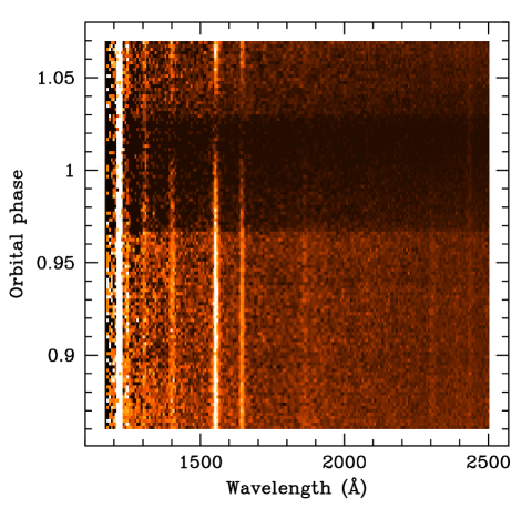
Figure 9: Trailed spectrum of UZ For, both observed orbits added and rebinned. The figure clearly shows the abrupt ingress and egress of the continuum source and the more gradual eclipse of the emission line source. It also shows a faint dip in the continuum and in the lines at $\Phi=0.90$ which occurs when the magnetically funneled section of the accretion stream crosses the line of sight to the white dwarf.

Figure 10: Extracted C iv light curves and best fits. Left: orbit 1, right: orbit 2. In each panel, ten light curves from different fit runs are overplotted (hard to recognize) to show the stability of the fit. The residuals are scaled down by a factor of 4 for clarity. The vertical dashed lines mark the ingress and egress of the white dwarf and, hence, approximately the begin of the ingress and egress of the magnetically funneled accretion stream.

5.3 Results

The light curves show small, but significant differences for the two orbits (Fig. 10). In orbit 1, the dip at $\Phi=0.9$ is slightly deeper than in orbit 2. However, this very small feature has only a marginal effect on the results. The dip is well known from X-Ray and EUV observations Warren et al. (1995) and has been observed to move in phase between $\Phi=0.88$ and $0.92$ on timescales of months Sirk and Howell (1998). The ingress of the accretion stream into eclipse is much smoother in orbit 1 than in orbit 2, where an intermediate brightness level around $\Phi=0.98$ with a flatter slope is seen. The C iv intensity maps resulting from our fits are shown in Fig. 11 for each observation interval separately. In Fig. 12, we show the relative intensity distributions of 10 fit runs for each orbit, proving that our algorithm finds the same result (except for noise) for each run. In Fig. 11, the resulting map from one arbitrary fit is shown.

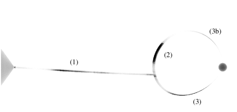
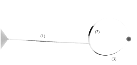
Figure 11: Resulting intensity maps of the accretion stream in UZ For. Left: Orbit 1, right: Orbit 2. Bright regions are printed in black, dark regions in white.

Figure 12: Resulting intensity distributions of the accretion stream in UZ For. Left: Orbit 1, right: Orbit 2. The results of 10 individual fit runs are overplotted in one graph to show the consistency of the fits. For an explanation of the plots see Fig. 4.

The brightness maps for the two orbits show common features and differences. Common in both reconstructed maps are the bright regions (1) on the ballistic stream, (2) on the dipole stream above the orbital plane, and (3) on the dipole stream below the orbital plane. In orbit 1, there is an additional bright region on the northern dipole stream which appears as a mirror image of region 3. We denominate it 3b. The difference between both maps is found in the presence/absence of region 3b, and in the different sharpness of region 1, which is much brighter and more peaked in orbit 1 than in orbit 2.

Remarkable is that we do not find a bright region at the coupling region $SR$, where one would expect dissipative heating when the matter rams into the magnetic field and is decelerated. We will comment on this result in Sect. 6.2.

The sharp upper border of region 2 has to be discussed separately: As one can see from the data, the flux of the C iv $\lambda$ 1550 emission ceases completely in the phase interval $\Phi\approx 0.01\dots 0.03$. Hence, all parts of the accretion stream which are not eclipsed during this phase interval can not emit light in C iv $\lambda$ 1550. For the assumed geometry of UZ For, parts of the northern dipole stream remain visible throughout the eclipse. Thus, the sharp limitation of region 2 marks the border between those surface elements which are always visible and those which dissappear behind the secondary star. Uncertainties in the geometry could affect the location of the northern boundary of region 2, but should not change the general result, namely that there is emission above the orbital plane that accounts for a large part of the total stream emission in C iv $\lambda$ 1550.

Region 3b has to be understood as an artifact: During orbit 1, the observed flux level at maximum emission line eclipse ($\Phi=0.01\dots 0.03$) does not drop to zero. Hence, our algorithm places intensity on the surface elements of the accretion stream which are still visible at that phase. Apparently, the evolution strategy tends to place these residual emission not uniformly on all the visible surface elements but on those closer to the WD, which leads to an intensity pattern that resembles the more intense region on the southern side of the dipole stream.

Figure 13: Intensity map of the accretion stream for orbit 1. The light curve used to generate this map was changed from the observed so that for each phase point the flux was randomly modified with a gaussian with $\sigma$ as described in Sect. 4.2. Compare with Fig. 11 and see text.

To underpin the fact that regions 1, 2, and 3 in our map are real features and not just regions which result by random fluctuations in the data, we test what happens to the reconstruction if the input light curve is changend. For the calculation which results in the map shown in Fig. 13, we generated a modified light curve from the data for orbit 1. For each phase step, we modified the flux, so that $F^{\prime}(\Phi)=F(\Phi)+1/2\cdot\sigma(\Phi)\cdot G$ is the new value. $\sigma(\Phi)$ is the local standard deviation as defined in Sect. 4.2, $G$ are gaussian-distributed random values. Since the map from the light curve $F^{\prime}(\Phi)$ does not show significant differences from the map corresponding to the original data $F(\Phi)$ (Fig. 11), we conclude that the features 1, 2, and 3 are real.

6 Discussion

We have, for the first time, mapped the accretion stream in a polar in the light of a high-excitation ultraviolet line with a complete 3d model of an optically thick stream. We have found three different bright regions on the stream, but no strong emission at the stagnation point of the ballistic stream. In the following we will discuss the physical processes which may lead to an emission structure like the one observed.

6.1 Emission of the ballistic stream

As mentioned in Sect. 2, single-particle trajectories with different inital directions diverge after the injection at $L_{1}$, but converge again at a point approximately one third of the way between $L_{1}$ and the stagnation region. This is where we find emission in the line of C iv $\lambda$ 1550. Possibly the kinetic properties of the stream lead to a compression of the accreted matter, resulting in localized heating. After the convergence point, the single-particle trajectories diverge slowly and follow a nearly straight path without any further stricture. Hydrodynamical modelling of the ballistic part of the stream is required to substantiate this hypothesis.

6.2 Absence of emission at the stagnation point

In the classical model of polars, it is assumed that the ballistically infalling matter couples onto the magnetic field in the stagnation region with associated dissipation of kinetic energy (e.g. Hameury et al., 1986). Thus, one would expect a bright region near $SR$. The absence of C iv $\lambda$ 1550 emision in the stagnation region could be due to the fact that there is no strong heating in the coupling region. Dissipation near $SR$ can be avoided if the material is continously stripped from the ballistic stream and couples softly onto the field lines, as proposed by Heerlein et al. Heerlein et al. (1999) for HU Aquarii.

Another possibility is that the matter is decelerated near $SR$, resulting in an increase in the density. This may result in an increase of the continuum optical depth, and, therefore, in a decrease of the C iv $\lambda$ 1550 equivalent width.

6.3 Emission of the dipole stream

On the dipole section of the stream, we find two generally different emission regions: The bright and small region above the stagnation point and the broader regions near the accretion poles of the white dwarf.

Near the accretion spots: On the magnetically funneled stream, we find one region of line emission (3) which we assume to be due to photoionization by high-energy radiation from the accretion spot. The mirror region 3b is an artifact which is created by the mapping algorithm to account for the non-zero flux level in orbit 1 in the phase interval $\Phi=0.01\dots 0.03$ (see Sect. 5.3). Even though the distribution of C iv emission on the accretion stream does not reflect the irradiation pattern in a straigthforward way, the presence of C iv emission at a certain location of the stream requires that this point is irradiated, if there is no other mechanism creating C iv line emission. In Fig. 14, we define the angles $\alpha_{1}$ and $\alpha_{2}$ and the distances $r$ and $R$. Assuming a point-like emission region at the accretion spot, the absorbed energy flux per unit area caused by illumiation from the accretion regions varies as $\cos\alpha_{1}\sin\alpha_{2}R^{3/2}/{r^{2}}$.

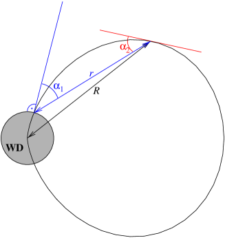
Figure 14: Dipole field line configuration. See Sect. 6.3.

The structure of this equation shows that the illumination of the accretion stream is at maximum somewhere between the accretion region and the point with $\alpha_{1}=0$. This corresponds to the brightness distribution which we derive from the data.

We suggest the following interpretation of the emission region above the stagnation point: Independent of whether the C iv emission in this region is due to photoionozation or collisional excitation, a higher density than in other sections of the stream is required. Matter which couples in $SR$ onto the field lines has enough kinetic energy to initially rise northward from the orbital plane against the gravitational potential of the white dwarf. If the kinetic energy is not sufficient to overcome the potential summit on the field line, the matter will stagnate and eventually fall back towards the orbital plane, where it collides with further material flowing up. This may lead to shock heating with subsequent emission of C iv $\lambda$ 1550. Alternatively, the photoinization of the region of increased density may suffice to create the emission peak. Yet another possibility is that the matter is heated by cyclotron radiation from the accretion column which emerges preferentially in direction perpendicular to the field direction. Crude estimates show, however, that the energy of the cyclotron emission does not suffice to produce such a prominent feature as observed. A detailed understanding of the emission processes in the accretion stream involves a high level of magnetohydrodynamical simulations and radiation transfer calculations, which is, clearly, beyond the scope of this paper.

6.4 Conclusion

We have successfully applied our new 3d eclipse mapping method to UZ Fornacis. In subsequent research we will allow additional degrees of freedom in the mapping process, using data sets with higher S/N and covering a larger phase interval.

Our attempts to image the accretion stream in polars should help in understanding the physical conditions in the stream, such as density and temperature. By comparison to hydrodynamical stream simulations, we will take a step towards the complete understanding of accretion physics in polars.